The Effect of Variable Air–Fuel Ratio on Thermal NOx Emissions and Numerical Flow Stability in Rotary Kilns Using Non-Premixed Combustion

Abstract

One of the quickest ways to influence both the wall temperature and thermal NOx emissions in rotary kilns is to change the air–fuel ratio (AFR). The normalized counterpart of the AFR, the equivalence ratio, is usually associated with premixed flames and studies of its influence on diffusion flames are inconsistent, depending on the application. In this paper, the influence of the AFR is investigated numerically for rotary kilns by conducting steady-state simulations. We first conduct three-dimensional simulations where we encounter statistically unstable flow at high inflow conditions, which may be caused by vortex stretching. As vortex stretching vanishes in two-dimensional flow, the 2D simulations no longer encounter convergence problems. The impact of this simplification is shown to be acceptable for the thermal behaviour. It is shown that both the wall temperature and thermal NOx emissions peak at the fuel-rich and fuel-lean side of the stoichiometric AFR, respectively. If the AFR continues to increase, the wall temperature decreases significantly and thermal NOx emissions drop dramatically. The NOx validation, however, shows different results and indicates that the simulation model is simplified too much, as the measured NOx formation peaks at significantly fuel-lean conditions.

1. Introduction

Rotary kilns are long cylindrical furnaces that are horizontally positioned and slightly inclined. A wide range of material processing industries make use of these devices, such as cement production, metallurgy, and waste treatment [1]. Due to the inclination and axially rotating motion of the kiln, the raw-material gradually moves from the cold (upper) end towards the hot (lower) end, where the burner is located. A schematic is shown in Figure 1). The primary role of these devices is to gradually heat the material. We study its application in the cement industry where the material bed is mixed, heated and subjected to sintering reactions to form clinker. The material leaves the furnace at the lower end to be further processed. Sufficiently high temperatures are required to heat the material to reach the sintering reactions, with flame temperatures exceeding 2000 K. This makes the process prone to the formation of thermal nitric-oxides (thermal NO or thermal NOx).

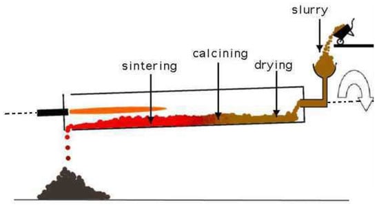
Figure 1. Schematic of the rotary kiln [2]. Reproduced with permission from WHD Microanalysis Consultants Ltd.

With the ever-increasing environmental impact and growing demand in cement production, improvement of kiln efficiency and mitigation of pollutant formation have been the central concern of cement manufacturing technology. As in-situ experimental campaigns are hampered by high temperatures and harsh operating conditions, numerical simulation is the prominent alternative for gaining insight and finding optimal solutions for this cause. Both techniques were studied extensively on rotary kilns in [3].

Computational Fluid Dynamics (CFD) packages have been used to study different aspects of the rotary kiln. E.g., in [4] we see how CFD can aid in the operation and design of a kiln to meet the specified requirements. We extended this model in [5] by adding the refractory lining, to allow the wall temperature to develop more realistically. Some other recent CFD studies related to rotary kilns include the modeling of the aerodynamics [6], combustion [7,8,9,10], multiphase flow [11], coupling with 1D material bed model [12], heat transfer coupled with DEM for granular flow [13,14], and combinations hereof [15,16]. Depending on the targets, essentially the more physics that are involved, the less advanced mathematical models are used due to lack of computational resources.

Our aim is to reduce the thermal NO emissions of an actually operating kiln burning on natural gas. As shown in our latest work [17], changing the air inlet geometry shows promising results in reducing both the peak temperatures as well as thermal NOx emissions. However it does require rebuilding the inlet side of the kiln and reinstalling the combustion air infrastructure. An easier solution would be to modify the operating condition, which is a matter of turning the valves. It was shown in [18] that increasing the volumetric air–fuel ratio (AFR) leads to both lower flame temperature and wall temperature, thus preventing ring formation. The lower flame temperature indicates that thermal NOx formation may also drop, though it is not that simple because more oxygen and nitrogen is provided as well.

The normalized version of the AFR, the fuel-air equivalence ratio is generally associated with premixed flames which has the widely known parabolic relation with the adiabatic flame temperature where the maximum temperature occurs slightly on the fuel-lean side of the stoichiometric equivalence ratio (>1). As for diffusion flames, such as in rotary kilns, the reactions take place in the flame front where the fuel and oxidiser occur in stoichiometric ratio’s, leading to maximum adiabatic temperature, regardless of the equivalence ratio [19]. Which is why the mixture fraction is a better suited parameter for diffusion flames in general. The AFR however is something that the operator can control, unlike the mixture fraction. However, unlike premixed flames, it is less obvious for diffusion flames whether NOx emissions will increase or decrease with the AFR, and depends on the type of diffusion flame application, as is recently shown in [20]. Another study is done in [21] on confined diffusion flames, where it is shown that depending on the confinement ratio, the AFR either has a small or large impact on NOx emissions. However, the range of the AFR is small and is on the fuel-rich side, while we aim for the fuel-lean side.

There are some studies applied to rotary kilns where, partially, the influence of the AFR on NOx formation is investigated. In [22], both experimental and numerical works (using a chemical reactor model) are done on a small pilot scale and full scale kiln. In [23] experimental work is conducted on the precalciner whereas the kiln is experimentally simulated. In both mentioned studies, the NOx formation increases with the AFR on the lean side (excess air). This has to do with the fact that they are using coal as energy source, which contains a large amount of fuel-bound nitrogen, leading to fuel NOx formation to dominate with higher excess air.

No CFD related study has been done thus far on the effect of the AFR on thermal NOx emissions in rotary kilns using natural gas as fuel. Therefore, the focus of our work is to find out how the temperatures and thermal NOx emissions are affected by the AFR, as this is a relatively simple way to influence both outcomes. This is investigated numerically, and experimentally in this paper. The required physics are integrated in a solver for which we make use of the library of the CFD toolbox OpenFOAM. We use the developed code multiRegionReactingFoam [24,25]. This solver couples the conjugate heat transfer (CHT) utility of OpenFOAM with the combustion utility. Additionally, the Eddy Dissipation Model is implemented for the turbulence-chemistry interaction, and for the external heat loss we implement the Robin boundary condition.

The paper is structured as follows. We first explain the mathematical models to solve the required physics in Section 2. We then carry out three-dimensional simulations in Section 3, followed by a discussion in Section 4. Afterwards we conduct two-dimensional simulations in Section 5 and present the results. We draw conclusions in Section 6.

2. Governing Equations and Mathematical Model

For this work we conduct RANS simulations. Therefore in the fluid domain, we solve the Favre-averaged transport equations of mass, momentum, chemical species and sensible enthalpy [19]. These are respectively described by the following equations

$$\frac{\partial \left(\overline{\rho }\right)}{\partial t}+\nabla ·\left(\overline{\rho }\tilde{u}\right)=0,$$

(1)

$$\frac{\partial \left(\overline{\rho }\tilde{u}\right)}{\partial t}+\nabla ·\left(\overline{\rho }\tilde{u}\tilde{u}\right)=-\nabla \overline{p}+\nabla ·\mu \nabla \tilde{u}-\nabla ·\overline{\rho }\widetilde{u″u″},$$

(2)

$$\frac{\partial \left(\overline{\rho }\widetilde{Y_{\alpha }}\right)}{\partial t}+\nabla ·\left(\overline{\rho }\tilde{u}\widetilde{Y_{\alpha }}\right)=\nabla ·\overline{\rho }\mathsf{\Gamma }\nabla \widetilde{Y_{\alpha }}-\nabla ·\overline{\rho }\widetilde{Y_{\alpha }″u″}+{\tilde{R}}_{\alpha },$$

(3)

$$\frac{\partial \left(\overline{\rho }\tilde{h}\right)}{\partial t}+\nabla ·\left(\overline{\rho }\tilde{u}\tilde{h}\right)=\frac{D}{Dt}\overline{p}+\nabla ·\frac{\lambda }{c_p}\nabla \tilde{h}-\nabla ·\overline{\rho }\widetilde{h″u″}+{\tilde{Q}}_c+{\tilde{Q}}_r,$$

(4)

where u is the velocity, $\rho$ is the density, p is the pressure, $\mu$ is the laminar dynamic viscosity, $Y_{\alpha }$ is the species mass fraction of species $\alpha$, $\mathsf{\Gamma }$ is the species diffusion coefficient, R is the reaction rate of species $\alpha$, h is the specific sensible enthalpy, $c_p$ is the specific heat capacity at constant pressure and $\lambda$ is the thermal conductivity. The heat source terms $Q_c$ and $Q_r$ are due to combustion and thermal radiation, respectively. The over-bar and tilde notations denote the average values, while the double quotation marks stand for the fluctuating components due to turbulence. Several source terms are neglected, such as body forces and viscous heating.

The refractory lining is considered a solid region for which we model its energy transfer by solving the equation of enthalpy for solids

$$\frac{\partial \left(\overline{\rho }h\right)}{\partial t}=\nabla ·(\lambda \nabla T).$$

(5)

While Equation (5) is solved separately from Equations (1)–(4), the thermal energy transport between the fluid and solid domains are coupled after each iteration by applying the following domain interface conditions, to ensure continuity of both the temperature and heat flux [26]:

$$T_{f,int}=T_{s,int}$$

(6)

and

$${\lambda }_f\frac{\partial T_f}{\partial y}{|}_{int,y=+0}={\lambda }_s\frac{\partial T_s}{\partial y}{|}_{int,y=-0}.$$

(7)

The subscripts f, s and $int$ respectively stand for fluid, solid and interface. y is the local coordinate normal to the solid. Unknown terms appear on the right-hand side of the transport equations of the fluid domain due to Favre averaging that have to be closed. These will be treated in this section, followed by the elaboration of the heat transfer at the interface.

2.1. Turbulence

The last term of Equation (2) represents the unknown Reynolds stresses. These are solved by employing the Boussinesq hypothesis, which is based on the assumption that in turbulent flows, the relation between the Reynolds stress and viscosity is similar to that of the stress tensor in laminar flows, but with increased (turbulent) viscosity:

$$-\nabla ·\overline{\rho }\widetilde{u_i^{\prime \prime }{u}_j^{\prime \prime }}={\mu }_t\left(\frac{\partial u_i}{\partial x_j}+\frac{\partial u_j}{\partial x_i}\right)-\frac{2}{3}\left(\rho k+{\mu }_t\frac{\partial u_k}{\partial x_k}\right){\delta }_{ij},$$

(8)

where ${\mu }_t$ is the turbulent dynamic viscosity and k the turbulent kinetic energy. The Reynolds stresses are closed with the Realizable k-$ϵ$ turbulence model [27], which solves two additional transport equations: One for the turbulent kinetic energy k, and the other for its dissipation rate $ϵ$

$$\begin{array}{cc}\hfill \frac{\partial \left(\overline{\rho }k\right)}{\partial t}+\nabla ·\left(\overline{\rho }\tilde{u}k\right)& =\nabla ·\left[\left(\mu +\frac{{\mu }_t}{{\theta }_k}\right)\nabla k\right]+{\mu }_t{\left(\frac{\partial u_i}{\partial x_j}\right)}^2-\overline{\rho }ϵ,\hfill \end{array}$$

(9)

$$\begin{array}{cc}\hfill \frac{\partial \left(\overline{\rho }ϵ\right)}{\partial t}+\nabla ·\left(\overline{\rho }\tilde{u}ϵ\right)& =\nabla ·\left[\left(\mu +\frac{{\mu }_t}{{\theta }_{ϵ}}\right)\nabla ϵ\right]+\overline{\rho }{c}_{1}Sϵ-\overline{\rho }{c}_2\frac{{ϵ}^2}{k+\sqrt{\nu ϵ}},\hfill \end{array}$$

(10)

where S is the modulus of the mean strain rate tensor and $c_1$ is a function of k, $ϵ$ and S. ${\theta }_k$, ${\theta }_{ϵ}$ and $c_2$ are constants. The effect of buoyancy is neglected as well as other source terms.

2.2. Combustion

We implement the Eddy Dissipation Model (EDM) [28] in the OpenFOAM library, in order to calculate the mean chemical source term ${\tilde{R}}_{\alpha }$. This implies that only the 1-step methane reaction mechanism is used. The EDM is an attractive model to use due to its computational efficiency and reasonable accuracy. The rate of reaction is taken as the minimum of the three rates for fuel, oxidant and products

$${\tilde{R}}_{\alpha }=-A\overline{\rho }\frac{ϵ}{k}min\left({\overline{Y}}_F,\frac{{\overline{Y}}_O}{\nu },B\frac{{\overline{Y}}_P}{1+\nu }\right),$$

(11)

where A and B are user defined model constants that by default are respectively equal to 4 and 0.5, and $\nu$ is the stoichiometric coefficient. As the EDM is a ‘mixed is burnt’ model type, it excludes the effects of chemical kinetics and is derived from the aspects of combustion occurring at high Damköhler and Reynolds numbers where reactions are limited by turbulent mixing [19]. Therefore, the underlying assumption for choosing this model is that in rotary kilns the combustion is indeed mainly controlled by turbulent mixing. The model is validated in [29] where it is shown that the flame temperatures are over-predicted, as can be expected from 1-step reaction mechanisms with infinitely fast reaction rates. However, the profiles are well captured. When thermal radiation is included, the over predictions can be reduced.

The heat release due to combustion $\widetilde{Q_c}$ follows from the calculations of ${\tilde{R}}_{\alpha }$

$$\widetilde{Q_c}=-\sum _{\alpha =1}^{N-1}\Delta h_{f,\alpha }^o\widetilde{R_{\alpha }},$$

(12)

where $\Delta h_{f,\alpha }^o$ is the formation enthalpy of species $\alpha$, and N is the total number of species, of which only nitrogen is considered chemically inert by the EDM.

2.3. Thermal Radiation

The mean radiation source term $\widetilde{Q_r}$ for the enthalpy transport equation is obtained by employing the P1 approximation which solves the following equation for a non-scattering medium

$$-\nabla ·\left(\frac{1}{3\kappa }\nabla G\right)=\kappa (4\sigma T^4-G),$$

(13)

where G is the total incident radiation, $\sigma$ is the Stefan–Boltzmann constant and $\kappa$ is the absorption coefficient of the medium. The radiation source term appears on the LHS of the equation. The P1 approximation is subject to the following Robin boundary condition [30]

$$-\frac{1}{3\kappa }\mathbf{n}·\nabla G=-\frac{{\kappa }_w}{2(2-{\kappa }_w)}(4\sigma T_w^4-G_w).$$

(14)

To solve Equation (13), the local absorption coefficient of the gas mixture $\kappa$ has to be determined. This is a function of gas composition, temperature, wavelength, and pressure. Within the radiation spectrum, the individual species absorb and emit through thousands of wavelengths, which makes it too expensive to calculate all of them. While models exist that average the amount of the wavelength lines up to a handful of broad bands (Wide Band Model), we choose to apply the grey gas assumption where the absorption coefficient is an average over the whole spectrum. While this is a simplification, the model still accounts for the gas composition, temperature and pressure. The wall has a constant absorption coefficient (${\kappa }_w$) of 0.6. Adding radiation to the problem alters the interface condition (Equation (7)) to

$${\lambda }_{eff}\frac{\partial T_f}{\partial y}{|}_{int,y=+0}+q_{r,in}-q_{r,out}={\lambda }_s\frac{\partial T_s}{\partial y}{|}_{int,y=-0},$$

(15)

where $q_{r,in}$ is the incident radiative heat flux absorbed by the solid and $q_{r,out}$ is the reflected and emitted radiative heat flux leaving the solid.

2.4. External Heat Loss

In order to have a more realistic thermal boundary condition at the outer wall surface, we incorporate the environmental heat loss by setting a Robin boundary condition on the outer wall surface. For this, we assume that there is no wind, hence no forced convection, although this can be incorporated as well by means of the convective heat transfer coefficient. We calculate the radiative heat loss as follows.

Referring to Figure 2, the inner wall temperature at $y=$ 0 is known and defined as $T_{w,is}$.

$${T|}_{y=0}=T_{w,is}.$$

(16)

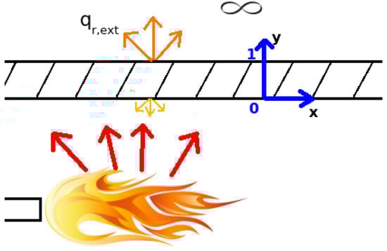
Figure 2. Schematic of a confined turbulent flame with radiative heat loss to the environment via the wall.

At the outer wall surface (y = 1) we use the Stefan-Boltzmann law to determine the flux, so that

$${\lambda }_s\frac{\partial T}{\partial y}{|}_{y=1}=q_{r,ext}=ϵ\sigma (T_{w,os}^4-T_{\infty }^4),$$

(17)

where $T_{\infty }$ is the ambient temperature which is set to 288,15 K. Using Equations (16) and (17), it can be derived that the outer wall surface temperature

$$T_{w,os}=\frac{ϵ\sigma }{{\lambda }_s}(T_{w,os}^4-T_{\infty }^4)y_1+T_{w,is},$$

(18)

where $y_1$ is equal to the thickness of the refractory wall.

2.5. Thermal NOx

The thermal NOx (or NO) concentration is computed using the extended Zel’dovich mechanism in the post-processing stage (see, e.g., Section 12.28 in [31] and Section 17.1 in [32]). We make use of the implementation of this post-processor in OpenFoam realized by Kadar [33]. The mass fractions of the species O and OH are obtained using the partial equilibrium assumption.

3. Three-Dimensional Flow Simulations

3.1. Set-Up

The combustion in the cement kiln that we consider is fed by a non-premixed turbulent flow and with methane as fuel. We like to study the effect of varying air–fuel ratio (AFR) by volume, which is defined as ratio of the volumetric flow rates of air to fuel.

For this, we continue our work in [17] by keeping the mass flow rates of the fuel inlets and primary air inlet constant and increasing the secondary air inlet mass flow rate further (see Figure 3).

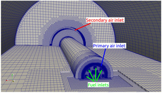
Figure 3. Mesh inside of the kiln with a modified (annular) secondary air inlet. The figures show the multi-nozzle burner and cooling slot in the foreground, the burner pipe and the secondary air inlet channel in the background. Only the lower half of the kiln’s internal volume grid is visible (some unclipped cells appear out of the plane) to show the refinement regions. For increased visibility, a coarse mesh is shown here. Ref. [17] Reproduced with permission from [Domenico Lahaye, Mohamed el Abbassi, Kees Vuik, Marco Talice and Franjo Juretić], [Fluids]; published by [MDPI], [2020].

Some important simplifications are applied to the simulations. As the inclination angle and kiln’s rotational speed are very low, they are excluded. Due to complexity of implementing a model for the sintering reactions of the material bed, this is excluded as well. As the material bed only accounts for 5% of the total kiln’s volume, with a residence time of 30 min or more, it will have limited impact on the reactive flow.

Hexahedral dominant cartesian meshes are generated for the kiln geometries using cfMesh [34], consisting of 4.2 million to 4.4 million cells depending on the secondary air inlet geometry. The reacting flow and conjugate heat transfer simulations are performed with the OpenFOAM-v5.0 solver multiRegionReactingFoam [25]. The thermal NOx post-processor is taken from [33].

3.2. Aerodynamics

As a first analysis, the reactive flow simulation is shown here and compared with the results in [18], where the mixture has an AFR of 9. This is the actually operating kiln and its geometry is referred to as geometry A, which has a rectangular air inlet on top of the burner attachment.

To understand the results of temperature and emissions better we investigate the stream pattern first in Figure 4, which qualitatively agrees well with [18]. The pattern can be decomposed into four streams.

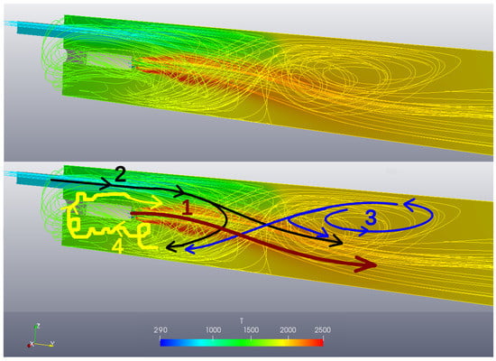
Figure 4. Stream pattern and temperature contour plot of the kiln geometry A.

• Stream 1: The high momentum primary jet leaving the burner.
• Stream 2: The secondary co-flow stream entering from the rectangular inlet at a much lower velocity.
• Stream 3: Upper recirculation zone due to Craya-Curtet flow.
• Stream 4: Lower recirculation zone due to backward facing step.

We observe that all four streams interact with each other. The interactions of streams 1, 2 and 3 are similar as in a Craya-Curtet flow. Stream 2 slows down due to the adverse pressure gradient downstream and is being sucked towards the high momentum stream 1 where the static pressure is lower, causing stream 2 to detach from the wall. When stream 2 bends downwards it separates into two directions. Part of the stream is entrained by stream 1, flowing towards the kiln outlet, while the other part turns upstream towards stream 4. Stream 4 is a recirculation zone that exists due to the geometry of the kiln, which is similar to a backward facing step. The recirculation zone in stream 3 results from the detachment of stream 2, and causes stream 1 to bend downwards. The flow of stream 3 that escapes the recirculation zone is either entrained by stream 1, or by stream 2 towards stream 4. In order to reach stream 4 however, it has to go around stream 1. The recirculation zone of stream 4 is very unstable. The reason for this is that the flow coming from streams 2 and 3, and from the vortex itself, are severely disturbed when flowing around the burner jet of stream 1.

3.3. Flow Instability at High Reynolds Number

The AFR is increased by increasing the secondary air inlet mass flow rate. While we get a steady state solution at AFR of 9, this only lasts until we increase the AFR to 10. Beyond the AFR of 10, the flow becomes unstable and the solution procedure is not converging. On the other hand if we reduce the AFR to values lower than 9, the flow remains stable and the solution procedure converges sooner.

Figure 5 shows the stream pattern on the vertical cross-section for several geometries and for a range of AFR’s. In the left column we see the stream pattern for the real kiln geometry (geometry A). We see that the upper recirculation zone is pushed further downstream by the increasing momentum of the secondary air inlet that increases with the AFR. Beyond AFR of 10 this vortex breaks and the flow becomes unstable for which no steady-state solution can be found. The instability beyond AFR of 10 has shown to be a problem, as we are interested in higher ratio’s as well.

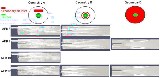
Figure 5. Stream patterns at different air–fuel ratio’s for the original kiln (geometry A), the modified kiln with annular air inlet (geometry B) and the modified kiln with co-flow air inlet over the entire lateral cross-section around the burner (geometry D).

To solve this issue we use a modified air inlet geometry in order to have a stable, axisymmetric and predictable flow (geometry B). With an annular inlet we expect that the concentric recirculation zone will remain stable with higher AFR’s as well, since there is no collision between jets and vortices. Surprisingly, the flow becomes unstable as well at AFR’s beyond 9 and without convergence of the simulation. Even at AFR of 9, the simulation took much longer to converge compared to the original geometry. Observing the stream pattern snap shots in Figure 5 (2nd column), the dynamic and asymmetric behaviour of the recirculation zone can be seen at increasing AFR. We see a varying elongation and shortening of the recirculation zone. The number of vortices that the recirculation zone consist of, alternates between one and two during the shortening and elongation respectively.

4. Understanding the Purpose of RANS and the Meaning of Stability

For both the original and modified geometry (A and B), we see a trend that increasing the Reynolds number (which is proportional with AFR), the more instability occurs. This of course makes sense as the flow is getting more and more turbulent and the dampening of the viscous forces gets smaller. For pipe flows, the flow is completely turbulent at Reynolds numbers $R{e}_D$ above 4000. $R{e}_D$ in the kiln is about 30,000, which is considered highly turbulent.

What is meant with unstable flow when turbulent flow is inherently unstable? If $R{e}_D$ is below 4000, the flow is laminar which is truly stable in the sense that the flow does not change in time and therefore a steady-state solution exists. When the laminar flow is disturbed, by any reason, it will ‘stumble’ and a chain reaction of flow eddies is caused which becomes chaotic, leading to turbulent flow. The flow is now changing over time, and a steady-state solution does not exist. The Reynolds number tells us that the higher its value becomes, the sooner the laminar flow will transition to turbulent flow and the larger the spectrum of length scales of the eddies one has to solve in time.

The RANS method is a mathematical method to obtain the steady-state property of laminar flow back because it saves much time. What it physically does is it makes the flow more viscous in order to dampen the turbulent fluctuations, so that the flow will look laminar again, or statistically stationary. This is done by adding the turbulent viscosity ${\mu }_t$ to the laminar viscosity in the momentum equation. This method is justified by the fact that the time-average of turbulent flow also looks laminar. However the dampening effect of making the flow more viscous has a limit. At a certain point, or to be more precise, certain high enough Reynolds number, the sensitivity to disturbances becomes so large that even the ‘thickened’ turbulent flow becomes unstable again. Or as we can call it, statistically unstable.

This trend that we see with flow instability and Reynolds number helps us to understand the results better. We see that compared to non-reacting flow, stability and convergence improves with reacting flow because the average Reynolds number, e.g., at AFR of 9, drops from 29,750 to 21,006. The stability and convergence also improves by simplifying the geometry even more so that less disturbances occur, while keeping the average Reynolds number the same. This can by seen in the stream pattern of geometry D in Figure 5 where the secondary air flows in from the entire diameter around the burner, which removes the recirculation zone cause by the annular air inlet (geometry B) and results in a pure Craya-Curtet flow. Geometry D does not suffer from convergence problems for the full range of AFR but due to lack of mixing, the temperatures are relatively low and not representative for geometry A.

Vortex Stretching

The question now is what causes the flow to be unstable in the geometry with the annular air inlet. We believe the answer lies when we plot the streamlines. In paraView we plot the streamlines through a line, so that the stream pattern will look like a sheet with several three-dimensional rotations. We always get a full three-dimensional flow as a result, with the complete concentric recirculation zone. Apparently the streamlines propagate in radial direction (‘out of the plane’) around the burner.

This gets even more clear when we plot the streamlines through a line at the center of the vortex. In Figure 6 we see how the streamlines propagate in radial direction in a swirling motion when we increase the maximum length of the streamlines. This phenomenon is known as vortex stretching, which is the key mechanism of the turbulent energy cascade and an essential aspect of turbulence [35]. We believe this causes the instability and explains why this problem does not occur in two-dimensional simulations. Vorticity is a fundamental property of turbulence and its evolution can be obtained by taking the curl of the Navier-Stokes equations [36], which for the case of incompressible flow leads to

$$\frac{D\left(\overline{\omega }\right)}{Dt}=(\overline{\omega }·\nabla )\overline{u}+\nu {\nabla }^2\overline{\omega }$$

(19)

where $\omega$ is the vorticity, which is the curl of the velocity, $\nabla \times \overline{u}=\overline{\omega }$. Equation (19) is known as the vorticity equation where angular momentum is conserved. The first term on the right hand side of Equation (19) represents vortex stretching. Mathematically it can be derived that this term vanishes for two-dimensional flow (see e.g., [37], Section 1.3) and explains why vortex stretching is purely a three-dimensional phenomenon.

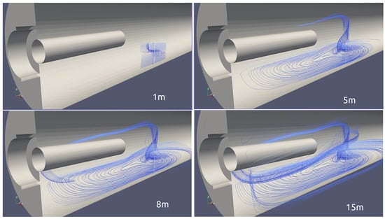
Figure 6. Development of the vortex stretching with increasing streamline length.

What we learn from this is that symmetric geometries with symmetric boundary conditions may still lead to asymmetric flows with steady RANS simulations. This is also observed in [38] and therein referenced literature.

5. Two-Dimensional Axisymmetric Simulations

We have seen how vortex stretching leads to statistically unstable flow in three dimensions. This instability does not occur in 2D axisymmetric simulations. Therefore, in order to continue investigating the effect of increasing the AFR to higher values, we choose to conduct the simulations of this analysis in 2D and are aware of neglecting the effect of vortex stretching. For this, we have to modify Geometry B (with the annular shaped secondary air inlet) by making the fuel inlet axisymmetric as well. This results in Geometry C where the fuel inlet is also annular shaped (see Figure 7). The fuel inlet thickness is determined such that the high fuel inlet Mach number remains roughly the same as in geometries A and B. Geometry C is the exact 3D version of its 2D axisymmetric counterpart. The 2D mesh consists of 92.634 control volumes of which the solution is grid independent. The dimensions of the kiln and the wall is shown in Figure 8.

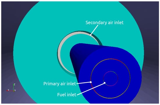
Figure 7. Modified kiln geometry C where all three inlets are annular shaped.

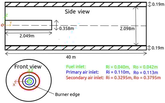
Figure 8. Dimensions (not to scale) of the modified kiln geometry C where all three inlets are annular shaped.

5.1. Boundary Conditions

For the sensitivity analysis of varying AFR we keep the mass flow rates of the fuel inlet and primary air inlet constant at 0.1 kg/s and 0.15 kg/s, respectively. The AFR is increased from 9 to 14 by raising the secondary air inlet flow. Further boundary conditions are shown in Table 1. The wall properties are given in Table 2.

Table 1. Boundary conditions for the kiln model C. zG stands for the Neumann boundary condition zeroGradient. Species are denoted in mass fractions.

Variable	Fuel Inlet	Primary Air	Secondary Air	Gas-Wall Interface	Outer Wall Surface
T[K]	293	293	773	Coupled	$q_{r,ext}$ *
$Y_{C{H}_4}$	1	0	0	zG	-
$Y_{O_2}$	0	0.23	0.23	zG	-
$Y_{N_2}$	0	0.77	0.77	zG	-

* external heat loss is included.

Table 2. Thermal properties of the refractory wall.

Density $\mathit{\rho }$	Thermal Conductivity ${\mathit{\lambda }}_{\mathit{s}}$	Specific Heat Capacity ${\mathit{c}}_{\mathit{p}}$	Emissivity ${\mathit{\kappa }}_{\mathit{s}}$
2800 kgm−3	$2.1$ Wm−1K−1	860 Jkg−1K−1	$0.6$ m−1

5.2. Effect on Wall Temperature

To verify the results in 2D, Figure 9 shows the streamline plot on the vertical longitudinal cross-section, coloured by the temperature contour. The flow is statistically stable with the familiar concentric recirculation zone as we expected. It is clear that the recirculation zone consist of two annular vortices that are connected to each other, where the most upstream vortex arises like in any confined jet flow and the downstream vortex is generated by the Craya-Curtet flow condition. While the flow stability is a major difference between the simulations in 2D and 3D, when we look at the wall temperature (see Figure 10) we see that the difference is very small. The temperature profile for the 2D is slightly shifted downstream by 2.5% of the kilns length.

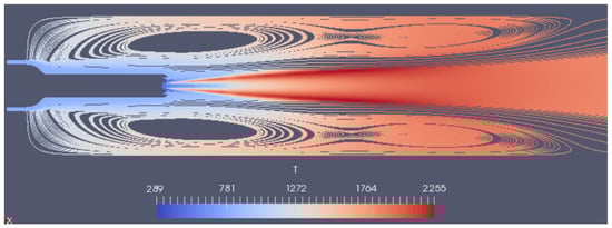
Figure 9. Streamline and temperature contour plot on the vertical longitudinal cross-section with the 2D simulation. For improved visibility, the upper half is mirrored.

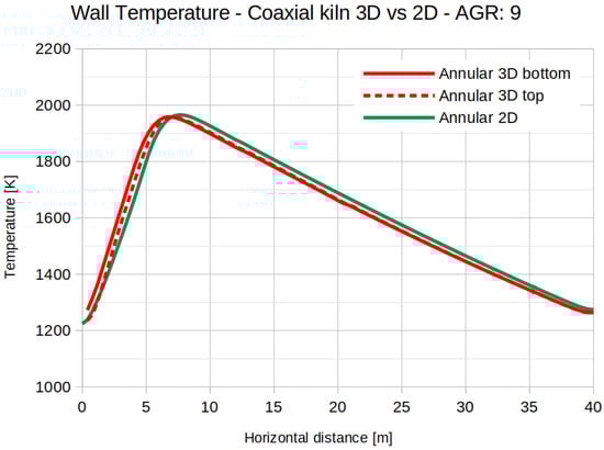
Figure 10. Computed top and bottom wall temperature along the axis of the kiln, 2D (green) vs. 3D (red). AFR: 9.

This difference in wall temperature is acceptable and allows us to continue investigating the effect of changing AFR on the wall temperature, which can be seen in Figure 11. As the AFR continues to increase, the wall temperature throughout the kiln drops. This makes sense. Surprisingly the wall temperature peaks at an AFR of 9 and not at the stoichiometric AFR of 9.5. We know that the wall is heated predominantly by the flame via thermal radiation which is related to the flame temperature. Figure 12 shows that the maximum flame temperature indeed peaks at the fuel-rich side of stoichiometric AFR. Theoretically the adiabatic flame temperature peaks at stoichiometry. For diffusion flames (like in our case), this even occurs at all AFR as reaction always takes place at stoichiometric condition regardless of the global AFR [19]. However, in reality heat is lost due to dissociation of the products. Since the extent of dissociation is greater on the lean side, the peaking occurs on the rich side. Moreover, the reduced momentum of the co-flow at lower-than-stoichiometric AFR may also contribute in the increased temperature due to less heat dissipation by the secondary inlet stream.

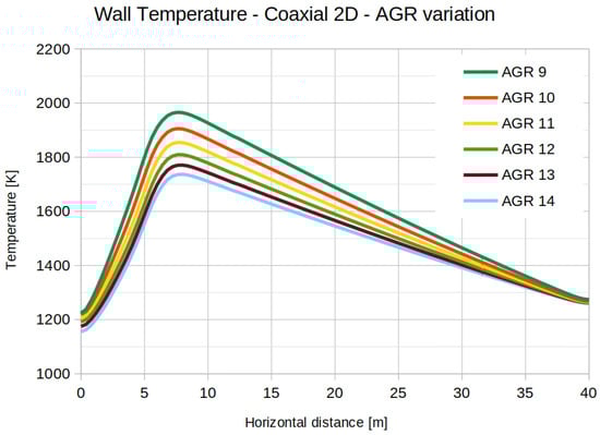
Figure 11. Computed wall temperature in the longitudinal direction of the kiln for different AFR’s.

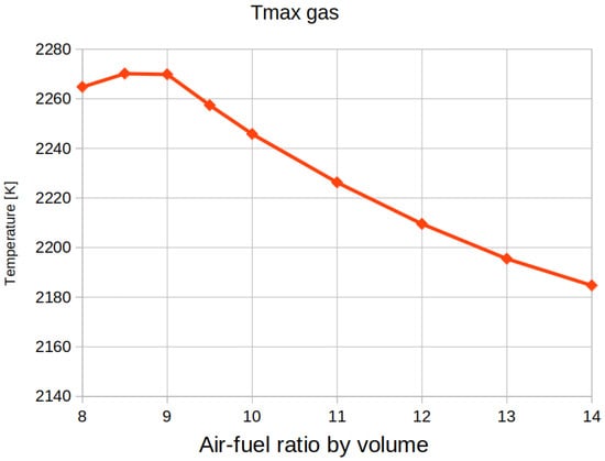
Figure 12. Computed maximum gas temperature for different AFR’s.

5.3. Effect on Thermal NOx Formation

Figure 13 shows the average concentration of thermal NOx at the outlet as a function of AFR. Contrary to the maximum flame temperature, thermal NOx formation relatively peaks on the lean side of stoichiometry due to competition of other species that react with oxygen as well. Figure 14 helps to understand the complexity of thermal NOx formation. Not only does it depend on the gas temperature and oxygen concentration, but on the flow as well, as was proven in [17]. An example in Figure 14 is that the temperature profile of AFR’s 8 and 10 are similar but the oxygen concentration is less in the hot region of the gas in the case for AFR of 8. Secondly, the thermal NOx contour plot shows that the NOx concentration peaks at an AFR of 9, but when we look at the outlet (Figure 13) more thermal NOx is emitted at an AFR of 9.5. The streamlines show that more NOx is trapped in the vortex for the AFR of 9, which explains why less NOx is emitted at the outlet.

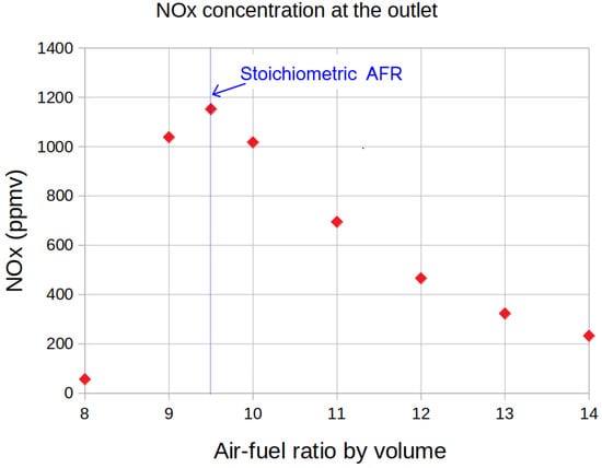
Figure 13. Average thermal NOx concentration at the outlet of the kiln for different AFR’s.

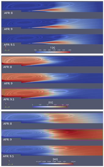
Figure 14. Contour plot of the temperature, and the mass fractions of oxygen and thermal NOx respectively for three different air–fuel ratio’s from fuel-rich mixture (AFR 8) to stoichiometric mixture (AFR 9.5). The minimum temperature is deliberately set at 1900 K to highlight the critical areas where thermal NOx can potentially be formed.

5.4. Preliminary NOx Validation

As a first attempt to validate the varying AFR simulations, the NOx concentration at the outlet of geometry C is compared to measurements of the actually operating kiln with geometry A. The box plot of the measurements is shown in Figure 15, where the simulation data are added. Recall that the simulation model is simplified, which makes it not a really fair comparison. Not only are the geometries different but the model is also without rotation, inclination and material bed flow. On the other hand, the material bed has a cooling effect on the refractory wall, and therefore the measurements can only be conducted during operation, i.e., with flowing raw material. Moreover, the detector does not distinguish between thermal NOx and other sources of NOx, while the model predicts thermal NOx exclusively.

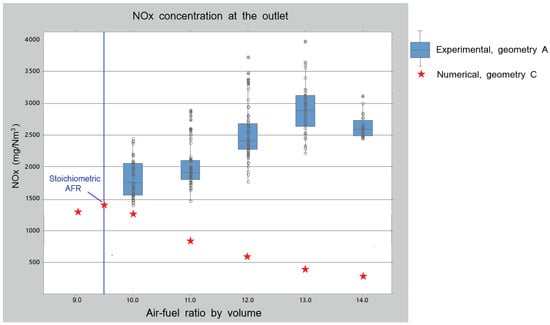
Figure 15. Average thermal NOx concentration at the outlet of the kiln for different AFR’s.

Other than that, we can say that there are similarities as well. The predicted and measured concentrations are within an order of magnitude, and both show a peak. The aerodynamics has a major influence on the thermal NOx formation and this drops significantly when changing the rectangular air inlet of geometry A to an annular inlet as in geometry C. It therefore makes sense that the simulations in Figure 15 predict less NOx. Surprisingly, the measured data show a peak far beyond stoichiometry, around the AFR of 13. This is counter-intuitive, as the theory suggests that the maximum should lie around the stoichiometric AFR. While studies, such as in [20], have shown that for diffusion flames it may increase with leaner mixtures (constant adiabatic temperature and more oxygen available). Moreover, since the actually operating kiln is burning natural gas which contains nitrogen, fuel NOx may form with excess air, as what occurs with coal combustion shown in [22,23]. However, we are aware that many factors play a role that leads to this behaviour that we see in the measurements. One thing is certain, which is that the simulation model needs to be made more complex in order to get closer to understand where the large shift of the peak comes from.

6. Conclusions and Recommendations

The objective of this paper is to show how varying AFR’s with non-premixed combustion affects the thermal process and thermal NOx emissions in rotary kilns as this was not clear from the literature.

• In this paper we discuss the numerical flow stability of our simulations. Three-dimensional simulations have shown that we are limited in carrying out steady state simulations at low AFR’s only. Even when the geometry and boundary conditions are symmetric, at high enough AFR’s the flow becomes statistically unstable and convergence becomes unfeasible. One of the causes is due to vortex stretching which highly influences the flow at high enough Reynolds number. Therefore symmetric geometries with symmetric boundary conditions may still lead to asymmetric flows with steady RANS simulations.
• To capture the varying effects of the vortices, it is recommended to carry out transient simulations. However, it will lead to much longer run times, even with URANS. This is mainly due to the shear size of the kiln with about 30 s residence time of the flow, while the CFL-condition (<0.2) requires that the time steps should be of the order 1 × ${10}^{-9}$ s or less, due to the limitation of the fuel inlets where the inlet speed reaches Mach 0.8 and the cell size is less than one mm.
• Two-dimensional simulations have shown to be successful as the phenomenon of vortex stretching vanishes and high AFR’s no longer lead to convergence problems. The impact of this simplification is shown to be acceptable for the thermal behaviour.
• It is shown that both the wall temperature and thermal NOx emissions peak at fuel-rich and fuel-lean side of the stoichiometric AFR, respectively. If the AFR continues to increase, the wall temperature decreases significantly and thermal NOx emissions drop dramatically. This is in accordance with the theory.
• The NOx validation however has shown unexpected results and indicates that the simulation model is simplified too much as the measured NOx formation peaks at significantly fuel-lean conditions. It is therefore recommended to include kiln rotation and inclination, detailed reaction mechanism (including other NOx species) and, as a last optional resource, a model for the material bed reactions and heat transfer.

References

- Boateng, A. Rotary Kilns: Transport Phenomena and Transport Processes, 2nd ed.; Elsevier and Butterworth-Heinemann: Oxford, UK, 2016. [Google Scholar]
- Basic Principle of a Wet-Process Kiln. Copyright 2005–2021 by WHD Microanalysis Consultants Ltd. Reprinted with Permission. Available online: https://www.understanding-cement.com/kiln.html (accessed on 15 December 2018).
- Pedersen, M.N. Co-Firing of Alternative Fuels in Cement Kiln Burners. Ph.D. Thesis, Technical University of Denmark, Kongens Lyngby, Denmark, 2018. [Google Scholar]
- Elattar, H.; Specht, E.; Fouda, A.; Bin-Mahfouz, A. Study of Parameters Influencing Fluid Flow and Wall Hot Spots in Rotary Kilns using CFD. Can. J. Chem. Eng. 2016, 94, 355–367. [Google Scholar] [CrossRef]
- el Abbassi, M.; Fikri, D.; Lahaye, D.; Vuik, C. Non-Premixed Combustion in Rotary Kilns Using Open-Foam: The Effect of Conjugate Heat Transfer and External Radiative Heat Loss on the Reacting Flow and the Wall; ICHMT Digital Library Online; Begel House Inc.: Danbury, CT, USA, 2018. [Google Scholar]
- Larsson, I.S.; Lundström, T.S.; Marjavaara, B.D. Calculation of kiln aerodynamics with two RANS turbulence models and by DDES. Flow Turbul. Combust. 2015, 94, 859–878. [Google Scholar] [CrossRef]
- Granados, D.; Chejne, F.; Mejía, J.; Gómez, C.; Berrío, A.; Jurado, W. Effect of flue gas recirculation during oxy-fuel combustion in a rotary cement kiln. Energy 2014, 64, 615–625. [Google Scholar] [CrossRef]
- Zhou, Y.; Chen, L.; Luo, Q.; Chen, G.; Ye, X. Simulating the Process of Oxy-Fuel Combustion in the Sintering Zone of a Rotary Kiln to Predict Temperature, Burnout, Flame Parameters and the Yield of Nitrogen Oxides. Chem. Technol. Fuels Oils 2018, 54, 650–660. [Google Scholar] [CrossRef]
- Ditaranto, M.; Bakken, J. Study of a full scale oxy-fuel cement rotary kiln. Int. J. Greenh. Gas Control 2019, 83, 166–175. [Google Scholar] [CrossRef]
- Elattar, H.F.; Specht, E.; Fouda, A.; Rubaiee, S.; Al-Zahrani, A.; Nada, S.A. Swirled Jet Flame Simulation and Flow Visualization Inside Rotary Kiln—CFD with PDF Approach. Processes 2020, 8, 159. [Google Scholar] [CrossRef] [Green Version]
- Rong, W.; Feng, Y.; Schwarz, P.; Witt, P.; Li, B.; Song, T.; Zhou, J. Numerical study of the solid flow behavior in a rotating drum based on a multiphase CFD model accounting for solid frictional viscosity and wall friction. Powder Technol. 2020, 361, 87–98. [Google Scholar] [CrossRef]
- Bisulandu, B.J.R.M.; Marias, F. Modeling of the Thermochemical Conversion of Biomass in Cement Rotary Kiln. Waste Biomass Valoriz. 2021, 12, 1005–1024. [Google Scholar] [CrossRef]
- Witt, P.J.; Sinnott, M.D.; Cleary, P.W.; Schwarz, M.P. A hierarchical simulation methodology for rotary kilns including granular flow and heat transfer. Miner. Eng. 2018, 119, 244–262. [Google Scholar] [CrossRef]
- Oschmann, T.; Kruggel-Emden, H. A novel method for the calculation of particle heat conduction and resolved 3D wall heat transfer for the CFD/DEM approach. Powder Technol. 2018, 338, 289–303. [Google Scholar] [CrossRef]
- Pieper, C.; Liedmann, B.; Wirtz, S.; Scherer, V.; Bodendiek, N.; Schaefer, S. Interaction of the combustion of refuse derived fuel with the clinker bed in rotary cement kilns: A numerical study. Fuel 2020, 266, 117048. [Google Scholar] [CrossRef]
- Jang, K.; Han, W.; Huh, K. Simulation of a Moving-Bed Reactor and a Fluidized-Bed Reactor by DPM and MPPIC in OpenFOAM®; Springer: Cham, Switzerland, 2019; pp. 419–435. [Google Scholar] [CrossRef]
- Lahaye, D.; el Abbassi, M.; Vuik, C.; Talice, M.; Juretic, F. Mitigating Thermal NOx by Changing the Secondary Air Injection Channel: A Case Study in the Cement Industry. Fluids 2020, 5, 220. [Google Scholar] [CrossRef]
- Pisaroni, M.; Sadi, R.; Lahaye, D. Counteracting ring formation in rotary kilns. J. Math. Ind. 2012, 2, 3. [Google Scholar] [CrossRef] [Green Version]
- Poinsot, T.; Veynante, D. Theoretical and Numerical Combustion, 2nd ed.; R.T. Edwards, Inc.: Philadelphia, PA, USA, 2005. [Google Scholar]
- Banerjee, A.; Kundu, P.; Gnatenko, V.; Zelepouga, S.; Wagner, J.; Chudnovsky, Y.; Saveliev, A. NOx Minimization in Staged Combustion Using Rich Premixed Flame in Porous Media. Combust. Sci. Technol. 2020, 192, 1633–1649. [Google Scholar] [CrossRef]
- Scribano, G.; Tran, M.V. Numerical investigation of a confined diffusion flame in a swirl burner. Eur. J. Mech. B/Fluids 2020, 82, 1–10. [Google Scholar] [CrossRef]
- Edland, R.; Smith, N.; Allgurén, T.; Fredriksson, C.; Normann, F.; Haycock, D.; Johnson, C.; Frandsen, J.; Fletcher, T.; Andersson, K. Evaluation of NOx-Reduction Measures for Iron-Ore Rotary Kilns. Energy Fuels 2020, 34, 4934–4948. [Google Scholar] [CrossRef]
- Wu, H.; Cai, J.; Ren, Q.; Cao, X.; Lyu, Q. Experimental Investigation of Cutting Nitrogen Oxides Emission from Cement Kilns using Coal Preheating Method. J. Therm. Sci. 2021, 30, 1097–1107. [Google Scholar] [CrossRef]
- Daymo, E.; Hettel, M. Chemical Reaction Engineering with DUO and chtMultiRegionReactingFoam. In Proceedings of the 4th OpenFOAM User Conference 2016, Cologne, Germany, 11–13 October 2016. [Google Scholar]
- Source Code of chtMultiRegionReactingFoam. Available online: https://github.com/TonkomoLLC (accessed on 15 January 2017).
- Dorfman, A. Conjugate Problems in Convective Heat Transfer; Taylor and Francis Group: Hoboken, NJ, USA, 2010. [Google Scholar]
- Shih, T.; Liou, W.; Shabbir, A.; Yang, Z.; Zhu, J. A New k-epsilon Eddy-Viscosity Model for High Reynold Number Turbulent Flows—Model Development and Validation. Comput. Fluids 1995, 24, 227–238. [Google Scholar] [CrossRef]
- Magnussen, B.; Hjertager, B. On mathematical modeling of turbulent combustion with special emphasis on soot formation and combustion. Symp. Combust. 1977, 16, 719–729. [Google Scholar] [CrossRef]
- Kassem, H.; Saqr, K.; Aly, H.; Sies, M.; Wahid, M.A. Implementation of the eddy dissipation model of turbulent non-premixed combustion in OpenFOAM. Int. Commun. Heat Mass Transf. 2011, 38, 363–367. [Google Scholar] [CrossRef]
- Modest, M.; Haworth, D. Radiative Heat Transfer in Turbulent Combustion Systems, Theory and Applications; Springer: Cham, Switzerland, 2016. [Google Scholar]
- Versteeg, H.; Malalasekera, W. An Introduction to Computational Fluid Dynamics: The Finite Volume Method, 2nd ed.; Pearson Education Limited: Harlow, UK, 2007. [Google Scholar]
- Warnatz, J.; Maas, U.; Dibble, R. Combustion: Physical and Chemical Fundamentals, Modeling and Simulation, Experiments, Pollutant Formation, 4th ed.; Springer: Berlin/Heidelberg, Germany, 2006. [Google Scholar]
- Kadar, A. Modelling Turbulent Non-Premixed Combustion in Industrial Furnaces: Using the Open Source Toolbox OpenFOAM. Master’s Thesis, TU Delft, Delft, The Netherlands, 2015. [Google Scholar]
- Juretic, F. cfMesh Version 1.1 Users Guide; Creative Fields Ltd.: Zagreb, Croatia, 2015. [Google Scholar]
- Nieuwstadt, F.; Boersma, B.; Westerweel, J. Turbulence; Springer: Cham, Switzerland, 2016. [Google Scholar]
- Pope, S. Turbulent Flows; Cambridge University Press: New York, NY, USA, 2000. [Google Scholar]
- Davidson, L. An Introduction to Turbulence Models; Department of Thermo and Fluid Dynamics, Chalmers University of Technology: Gothenburg, Sweden, 2016. [Google Scholar]
- Del Taglia, C.; Blum, L.; Gass, J.R.; Ventikos, Y.; Poulikakos, D. Numerical and experimental investigation of an annular jet flow with large blockage. J. Fluids Eng. 2004, 126, 375–384. [Google Scholar] [CrossRef] [Green Version]
Publisher’s Note: MDPI stays neutral with regard to jurisdictional claims in published maps and institutional affiliations. |
© 2021 by the authors. Licensee MDPI, Basel, Switzerland. This article is an open access article distributed under the terms and conditions of the Creative Commons Attribution (CC BY) license (https://creativecommons.org/licenses/by/4.0/).