An Improved Artificial Electric Field Algorithm for Multi-Objective Optimization


Abstract
1. Introduction
2. Related Work
Our Contribution
3. Preliminaries and Background
3.1. Multi-Objective Optimization
3.2. Artificial Electric Field Algorithm (AEFA)
- The electrostatic force exerted by the charged particle on the charged particle in the dimension at time is computed as:where and are the charges of and charged particles at any time . is a small positive constant, and is the distance between two charged particles and . and are the global best and current position of the charged particle at time . is the net force exerted on charged particle by all other charged particles at time . is uniform random number generated in the [0, 1] interval.
- The acceleration of charged particle at time in dimension is computed using the Newton law of motion as follows:where and represent respectively the electric field and unit mass of charged particle at time and in dimension.
3.3. Shift-Based Density Estimation
| Algorithm 1 Density Estimation for Non-Domination Solutions |
| Input: Non-dominated solutions Output: Density of each solution
|
3.4. Recombination and Mutation Operators
3.4.1. Bounded Exponential Crossover (BEX)
3.4.2. Polynomial Mutation Operator (PMO)
| Algorithm 2 Bounded Exponential Crossover (BEX) |
| Input: Parent solutions and Output: Offspring solutions While
|
4. Proposed Algorithm
4.1. Population Generation
| Algorithm 3 Proposed Multi-Objective Optimization Algorithm |
| Input: Searching population of size External Population of size ( Output: Non-dominated set of charged particles Begin
For each
For each do If then end if end for If then = else delete non-dominated solution from using Equation (17) as described in Section 4.3 end if
For each do If is a non-dominated solution then = ; end if end for |
4.2. Fitness Evaluation
4.3. A Fine-Grained Elitism Selection Mechanism
- The distance between two adjacent particles and is computed as Algorithm 1.
- For each particle, an additional density estimation (shared crowding distance) is computed as follows:
5. Experimental Results and Discussion
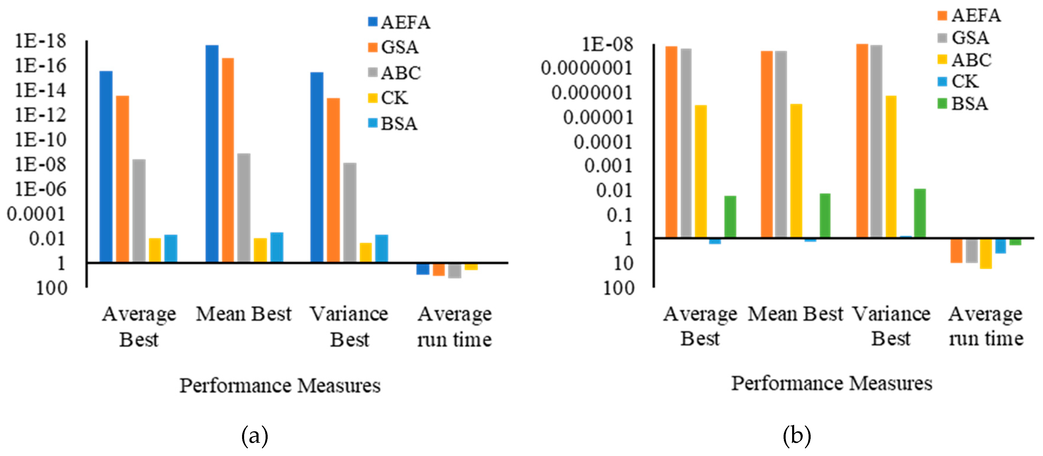
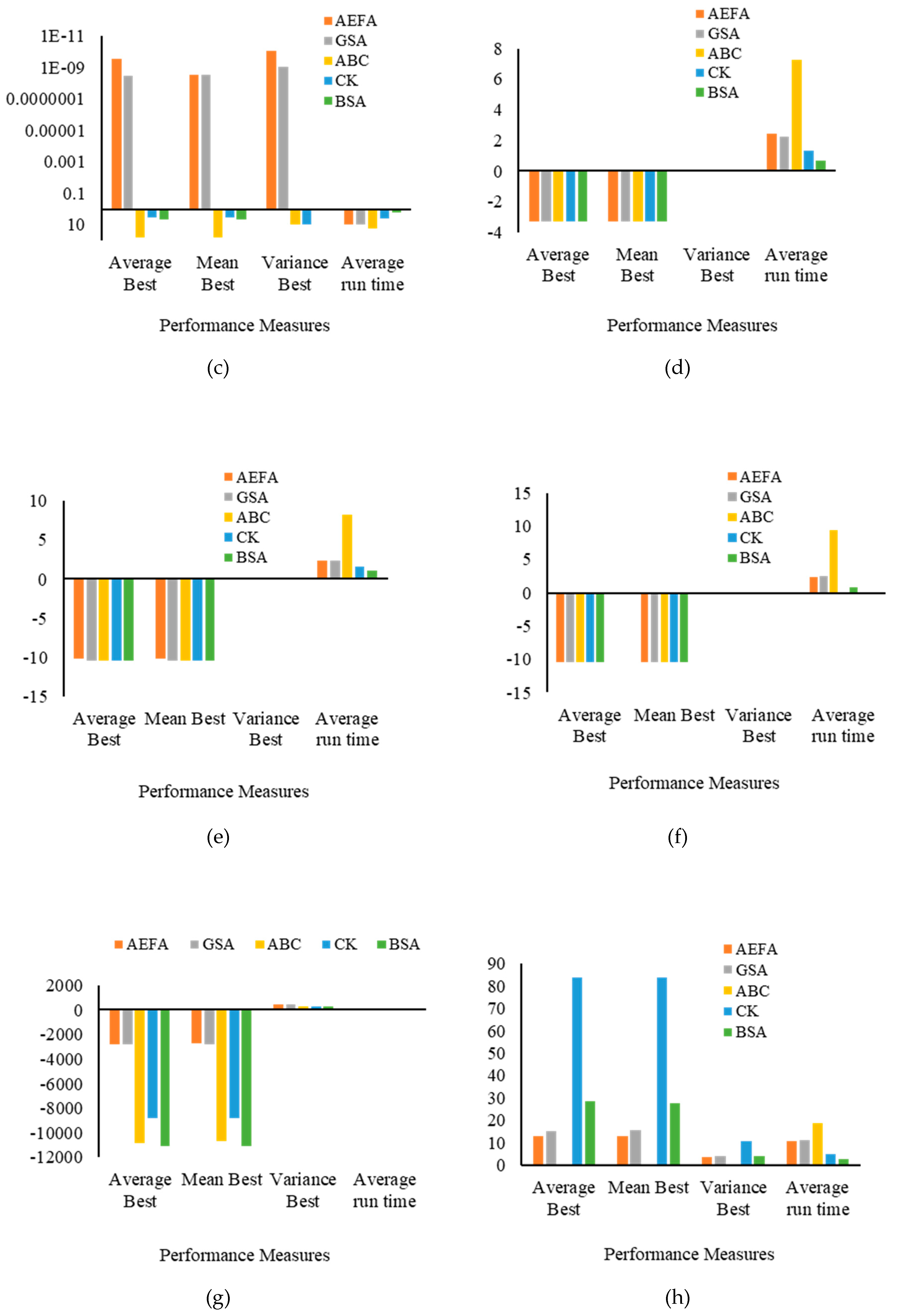
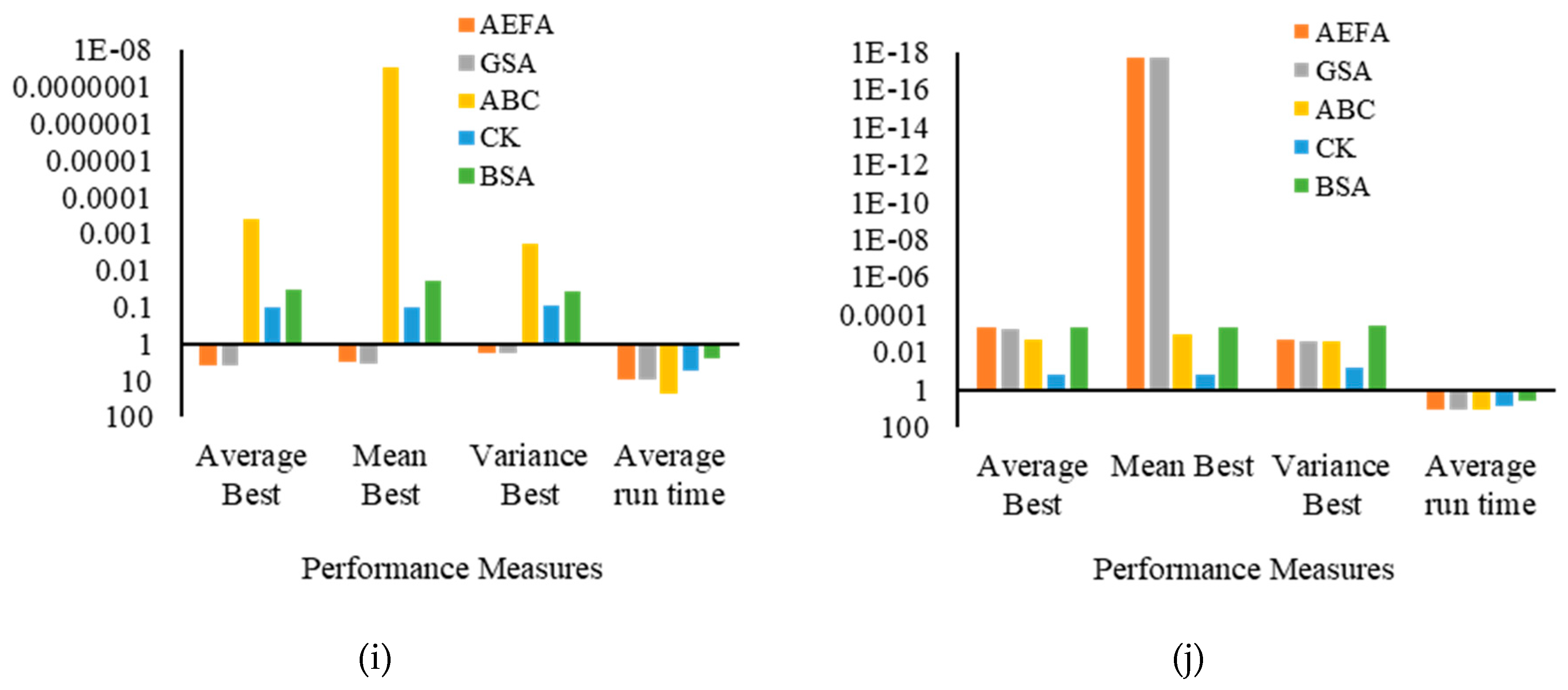
5.1. Performance Comparison of the AEFA With Existing Evolutionary Approaches
5.1.1. Parameter Setting
5.1.2. Results and Discussion
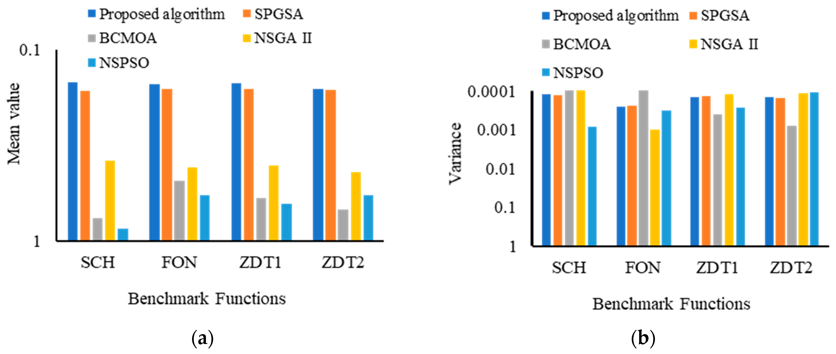
5.2. Performance Comparison of the Proposed Algorithm with Existing Multi-Objective Optimization Algorithms
5.2.1. Parameter Setting
5.2.2. Results and Discussion
5.3. Sensitivity Analysis of the Proposed Algorithm
Results and Discussion
6. Conclusions and Future Work
Author Contributions
Funding
Conflicts of Interest
References
- Nobahari, H.; Nikusokhan, M.; Siarry, P. Non-dominated sorting gravitational search algorithm. In Proceedings of the 2011 International Conference on Swarm Intelligence, Cergy, France, 14–15 June 2011; pp. 1–10. [Google Scholar]
- Van Veldhuizen, D.A.; Lamont, G.B. On measuring multiobjective evolutionary algorithm performance. In Proceedings of the 2000 Congress on Evolutionary Computation, La Jolla, CA, USA, 16–19 July 2000; Volume 1, pp. 204–211. [Google Scholar]
- Deb, K.; Pratap, A.; Agarwal, S.; Meyarivan, T. A fast and elitist multiobjective genetic algorithm: NSGA-II. IEEE Trans. Evol. Comput. 2002, 6, 182–197. [Google Scholar] [CrossRef]
- Zhao, B.; Cao, Y.J. Multiple Objective Particle Swarm Optimization Technique for Economic Load Dispatch. J. Zhejiang Univ. Sci. A 2005, 6, 420–427. [Google Scholar]
- Cagnina, L. A Particle Swarm Optimizer for Multi-Objective Optimization. J. Comput. Sci. Technol. 2005, 5, 204–210. [Google Scholar]
- Zhang, Y.; Gong, D.W.; Ding, Z. A bare-bones multi-objective particle swarm optimization algorithm for environmental/economic dispatch. Inf. Sci. 2012, 192, 213–227. [Google Scholar] [CrossRef]
- Li, X. A non-dominated sorting particle swarm optimizer for multiobjective optimization. In Genetic and Evolutionary Computation Conference; Springer: Berlin/Heidelberg, Germany, 2003; pp. 37–48. [Google Scholar]
- Yadav, A. AEFA: Artificial electric field algorithm for global optimization. Swarm Evol. Comput. 2019, 48, 93–108. [Google Scholar]
- Demirören, A.; Hekimoğlu, B.; Ekinci, S.; Kaya, S. Artificial Electric Field Algorithm for Determining Controller Parameters in AVR system. In Proceedings of the 2019 International Artificial Intelligence and Data Processing Symposium (IDAP), Malatya, Turkey, 21–22 September 2019; pp. 1–7. [Google Scholar]
- Abdelsalam, A.A.; Gabbar, H.A. Shunt Capacitors Optimal Placement in Distribution Networks Using Artificial Electric Field Algorithm. In Proceedings of the 2019 the 7th International Conference on Smart Energy Grid Engineering (SEGE), Oshawa, ON, Canada, 12–14 August 2019; pp. 77–85. [Google Scholar]
- Shafik, M.B.; Rashed, G.I.; Chen, H. Optimizing Energy Savings and Operation of Active Distribution Networks Utilizing Hybrid Energy Resources and Soft Open points: Case Study in Sohag, Egypt. IEEE Access 2020, 8, 28704–28717. [Google Scholar] [CrossRef]
- Thakur, M.; Meghwani, S.S.; Jalota, H. A modified real coded genetic algorithm for constrained optimization. Appl. Math. Comput. 2014, 235, 292–317. [Google Scholar] [CrossRef]
- Gong, M.; Jiao, L.; Du, H.; Bo, L. Multiobjective immune algorithm with nondominated neighbor-based selection. Evol. Comput. 2008, 16, 225–255. [Google Scholar] [CrossRef]
- Liu, Y.; Niu, B.; Luo, Y. Hybrid learning particle swarm optimizer with genetic disturbance. Neurocomputing 2015, 151, 1237–1247. [Google Scholar] [CrossRef]
- Fonseca, C.M.; Fleming, P.J. Genetic algorithms for multi-objective optimization: Formulation, discussion and generalization. In Proceedings of the 5th International Conference on Genetic Algorithms, San Mateo, CA, USA, 1 June 1993; pp. 416–423. [Google Scholar]
- Horn, J.; Nafploitis, N.; Goldberg, D.E. A niched Pareto genetic algorithm for multi-objective optimization. In Proceedings of the 1st IEEE Conference on Evolutionary Computation, Orlando, FL, USA, 27–29 June 1994; pp. 82–87. [Google Scholar]
- Tan, K.C.; Goh, C.K.; Mamun, A.A.; Ei, E.Z. An evolutionary artificial immune system for multi-objective optimization. Eur. J. Oper. Res. 2008, 187, 371–392. [Google Scholar] [CrossRef]
- Zitzler, E. Evolutionary Algorithms for Multiobjective Optimization: Methods and Applications; Ithaca: Shaker, OH, USA, 1999; Volume 63. [Google Scholar]
- Srinivas, N.; Deb, K. Multi-Objective function optimization using non-dominated sorting genetic algorithms. Evol. Comput. 1995, 2, 221–248. [Google Scholar] [CrossRef]
- Zitzler, E.; Thiele, L. Multiobjective optimization using evolutionary algorithms—A comparative case study. In International Conference on Parallel Problem Solving from Nature; Springer: Berlin/Heidelberg, Germany, 1998; pp. 292–301. [Google Scholar]
- Rudolph, G. Technical Report No. CI-67/99: Evolutionary Search under Partially Ordered Sets; Dortmund Department of Computer Science/LS11, University of Dortmund: Dortmund, Germany, 1999. [Google Scholar]
- Rughooputh, H.C.; King, R.A. Environmental/economic dispatch of thermal units using an elitist multiobjective evolutionary algorithm. In Proceedings of the IEEE International Conference on Industrial Technology, Maribor, Slovenia, 10–12 December 2003; Volume 1, pp. 48–53. [Google Scholar]
- Deb, K. Multi-Objective Optimization Using Evolutionary Algorithms; John Wiley & Sons: New York, NY, USA, 2001; Volume 16. [Google Scholar]
- Vrugt, J.A.; Robinson, B.A. Improved evolutionary optimization from genetically adaptive multimethod search. Proc. Natl. Acad. Sci. USA 2007, 104, 708–711. [Google Scholar] [CrossRef] [PubMed]
- Deb, K.; Jain, H. An evolutionary many-objective optimization algorithm using reference-point-based nondominated sorting approach, part I: Solving problems with box constraints. IEEE Trans. Evol. Comput. 2013, 18, 577–601. [Google Scholar] [CrossRef]
- Jain, H.; Deb, K. An evolutionary many-objective optimization algorithm using reference-point based nondominated sorting approach, part II: Handling constraints and extending to an adaptive approach. IEEE Trans. Evol. Comput. 2013, 18, 602–622. [Google Scholar] [CrossRef]
- Zhao, B.; Guo, C.X.; Cao, Y.J. A multiagent-based particle swarm optimization approach for optimal reactive power dispatch. IEEE Trans. Power Syst. 2005, 20, 1070–1078. [Google Scholar] [CrossRef]
- Zhang, Q.; Li, H. MOEA/D: A multiobjective evolutionary algorithm based on decomposition. IEEE Trans. Evol. Comput. 2007, 11, 712–731. [Google Scholar] [CrossRef]
- Ma, X.; Liu, F.; Qi, Y.; Li, L.; Jiao, L.; Liu, M.; Wu, J. MOEA/D with Baldwinian learning inspired by the regularity property of continuous multiobjective problem. Neurocomputing 2014, 145, 336–352. [Google Scholar] [CrossRef]
- Martinez, S.Z.; Coello, C.A.C. A multi-objective evolutionary algorithm based on decomposition for constrained multi-objective optimization. In Proceedings of the 2014 IEEE Congress on Evolutionary Computation (CEC), Beijing, China, 6–11 July 2014; pp. 429–436. [Google Scholar]
- Gu, F.; Liu, H.L.; Tan, K.C. A multiobjective evolutionary algorithm using dynamic weight design method. Int. J. Innov. Comput. Inf. Control 2012, 8, 3677–3688. [Google Scholar]
- Zhang, X.; Tian, Y.; Cheng, R.; Jin, Y. An efficient approach to nondominated sorting for evolutionary multiobjective optimization. IEEE Trans. Evol. Comput. 2014, 19, 201–213. [Google Scholar] [CrossRef]
- Chong, J.K.; Qiu, X. An Opposition-Based Self-Adaptive Differential Evolution with Decomposition for Solving the Multiobjective Multiple Salesman Problem. In Proceedings of the 2016 IEEE Congress on Evolutionary Computation (CEC), Vancouver, BC, Canada, 24–29 July 2016; pp. 4096–4103. [Google Scholar]
- Cheng, R.; Jin, Y.; Olhofer, M.; Sendhoff, B. A reference vector guided evolutionary algorithm for many-objective optimization. IEEE Trans. Evol. Comput. 2016, 20, 773–791. [Google Scholar] [CrossRef]
- Hassanzadeh, H.R.; Rouhani, M. A multi-objective gravitational search algorithm. In Proceedings of the 2010 2nd International Conference on Computational Intelligence, Communication Systems and Networks, Liverpool, UK, 28–30 July 2010; pp. 7–12. [Google Scholar]
- Yuan, X.; Chen, Z.; Yuan, Y.; Huang, Y.; Zhang, X. A strength pareto gravitational search algorithm for multi-objective optimization problems. Int. J. Pattern Recognit. Artif. Intell. 2015, 29, 1559010. [Google Scholar] [CrossRef]
- Li, M.; Yang, S.; Liu, X. Shift-based density estimation for Pareto-based algorithms in many-objective optimization. IEEE Trans. Evol. Comput. 2013, 18, 348–365. [Google Scholar] [CrossRef]
- Zitzler, E.; Laumanns, M.; Thiele, L. TIK report 103: SPEA2: Improving the Strength Pareto Evolutionary Algorithm; Computer Engineering and Networks Laboratory (TIK), ETH Zurich: Zurich, Switzerland, 2001. [Google Scholar]
- Schott, J.R. Fault Tolerant Design Using Single and Multicriteria Genetic Algorithm Optimization; Air force inst of tech Wright-Patterson AFB: Cambridge, MA, USA, 1995. [Google Scholar]
- Guzmán, M.A.; Delgado, A.; De Carvalho, J. A novel multiobjective optimization algorithm based on bacterial chemotaxis. Eng. Appl. Artif. Intell. 2010, 23, 292–301. [Google Scholar] [CrossRef]


| Author(s) | Objective/Work Done | Technique Proposed/Used | Performance Parameters | Research Gap(s) Identified |
|---|---|---|---|---|
| Nobahari, et.al. [1] | Proposed a multi-objective gravitational search based on non-dominated sorting for power transformer design | Non-dominated sorting gravitational search algorithm (NSGSA) | Normalized arithmetic mean | The Algorithm lacks scalability when dealing with complex cases of power transformer design. |
| Srinivas, and Deb [19] | Proposed a multi-objective genetic algorithm based on non-dominated sorting | Non-dominated sorting genetic algorithm (NSGA) | Chi-square test | The proposed algorithm shows a slow convergence rate. |
| Deb and Jain [25] | Proposed an evolutionary approach for solving many-objective optimization | Reference-based non dominated sorting approach (NSGA3) |
| Recombination operator can be improved to enhance population diversity |
| Zhang and Li [28] | Proposed a multi-objective evolutionary algorithm based on decomposition | The multi-objective evolutionary algorithm based on decomposition (MOEA/D) |
| The penalty parameter used in the proposed algorithm is statically initialized. For an extremely lower or higher value, the performance of the penalty method decreases |
| Martinez and Coello [30] | Proposed a decomposition-based multi-objective evolutionary algorithm (eMOEA/D-DE) for constraint MOOP | A new selection mechanism based on -constraint method |
| Constraint parameters used in the algorithm are statically initialized. It can be initialized dynamically. |
| Gu et.al. [31] | Proposed a multi-objective evolutionary algorithm based on the projection of the current non-dominated solutions and equidistance interpolation | Dynamic weight design method with MOEA/D |
| The algorithm lacks efficacy to solve complex higher-dimensional problems. |
| Zhang, et al. [32] | Proposed a novel and computationally efficient approach to non-dominated sorting | Efficient non-dominated sort (ENS) |
| The efficiency of the algorithm decreases with an increase in the number of objectives |
| Chong and Qiu [33] | Proposed MOO algorithm to solve multi-objective traveling salesman problem | Self-adaptive differential algorithm with a decomposition-based framework (D-OSADE) |
| The algorithm becomes less effective as the number of salesmen increases |
| Cheng et al. [34] | Proposed an evolutionary algorithm for many-objective optimization | Reference vector guided evolutionary algorithm (RVEA) |
| The reference vector is static. The selection type of reference vector to be used in many-objective optimization is not considered |
| Hassanzade and Rouhani [35] | Proposed a multi-objective algorithm based on gravitational force | Multi-objective gravitational search algorithm (MOGSA) |
| The algorithm suffers premature convergence in solving complex higher-dimensional problems. |
| Yuan et al. [36] | Proposed a multi-objective gravitational search based on the concept of strength Pareto | Strength Pareto gravitational search (SPGSA) |
| Population diversity can be further improved. |
| Symbol | Definition |
|---|---|
| Initial searching population size | |
| Searching population | |
| External population size | |
| External population | |
| Position of charged particle (candidate solution) in dimension at time | |
| velocity of charged particle in dimension at time | |
| Non-dominated set of charged particles (candidate solution) | |
| Objective fitness function | |
| Charged particle with best fitness at time | |
| Charged particle with worst fitness at time | |
| Coulomb’s constant | |
| Total charge on a charged particle at time | |
| Small charge of charged particle to determine the total charge acting on charged particle | |
| Force exerted by charge particle on charge particle | |
| Shift based density estimation | |
| Maximum number of iterations | |
| Distance between two non-dominated solutions ( and ) | |
| Shared crowding distance for each | |
| Shared crowding distance of chosen for deletion from the external population set |
| Benchmark Function | Type | Variable Bound | Objective Function | Dimension(s) |
|---|---|---|---|---|
| F1 | UM | 30 | ||
| F2 | UM | 30 | ||
| F3 | UM | 30 | ||
| F4 | LDMM | 6 | ||
| F5 | LDMM | 4 | ||
| F6 | LDMM | 4 | ||
| F7 | HDMM | 30 | ||
| F8 | HDMM | 30 | ||
| F9 | HDMM | 30 | ||
| F10 | HDMM | + + +, | 30 |
| Description | Parameter | Value |
|---|---|---|
| Population size | 50 | |
| Initial value used in Coulomb’s constant | 100 | |
| Maximum number of iterations | 300 for and 1000 for the rest of the benchmark functions |
| Benchmark | Optimization Algorithm | Statistical Performance Indices | |||
|---|---|---|---|---|---|
| Average Best | Mean Best | Variance Best | Average Run Time | ||
| F1 | AEFA | ||||
| GSA | |||||
| ABC | |||||
| CK | |||||
| BSA | |||||
| F2 | AEFA | ||||
| GSA | |||||
| ABC | |||||
| CK | |||||
| BSA | |||||
| F3 | AEFA | ||||
| GSA | |||||
| ABC | |||||
| CK | |||||
| BSA | |||||
| F4 | AEFA | ||||
| GSA | |||||
| ABC | |||||
| CK | |||||
| BSA | |||||
| F5 | AEFA | ||||
| GSA | |||||
| ABC | |||||
| CK | |||||
| BSA | |||||
| F6 | AEFA | ||||
| GSA | |||||
| ABC | |||||
| CK | |||||
| BSA | |||||
| F7 | AEFA | ||||
| GSA | |||||
| ABC | |||||
| CK | |||||
| BSA | |||||
| F8 | AEFA | ||||
| GSA | |||||
| ABC | |||||
| CK | |||||
| BSA | |||||
| F9 | AEFA | ||||
| GSA | |||||
| ABC | |||||
| CK | |||||
| BSA | |||||
| F10 | AEFA | ||||
| GSA | |||||
| ABC | |||||
| CK | |||||
| BSA | |||||
| Benchmark Function | Type | Variable Bound | Objective Function | Dimension(s) |
|---|---|---|---|---|
| SCH [3] | Bi-Objective (Low dimension) | Minimize | 1 | |
| Minimize | ||||
| FON [3] | Bi-Objective (Low dimension) | Minimize | 3 | |
| Minimize | ||||
| ZDT1 [3] | Bi-Objective (High dimension) | Minimize | 30 | |
| Minimize , | ||||
| ZDT2 [3] | Bi-Objective (High dimension) | Minimize | 30 | |
| Minimize , | ||||
| MOP5 [5] | Tri-Objective (Low dimension) | <=30 | Minimize | 2 |
| Minimize +15 | ||||
| Minimize | ||||
| MOP6 [5] | Bi-Objective (Low dimension) | <=1 | Minimize | 2 |
| Minimize | ||||
| DTLZT2 [13] | Tri-Objective (High dimension) | Minimize | 12 | |
| Minimize | ||||
| Minimize , where |
| Description | Parameter | Value |
|---|---|---|
| Population (charged particles) size | 100 | |
| External Population size | 100 for SCH, FON, ZDT 800 for MOP functions | |
| Initial value used in Coulomb’s constant | 100 | |
| The maximum number of iterations | 100 for SCH and FON functions 250 for ZDT and MOP functions | |
| Initial crossover probability | 1.0 | |
| Final crossover probability | 0.0 | |
| Initial mutation probability | 0.01 | |
| Final mutation probability | 0.001 |
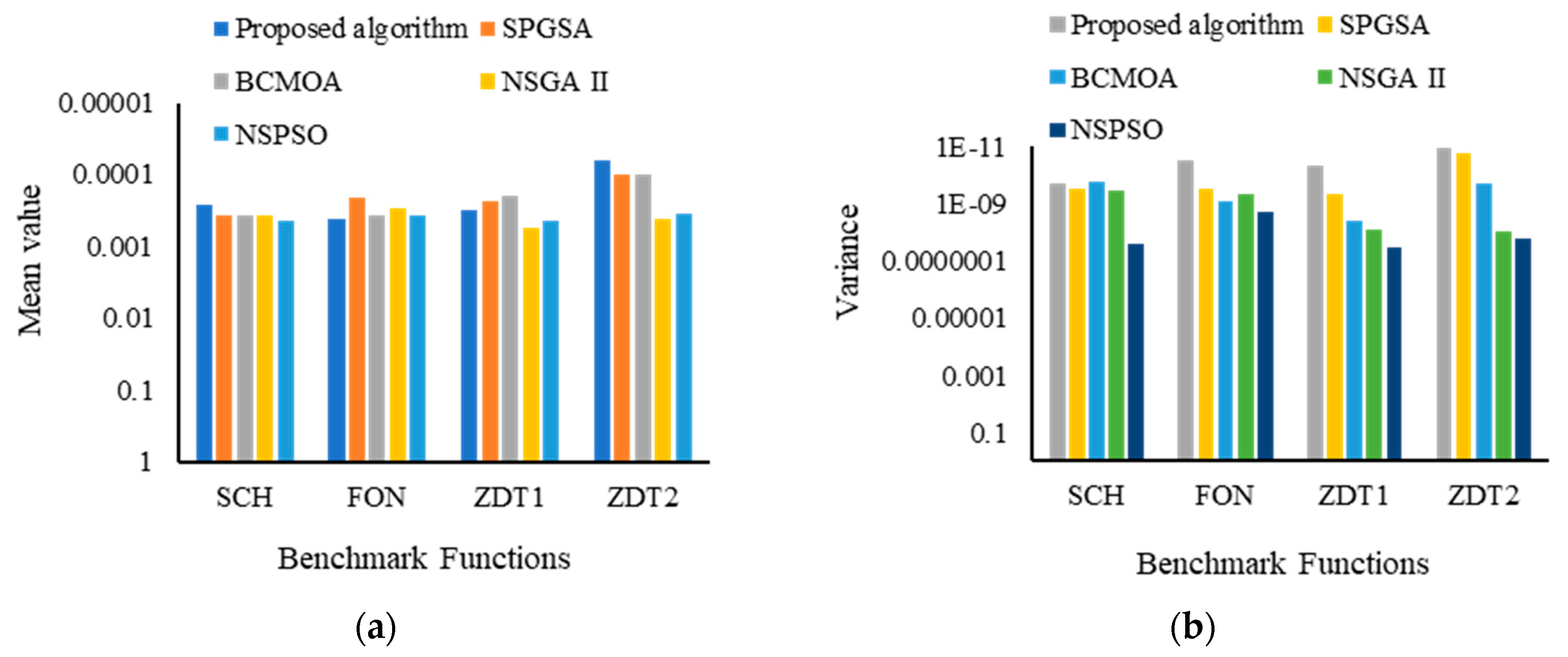
| Benchmark Function | Parameters | Algorithm | ||||
|---|---|---|---|---|---|---|
| Proposed Algorithm | SPGSA | BCMOA | NSGA II | NSPSO | ||
| SCH | Mean | |||||
| Variance | ||||||
| FON | Mean | |||||
| Variance | ||||||
| ZDT1 | Mean | |||||
| Variance | ||||||
| ZDT2 | Mean | |||||
| Variance | ||||||
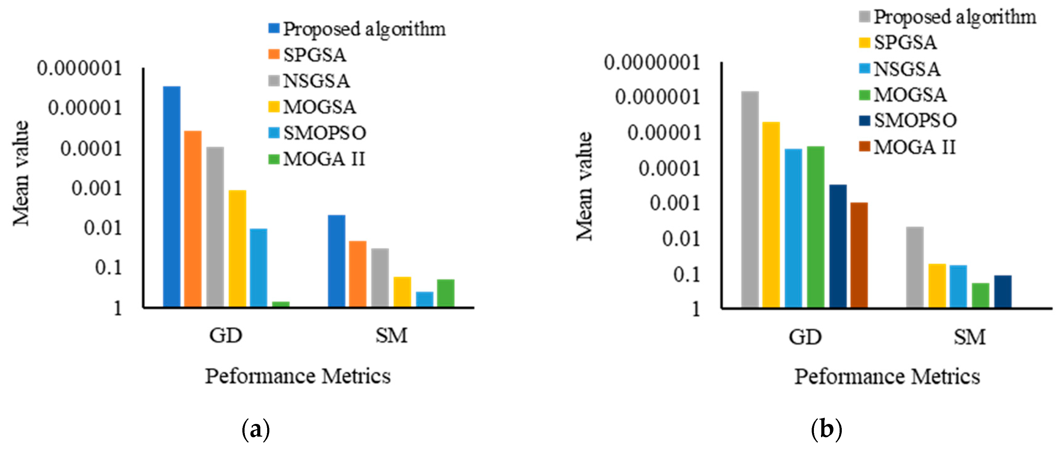
| Benchmark Function | Metric | Algorithm | |||||
|---|---|---|---|---|---|---|---|
| Proposed Algorithm | SPGSA | NSGSA | MOGSA | SMOPSO | MOGA II | ||
| MOP5 | GD | ||||||
| SM | |||||||
| MOP6 | GD | ||||||
| SM | |||||||
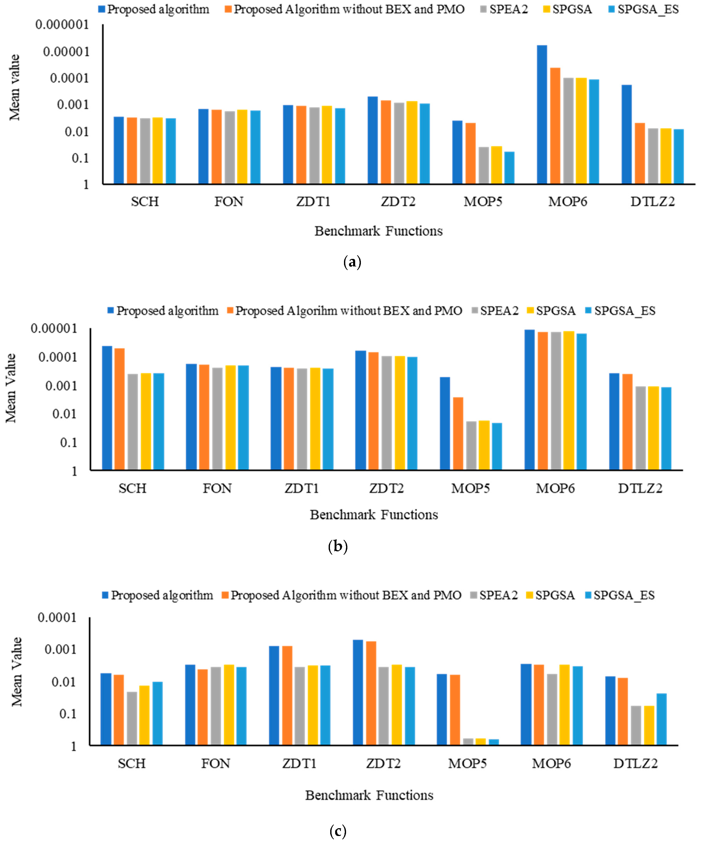
| Performance Metric | Benchmark Functions | Proposed Algorithm | SPEA2 | SPGSA | SPGSA_ES | |
|---|---|---|---|---|---|---|
| CM metric | SCH | |||||
| FON | ||||||
| ZDT1 | ||||||
| ZDT2 | ||||||
| MOP5 | ||||||
| MOP6 | ||||||
| DTLZ2 | ||||||
| GD metric | SCH | |||||
| FON | ||||||
| ZDT1 | ||||||
| ZDT2 | ||||||
| MOP5 | ||||||
| MOP6 | ||||||
| DTLZ2 | ||||||
| SM metric | SCH | 2 | ||||
| FON | ||||||
| ZDT1 | ||||||
| ZDT2 | ||||||
| MOP5 | ||||||
| MOP6 | ||||||
| DTLZ2 |
| Analysis | Sensitivity Analysis Performed on | Parameter Setting | Setting of Variable Parameters | Number of Parameter Setting Combinations |
|---|---|---|---|---|
| Sensitivity Analysis 1 |
|
|
| 30 |
| Sensitivity Analysis 2 | Initial population Size | Mutation probability = 0.001 | Population Size = 50; 100; 200; 400; 500 | 20 |
| Maximum no. of Iterations | Crossover probability = 1.0 | Maximum no. of Iterations = 500; 1000; 2000 | 50 |
| Performance Measures | Overall Performance of Parameter Setting Combinations | ||||
|---|---|---|---|---|---|
| Very Good | Good | Average | Poor | Very Poor | |
| Combined performance Score | 5.0–4.0 | 4.0–3.0 | 3.0–2.0 | 2.0–1.0 | 1.0–0.0 |
| Value of Mutation Parameter | Value of Constant Parameters | Metrics | Combined Performance Score | Overall Performance | |
|---|---|---|---|---|---|
| GD | SM | ||||
| 0.01 |
| 3899 | 24.6 | 2.9 | Average |
| 0.07 | 67 | 32.3 | 3.6 | Good | |
| 0.09 | 86 | 33.5 | 3.0 | Average | |
| 0.001 | 135 | 28.4 | 1.8 | Very Poor | |
| 0.01 |
| 11,085 | 22 | 3.3 | Good |
| 0.07 | 55 | 32 | 3.8 | Good | |
| 0.09 | 83 | 28.7 | 2.6 | Average | |
| 0.001 | 71 | 32 | 3.4 | Good | |
| Value of Crossover Parameter | Value of Constant Parameters | Metrics | Combined Performance Score | Overall Performance | |
|---|---|---|---|---|---|
| GD | SM | ||||
| 0.7 |
| 112 | 39 | 4.2 | Very Good |
| 0.8 | 45 | 28 | 3.2 | Good | |
| 0.9 | 60 | 35 | 3.0 | Average | |
| 1.0 | 36 | 30 | 2.6 | Average | |
| 0.7 |
| 4454 | 26 | 3.8 | Good |
| 0.8 | 10,121 | 23 | 3.6 | Good | |
| 0.9 | 3632 | 21 | 3.2 | Good | |
| 1.0 | 11,068 | 24 | 3 | Good | |
| Initial Population Size | Value of Constant Parameters | Metrics | Combined Performance Score | Overall Performance | |
|---|---|---|---|---|---|
| GD | SM | ||||
| 100 |
| 225 | 28 | 3.0 | Average |
| 200 | 32 | 34 | 3.1 | Good | |
| 400 | 36 | 39 | 4.0 | Very Good | |
| 500 | 38 | 30 | 3.6 | Good | |
| 100 |
| 60 | 30 | 3.5 | Good |
| 200 | 105 | 34 | 3.9 | Good | |
| 400 | 21 | 36 | 3.5 | Good | |
| 500 | 21 | 35 | 3.2 | Good | |
| Maximum No of Iterations | Value of Constant Parameters | Metrics | Combined Performance Score | Overall Performance | |
|---|---|---|---|---|---|
| GD | SM | ||||
| 500 |
| 65 | 30 | 3.4 | Good |
| 1000 | 21 | 33 | 3.2 | Good | |
| 2000 | 30 | 34 | 3.2 | Good | |
| 500 |
| 50 | 32 | 3.3 | Good |
| 1000 | 51 | 34 | 3.6 | Good | |
| 2000 | 24 | 34 | 3.8 | Good | |
| Initial Value of Coulomb’s Constant | Value of Constant Parameters | Metrics | Combined Performance Score | Overall Performance | |
|---|---|---|---|---|---|
| GD | SM | ||||
| 100 |
| 85 | 31 | 3.6 | Good |
| 300 | 30 | 40 | 3.3 | Good | |
| 500 | 40 | 332 | 4.2 | Very Good | |
| 100 |
| 62 | 35 | 3.3 | Good |
| 300 | 48 | 39 | 3.9 | Good | |
| 500 | 38 | 31 | 4.0 | Very Good | |
© 2020 by the authors. Licensee MDPI, Basel, Switzerland. This article is an open access article distributed under the terms and conditions of the Creative Commons Attribution (CC BY) license (http://creativecommons.org/licenses/by/4.0/).
Share and Cite
Petwal, H.; Rani, R. An Improved Artificial Electric Field Algorithm for Multi-Objective Optimization. Processes 2020, 8, 584. https://doi.org/10.3390/pr8050584
Petwal H, Rani R. An Improved Artificial Electric Field Algorithm for Multi-Objective Optimization. Processes. 2020; 8(5):584. https://doi.org/10.3390/pr8050584
Chicago/Turabian StylePetwal, Hemant, and Rinkle Rani. 2020. "An Improved Artificial Electric Field Algorithm for Multi-Objective Optimization" Processes 8, no. 5: 584. https://doi.org/10.3390/pr8050584
APA StylePetwal, H., & Rani, R. (2020). An Improved Artificial Electric Field Algorithm for Multi-Objective Optimization. Processes, 8(5), 584. https://doi.org/10.3390/pr8050584