1. Introduction
Bioelectrochemical Systems (BES) technology has been of significant interest recently due to the advantage of producing energy from renewable organic materials. Mainly, Microbial Electrochemical Cells (MXC) have gained attention among BES due to its capacity to treat wastewater and simultaneously recover energy [
1,
2].
MXC processes take advantage of Anode-Respiring Bacteria (ARB) applied in electrochemical systems. During the respiration process, an electrical current is produced, and it is used in one way or another for producing energy depending on the type of MXC system. Two processes among them have received significant attention from many researchers in the last two decades due to the technological and economical advantages obtained from electricity generation in the case of Microbial Fuel Cells (MFC) and hydrogen production in the case of Microbial Electrolysis Cells (MEC). The current produced in the MFC system is used for the reduction of oxidized compounds (mainly oxygen); in MEC systems, the current is used to produce hydrogen gas [
3,
4]. In this sense, the MEC process has been recently considered as a promising renewable energy alternative to fossil fuels.
An MEC is an electrochemical system that generates hydrogen and removes organic matter from wastewater with the help of an externally-applied potential and the activity of exoelectrogens microorganisms. The microorganisms oxidize the organic matter and transfer the electrons outside their cells as a part of their respiration process. The released electrons go to the anode, where the applied potential increases their energy level. Simultaneously, protons are released at the anode and transferred to the cathode through the bulk phase or a membrane (if any). Finally, the electrons carry out the reduction of protons at the cathode. Due to the activity of microorganisms, in theory, it is necessary to apply externally only 135 mV to produce the hydrogen, which is considerably lower than the 1210 mV thermodynamically required by the classical electrolysis of water [
5,
6]. Hence, the advantages of MEC are the lower voltage needed for the H
2 generation and the removal of organic matter from wastewater.
The performance of BES depends on several electrochemical, physical-chemical, and biological factors. The understanding of the dynamic relations among these is critical to making this technology more efficient [
7,
8,
9]. Furthermore, the mathematical description of these relations is fundamental to the design and optimization of this kind of process [
10,
11]. Indeed, modeling of MXC processes has been an active area throughout the last decade. Recently, a broad classification of mathematical models of BES systems has been reported by Gadkari et al. [
12]. Nevertheless, most contributions are mainly focused on MFC, while modeling research work on MEC systems is still limited [
10,
12]. In any case, differential equations are used as the main mathematical tools for describing MXC systems.
Based on a previously-reported MFC model, Pinto et al. [
13] described a MEC system through a set of eight Ordinary Differential Equations (ODE) [
14]. The mathematical description includes: (i) a microbial multi-population dynamic (anodophilic, fermentative, methanogenic acetoclastic, and methanogenic hydrogenophilic microorganisms); (ii) a simplification of anaerobic degradation of wastewater based on two single steps (hydrolysis and fermentation); (iii) Bernard’s anaerobic digestion kinetics [
15]; and (iv) hydrogen consumption and production. Afterward, the MEC model was modified with additional considerations intended for a unified description of both MFC and MEC systems [
16]. In both models, there is not a dynamical description of biofilm.
On the other hand, based on a previously-reported MFC model [
17], Alavijeh et al. [
18] described a one-dimensional MEC system through a set of Partial Differential Equations (PDE). The model considers several variables of liquid bulk and biofilm, such as: (i) a microbial multi-population dynamic (anodophilic, fermentative, and methanogenic acetoclastic microorganisms); (ii) active and inactive microorganisms; (iii) spatial one-dimensional description of substrates and local potential in the biofilm; (iv) a one-dimensional dynamical description of biofilm thickness; (v) global dynamical description of substrates in the liquid bulk. The model provides a detailed description of the MEC system. Nevertheless, despite the model being simplified with linear boundary conditions, the numerical solution involves solving the nonlinear, time-dependent, and coupled system of partial and ordinary differential equations. Then, the numerical solution requires numerical in-out cycles among several numerical methods (trust-region-reflective method, Runge–Kutta–Fehlberg method, and Gear’s method).
After that, Mardanpour and Yaghmaei [
19] proposed a dynamic mathematical model to study microfluidic MEC systems with potential application in biohydrogen production for implantable medical devices. The mathematical description includes: (i) one microbial population dynamic; (ii) active and inactive microorganisms; (iii) one-dimensional local electrical potential description. Despite a detailed description of microbial biomass particles, there is not a differential equation related to biofilm thickness; instead, an algebraic equation for biofilm thickness is presented. The model provides an accurate description of the dynamical MEC system; however, it is limited to microfluidic applications.
Recently, Hussain et al. [
20] described the MEC system as a simple MEC Equivalent Electrical Circuit (EEC) model. Two first order differential equations were proposed to represent the voltage dynamics of internal capacitors of the EEC. The main advantage of this proposal is the online procedure for estimating EEC model parameters. Indeed, the approach can be used to achieve real-time monitoring of the MEC system. Despite variation in chemical oxygen demand concentration being captured by the proposed monitoring method, non-information of the microorganism and biofilm dynamics was described.
Mathematical models that take into account biofilm growth dynamics of a mixed microbial population, without the drawback of high computational resources in the model simulation, should be advantageous in the MEC system for optimization and control purposes. However, to the best of our knowledge, a mathematical MEC model based on those ideas has not been reported. In this work, we propose a dynamical model for an MEC with an emphasis on biofilm growth dynamics of a mixed population of microbes and biofilm processes such as the substrate diffusion, the potential loss, and the detachment of biomass. To avoid high computational resources in the MEC model simulation, the dynamical behavior of substrate distribution and potential inside the biofilm (PDE) are included in a set of ODE systems using average reaction rates.
The paper is organized as follows: the general MEC process is described in
Section 2. Then, the proposed dynamical model is shown in
Section 3. The implementation via simulation runs of the model for two study cases, chronoamperometry and voltammetry, is addressed in
Section 4. In
Section 5, some potential application and further comments are provided. Finally, some concluding remarks are presented in
Section 6.
2. The Cell
In this work, an MEC system composed of two chambers, the anodic and the cathodic one, separated by an ionic membrane is considered. Both of them are assumed under anaerobic conditions to avoid the oxygen being the final electron acceptor.
In the anodic chamber, there is an electrode in which the biomass attaches and creates a microbial film (named the bioanode). The biofilm takes the nutrients from the bulk phase in the anodic chamber and produces the electrons that travel externally to the cathode. Bacteria are capable of transferring electrons outside the cell, either directly or by endogenous mediators (which can also be added), named exoelectrogens [
3]. These latter include a wealth of genera such as Geobacter, Shewanella, Pseudomonas, and others [
21].
The absence of substances that can be final electron acceptors (e.g., sulfates, nitrates, metal cations, etc.) is assumed. Protons are also bio-products, and they travel to the cathodic chamber through the membrane, commonly Nafion; a proton exchange membrane [
5,
21,
22,
23].
The produced electrons pass through an external potential, which increases their energy level, and finally go to the cathode. If they have adequate potential, the protons coming from the solution in the anodic chamber are reduced, and the molecular hydrogen is produced.
Regarding the produced electrons, there is an open question related to the transference of electrons from the microbial cell to the anode. Rozendal et al. [
22] stated that this is either by direct contact with an electrode surface or aided by excreted redox mediators. The most recent studies have shown that the mechanisms for the electron transfer rely on the type of microorganism [
24].
3. Dynamical Model
The model was obtained from a time-dependent mass balance of the different species in the biofilm and the anodic chamber. In the biofilm, a mass balance was also made for the spatial distribution of substrate and a charge balance for the potential spatial distribution. For the applied potential, the anode was considered the working electrode.
3.1. The System
Each of the two chambers contained a volume of fluid
(mL) for the anodic one and
(mL) for the cathodic one, respectively. The anode chamber was fed continuously with a volumetric flow
F (mL d
−1). It was considered that the supplied solution was composed of a phosphate buffer (pH = 7.0) containing oligo-elements [
21,
22] and acetate as the only carbon source with a concentration
(mmol
mL
−1). The anode had an active area
(cm
2) where the microorganisms attached and created a uniform biofilm of thickness
(cm). The cathodic chamber contained only an abiotic buffered solution (pH = 7.0).
The electrodes were externally connected by a potentiometer that kept the potential (V) vs. the reference of the anode constant. It was assumed that the reference electrode and the anode were close enough that the ohmic losses between them were negligible.
3.2. Biomass
As the only carbon source was acetate, just two populations were considered in the system: the methanogenic and the exoelectrogens microorganisms. Both of them competed for the substrate and space in the biofilm.
Due to the absence of molecular hydrogen in the anodic chamber, the methane was produced by the acetoclastic process as follows:
The exoelectrogens microorganisms carried out the following reaction:
The microorganisms used part of the produced electrons for self-growth and their own energy production [
25]; this fraction is denoted as
, and it was assumed that the rest of the fraction,
, was expelled directly to the anode.
It was considered that all the microorganisms were attached to the biofilm and there was no activity in the liquid phase. The concentration in the biofilm was (mg VS cm−2) for the acetoclastic methanogens and (mg VS cm−2) for the exoelectrogens microorganisms, where (mg) stands for the measurement of the biomass as volatile solids.
3.3. Biological Reaction Pathways
The considered biological reactions were acetoclastic methanogenesis (with a reaction rate
):
electrogenesis (with a reaction rate
:
and self-oxidation of biomass through endogenous respiration (with a reaction rate
:
where
(
) are the respective yield coefficients. In the ideal case, when no biomass was produced and all the substrate was oxidized, their values were obtained from carbon and electron balances. For details, see
Appendix A.
3.4. Microorganisms’ Kinetics
The rate at which methanogenic microorganisms consumed the substrate follows the Haldane kinetics [
15]:
where
is the maximum specific growth rate without inhibition (mmol S mg VS
−1 d
−1),
is the half maximum rate concentration of
S without inhibition (mmol S mL
−1), and
is the inhibition constant associated with
S (mmol S mL
−1).
The growth of the exoelectrogens microorganisms was affected by the substrate concentration and the potential of the anode (which can be seen as the electron acceptor). The rate is described by the multiplicative Nernst–Monod kinetics [
17,
26]:
where:
is the maximum rate of utilization by the exoelectrogens microorganisms (mmol S mg VS
−1 d
−1),
S is the acetate concentration (mmol S mL
−1),
is the half-maximum-rate-concentration of species
S (mmol S mL
−1),
(V) is the anode potential, and
(V) is the potential at which
when
. Both potentials are expressed vs. the same reference electrode.
Besides the growth, there is a process by which the microorganisms die or stop working. This process is the inactivation of active biomass, and it was considered that it followed the next kinetics [
17,
27]:
where
is the inactivation rate, and
(d
−1) is the inactivation constant, and it is assumed to be equal for both microbial populations. Notice that
can also be defined as a function of the medium characteristics (pH,
T, the presence of other substances); hence,
could be a time-dependent parameter for a batch reactor where the qualities of the medium may change with time. However, for this work, it is considered constant.
The endogenous respiration is related to the self-oxidation of exoelectrogens microorganisms [
17], and it is described using the Nernst–Monod equation:
where
(d
−1) is the endogenous decay coefficient.
3.5. Biofilm
The biofilm was composed of three different species: the two active microorganisms and ; and the inert biomass (mg VS cm−2). The latter is due to the inactive microorganisms, extracellular polymeric substances, etc.
The total volume (cm
3) of the biofilm was:
and its mass (mg) was:
where
is the biofilm density (mg VS cm
−3); it was assumed to be constant and uniform through the film.
From the previous expressions, the concentration of each species in the biofilm can be calculated as follows:
where
and
are the mass fractions of
and
, respectively.
It was assumed that there was no spatial variation of biomass along the biofilm. However, the substrate concentration and the potential can vary inside the film due to the mass and charge transfers [
17]. To find these variations, some balances were made for the acetate and electrons. It was assumed that all the transfers were unidirectional (axis
z) and perpendicular to the anode area. The anode surface was defined at
, and the interface between the biofilm and the liquid phase was located at
.
3.5.1. Substrate Diffusion
As the acetate reacted, a concentration gradient appeared along the biofilm thickness. Departing from the variation in the substrate concentration (
), the following mass balance can be established:
where
(mmol S cm
−2 d
−1) is the substrate flux in the
z-direction, i.e.,
with
(cm
−2 d
−1) the effective diffusion of the substrate in the biofilm. Due to the small thickness of the film, once the concentration of the substrate in the bulk changed, it was assumed that the distribution of
inside the biofilm immediately reached its steady state. Then, the previous equation can be expressed as:
Notice that the functions and are indeed Equations (1) and (2) evaluated on and .
Due to the absence of substrate diffusion to the electrode, the first boundary condition was:
It was assumed that there were no concentration gradients between the bulk and the biofilm surface. Then, the second boundary condition was:
where
S is the substrate concentration in the bulk of the anodic chamber.
3.5.2. Potential Losses
As the electrons flowed through the biofilm, there was a potential loss. The equation describing the potential variation
through the biofilm is:
where
is the flux of electrons (current density) in the
z-direction, i.e.,
Here, it was considered that electrons flowing through the biofilm immediately reached their steady-state. Then, the equation describing the potential variation through the biofilm is:
where
is the Faraday constant (96,487 mC mmol
);
is the conversion time factor (86,400 s d
−1);
(mS cm
−1 = mA V
−1 cm
−1) is the biofilm conductivity that can be seen as the sum of the effects related to the electrons’ transfer mechanisms.
The boundary conditions related to a fixed potential at the anode were:
Furthermore, it was assumed that electrons conducted only on the biofilm matrix; then, a second boundary condition was:
Thus, the substrate and the potential distribution along the biofilm,
and
, were obtained by solving Equations (
8) and (
9).
3.5.3. Detachment
It was assumed that the biofilm thickness was finite [
13,
28]. Then, there was a mechanism by which biomass was detached from the film and released into the bulk liquid. Thus, it was assumed that the rate of detachment
followed a second-order dependence on the biofilm thickness as follows [
29]:
where
is the detachment constant (cm
−1 d
−1), which can be dependent on the shear stress.
3.6. Mass Balances
3.6.1. Average Reaction Rates
Due to the mass and charge transfers, the active microorganisms along the biofilm were exposed to different substrate concentrations and potentials. Therefore, their growth and oxidation rates depended on the position inside the film. The reaction rates affected by the z-position in the biofilm were:
To find the average reaction rates, the previous expressions can be integrated along the biofilm as follows:
Notice that it cannot be expected that the average reaction rates are strictly as accurate as the complete local reaction rate profile; however, the proposed approach intended to capture the entire dynamic related to the reaction rate profile.
3.6.2. Global Balance of Species in the MEC
The dynamical behavior of the system was obtained from a mass balance of the different species: (i) substrate; (ii) biofilm; (iii) active acetoclastic biomass; and (iv) active exoelectrogens microorganisms.
The accumulation of the substrate inside the biofilm was neglected due to the small volume of the biofilm compared to the liquid phase. Then, the mass balance for the substrate can be expressed as:
A constant volume of the anodic chamber was assumed; then, the previous equation can be rearranged as:
The mass balance for the biofilm follows as:
The mass balance for the active acetoclastic biomass can be expressed as:
From the substitution of Equation (
15) in the previous equation, it is possible to obtain:
The mass balance for the active exoelectrogens microorganisms can be expressed as:
From the substitution of Equation (
15) in the previous equation, it is possible to obtain:
where the states of the MEC model are the substrate concentration in the liquid phase
S (g/L); the thickness of biomass in the film
(m); and the mass fractions of microorganisms
and
. The average reaction rates were obtained from the Equations (
11)–(
13). Then, their calculation required the integration of Equations (
8) and (
9) for each instant of time. For details about the integration method to solve this set of ordinary differential equations, see
Appendix B.
3.7. Current
Under the assumption that all the generated electrons go to the anode, the expected current
I (mA) was:
where
and
are constants.
3.8. Methane
Due to the low solubility of methane, it was assumed that this species passed directly to the gas phase of the anodic chamber once it was produced. The methane flow rate
(mmol CH
4 d
−1) was:
where
is a constant.
3.9. Hydrogen
The species of hydrogen considered were the proton H
+ and the molecular H
2. The protons were produced in the anodic chamber and traveled through the membrane to the cathode, where they were reduced:
The hydrogen flow rate
(mmolH
2 d
−1) was:
where
(dimensionless) was the overall efficiency of the cathode for the hydrogen production and
= 0.5 (mmol H
2 mEQ
−1).
It was assumed that once the molecular hydrogen was produced, it passed immediately to the gas phase in the cathodic chamber due to its low solubility in water.
4. Simulations
The simulations of the model were carried out in MATLAB (2018a, MathWorks, Natick, MA, USA, 2018). The system presented in the Equations (
14)–(
17) is considered to have the next form:
where
is the vector of states;
is the vector field;
is the vector of inputs; and
is the vector containing all the parameters of the model (such as those related to the kinetics, the thermodynamical constants, the yield coefficients, and the physical characteristics of the biofilm).
To integrate the system (
22) in a determined time span, it is necessary to define the parameters of
and the vector of initial conditions
. The vector of inputs must also be defined, and it can be a function of time. Two types of simulations were done, chronoamperometry and voltammetry, as described and discussed in the following subsections.
4.1. Chronoamperometry
In
Figure 1,
Figure 2,
Figure 3 and
Figure 4 are shown the dynamical behavior of the system for 30 days of numerical simulation in which step change perturbations in
and
were carried out as shown therein. The parameters and operating conditions are shown in
Table 1 and
Table 2. The initial operating condition for the simulation were:
= [2000 mg L
−1, 10 μm, 0.4, 0.3]
T. The following are some of the effects that can be observed in the simulations.
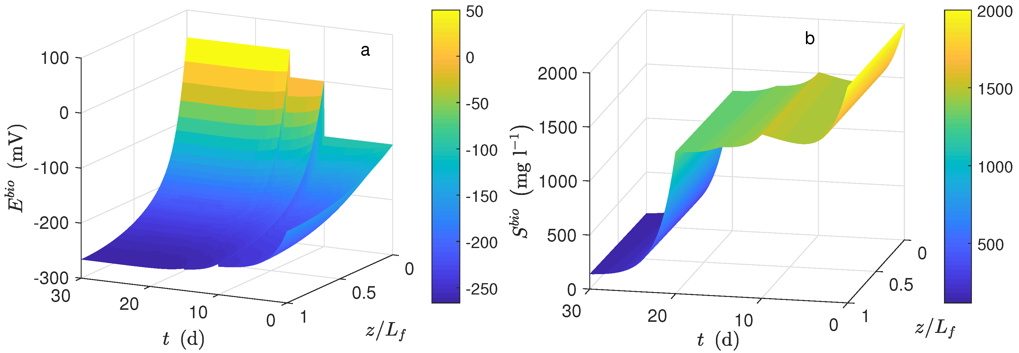
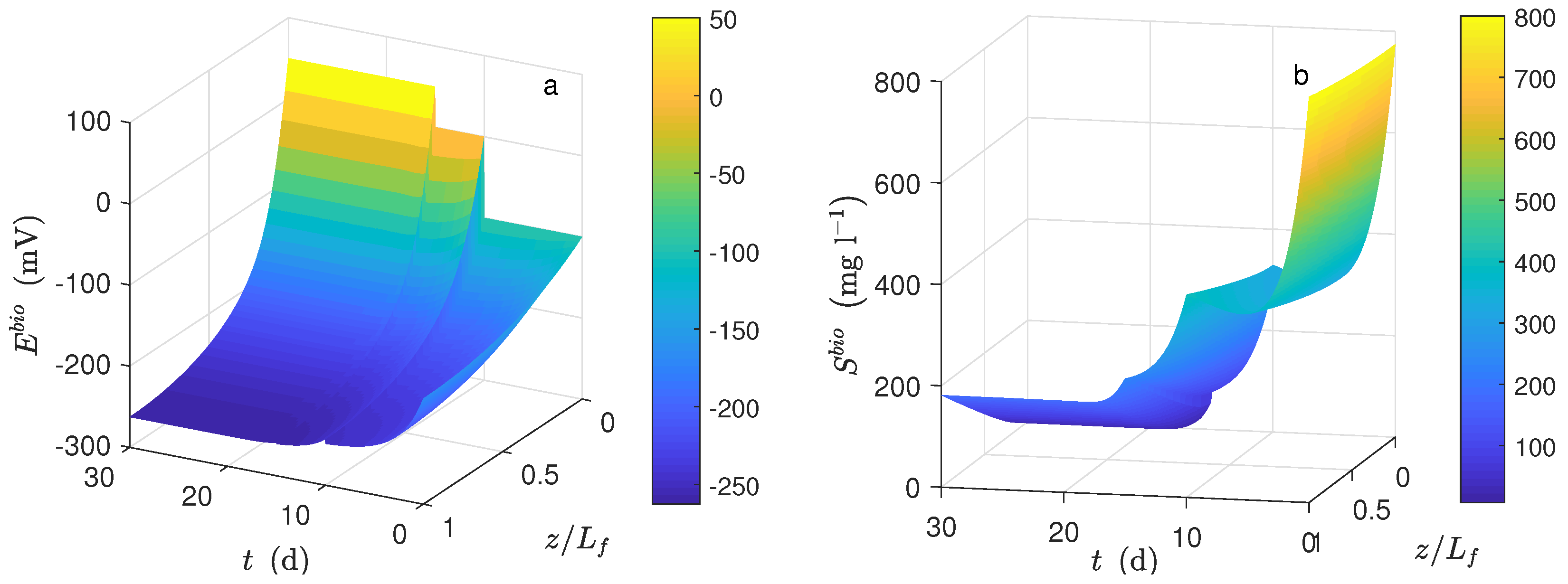
Figure 1a shows the dynamical behavior of the potential inside the biofilm and the potential applied (
) during the time simulation. The potential drop across the biofilm is significant because of the low conductivity value, even when the biofilm thickness was small. This drop was observed when the average potential (
Figure 4c) was compared to
(
).
Figure 1b shows the dynamical behavior of substrate inside the biofilm during the time simulation. As can be seen, the concentration profile for each time step was practically the same along the biofilm. The numerical solution was computed based on the assumption that
; thus, the distribution of
inside the biofilm immediately reached its steady-state. Furthermore, a high value of effective diffusion (based on previously-reported works) of the substrate in the biofilm (
) is proposed. Thus, as a result, similar values between local substrate concentration and substrate concentration in the bulk phase were obtained. Notice that the linear behavior of local potential along the biofilm remained only at the beginning of numerical simulation (
d) concerning normalized biofilm thickness.
Figure 2 shows the local reaction rates during the time simulation. The local reaction rate
(
Figure 2a) behavior during
d was considered constant. However, for
d, the
decreased exponentially with time. The local substrate concentration
did not vary along the biofilm (as mentioned before). Thus, as a result, the local reaction rate
and the average reaction rate
(
Figure 3e) had a very similar dynamical behavior during the time simulation. The local reaction rates
and
are a function of
; and thus, as a result, these functions developed also a similar nonlinear dynamical behavior as
(
Figure 1a). Notice that, the absolute error between the maximum or minimum local reaction rate and average reaction rate for
was bigger than
. However, the relative error was similar.
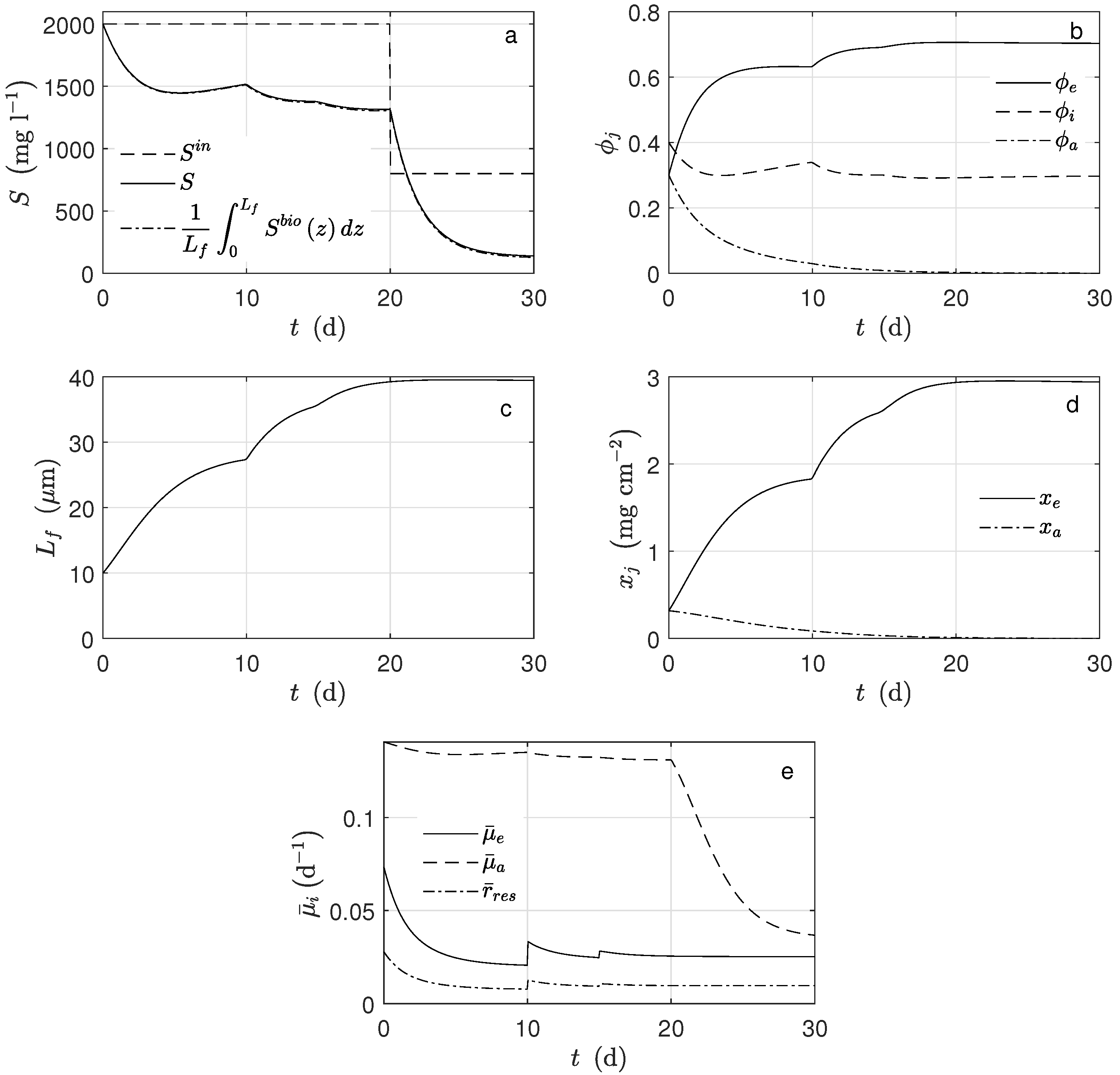
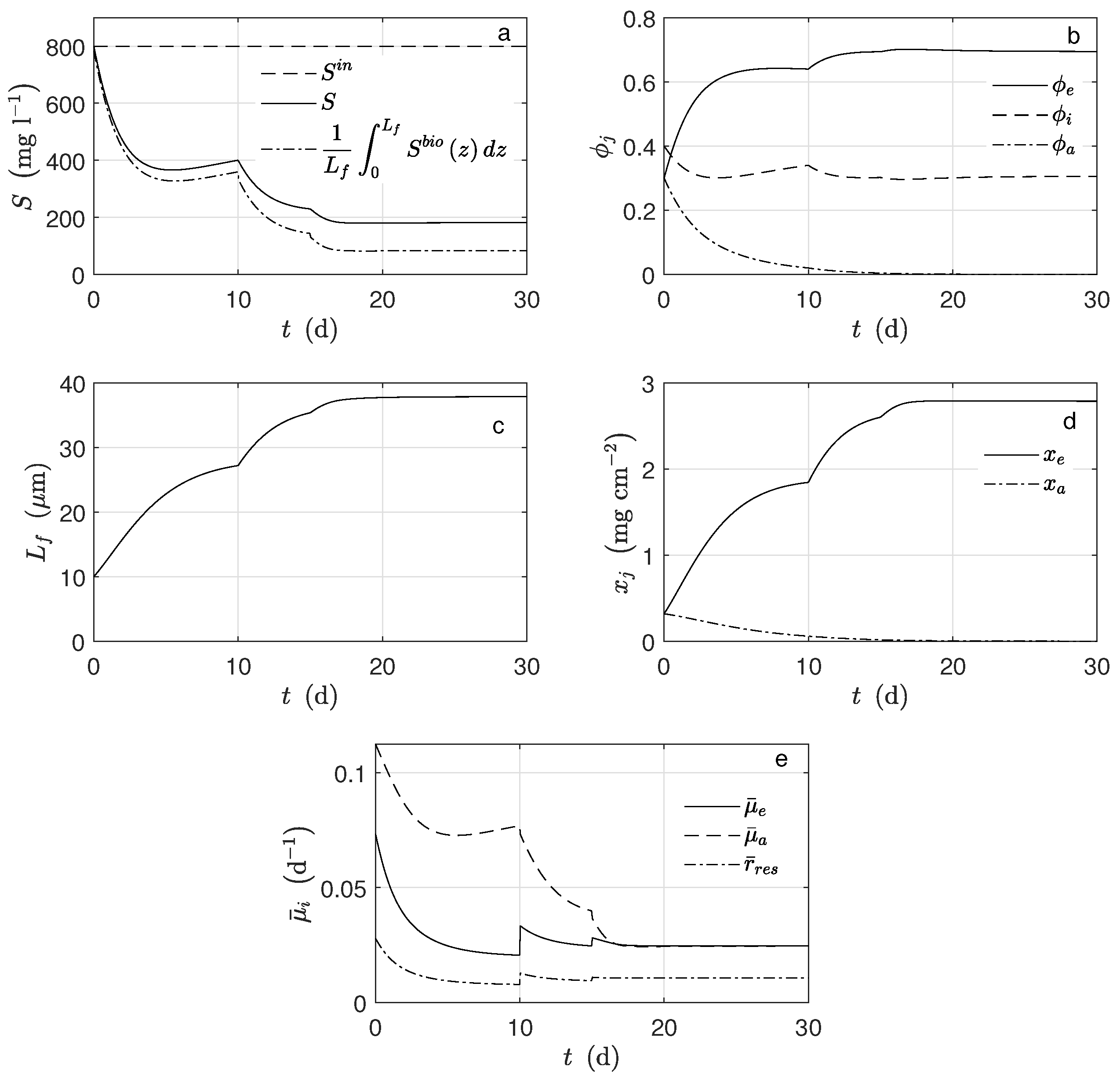
Figure 3 shows the average concentration of substrate inside the biofilm and the concentration in the bulk (
). Notice that both practically overlap. When the substrate concentration at the inlet of the system was perturbed, (
d), the exoelectrogens microorganisms activity was not affected, i.e., the biomass concentration and the produced current remained constant. The primary factor here is that under these conditions, the multiplicative term of the growth kinetic related to the substrate was saturated. It can be proven that 95% of this term was reached when the acetate concentration was 19 mg L
−1. Therefore, the substrate concentration was not a controlling factor for the exoelectrogens microorganisms in the case of this study.
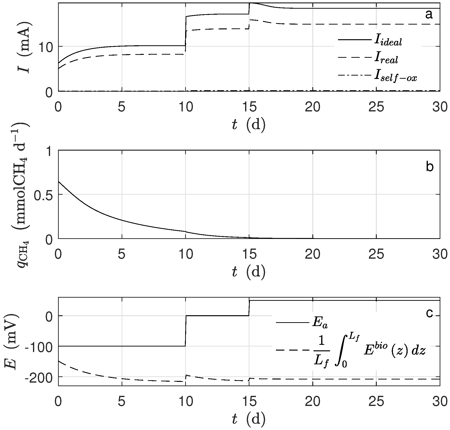
In this case, the kinetic growth rate of the exoelectrogen microorganisms was strongly affected by the potential. It was observed that in every moment, the average potential (
Figure 4c) inside the biofilm was lower than
(mV). Hence, the Nernst–Monod term controlled the growth rate because this term was far from its saturation. It is important to mention that the effects on the biomass concentration (
Figure 3c,d) and the current (
Figure 4a) were evident when the applied potential changes (
Figure 4c). If the potential increased, the exoelectrogens microorganisms transferred the electrons more easily, and their growth rate increased; thus, the biofilm thickness (
Figure 3b) increased.
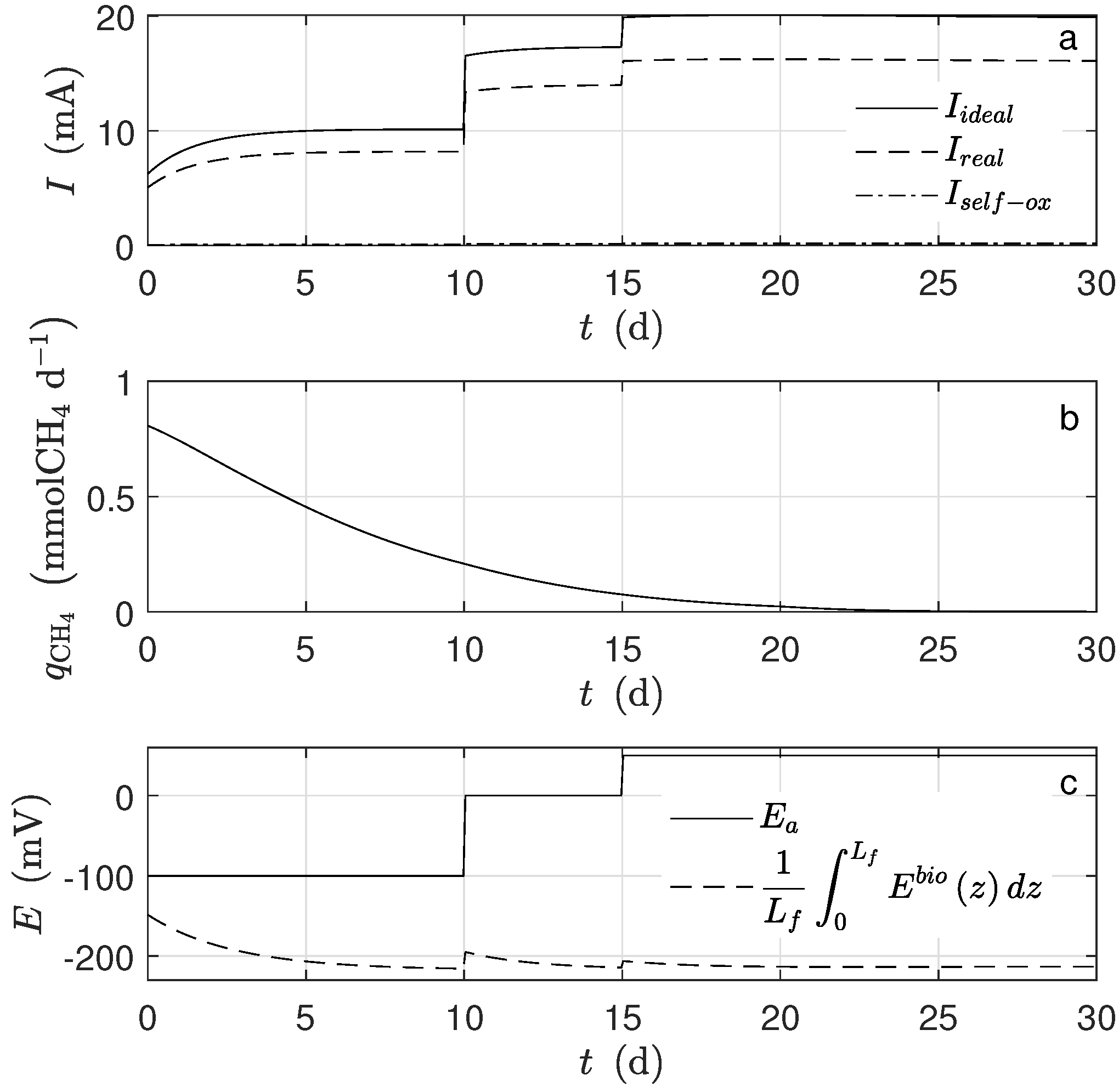
The produced electrons, according to the assumptions, came from two different sources, the metabolized acetate and the self-oxidized biomass, which was too small to be noticed. Moreover, not all the produced electrons went to the electrode. Indeed, some of them were used for the microorganisms’ growth and some others went to a different electron acceptor. The quantity
(
Figure 4a) was calculated under the assumption that all the produced electrons went to the electrode.
For the simulation, equal mass amounts of both microorganism types were assumed for the initial conditions. However, their concentration behaviors were completely different: the amount of exoelectrogens microorganisms increased, and that of the acetoclastic methanogens decreased (
Figure 4d). Under the operational condition for
d, there was no methanogen microorganism activity; thus, there was no methane production (
Figure 4b). The main cause was the big difference between
and
, parameters describing how much substrate is transformed into biomass. According to the assumed values, the exoelectrogens microorganisms produced almost 20 times more biomass per mole of acetate than the methanogens. It can also be observed that the biofilm thickness reached a steady-state, and this happened when the rate of detachment was equal to the biomass production. The inactivation process completely determined the steady-state amount of inert biomass in the biofilm.
4.2. Linear Voltammetry
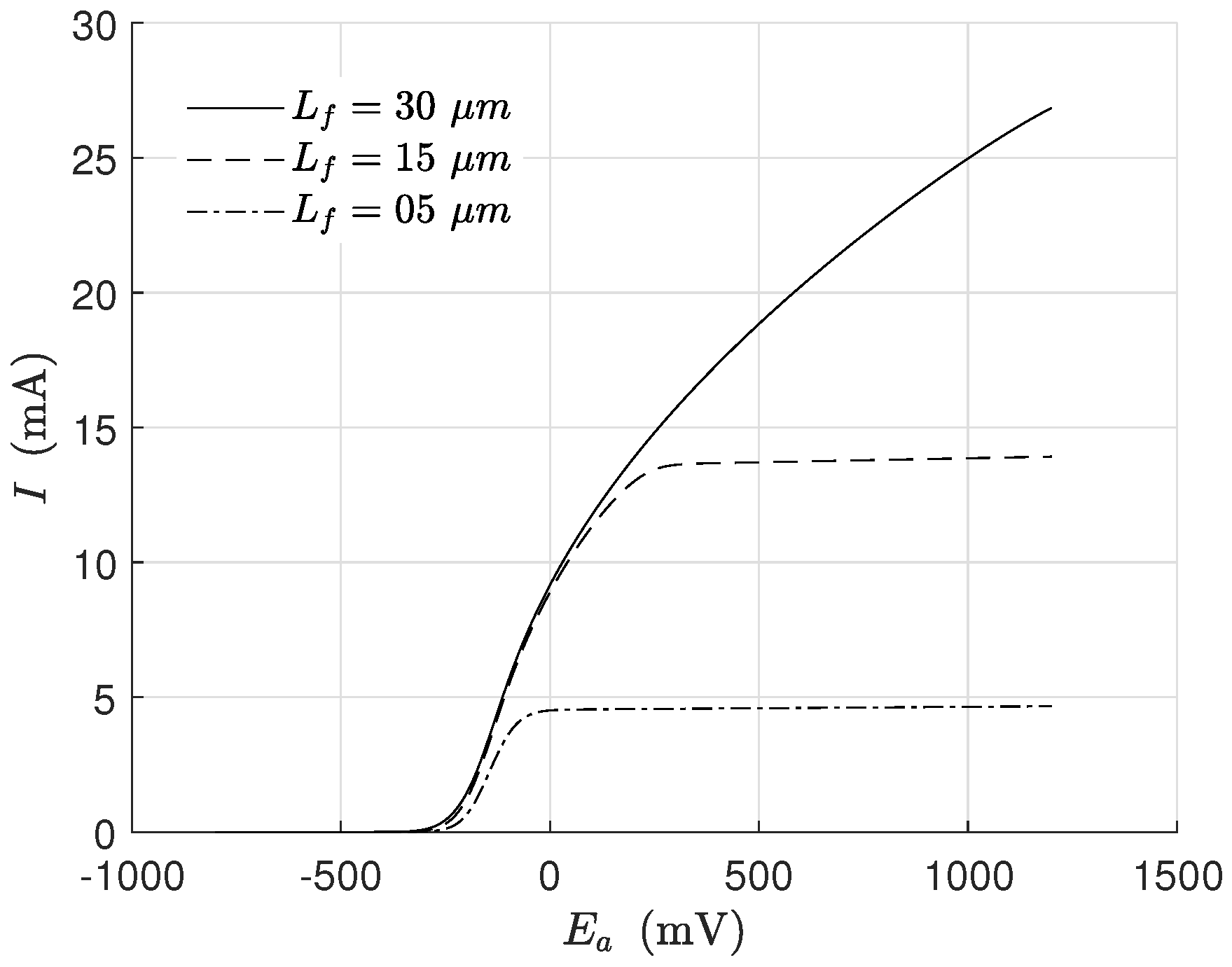
Linear voltammetry is an electrochemical technique reported in many papers that tries to identify the behavior of the exoelectrogen microorganisms under the influence of an applied potential. In
Figure 5 is presented a voltammetry simulation for different biofilm thicknesses. The process consisted of varying the applied potential and keeping the other inputs constant (
Table 1 and
Table 2). The scan was a rapid potential variation (in this case, 40 min) to assure that other changes in biomass concentration did not affect the overall behavior significantly during the voltammetry.
The simulated behavior was completely in line with previous experiments [
26,
30]. It is seen how the current increased for thicker biofilms (due to the more significant biomass concentration). In this simulation, the growth kinetics was affected only by the potential because of the term related to the substrate being saturated.
4.3. Additional Numerical Results
In the following, the case where the kinetics was not saturated is considered. It is important to notice that from a practical point of view, it is convenient to operate in saturation conditions to remove as much substrate as possible. However, in order to explore this nonsaturated scenario, two variables were modified. The first key variable was the inlet substrate concentration at the inlet of the system. In this sense, the inlet substrate concentration was reduced from mg L−1 to mg L−1. The second modified parameter was the diffusion coefficient from cm−1 d−1 to cm−1 d−1.
Figure 6a shows the dynamical behavior of potential inside the biofilm. Notice that the potential drop across the biofilm was significant, and notice as well that the average concentration in the biofilm was smaller than the bulk concentration.
Figure 6a shows the dynamical behavior of substrate concentration inside the biofilm. In this case, the mass diffusion effect was significant at a low inlet concentration. For
d, the concentration decreased from the bulk concentration of 200 mg L
−1 to zero.
Figure 7 shows the dynamical behavior of the reaction rates inside the biofilm. For
d, as the mass diffusion effect was significant, the reactions rates varied significantly. In particular, for
d
(
Figure 7b) and
(
Figure 7c), they were near to zero from
to
.
Figure 8a, shows that there was a significant difference between bulk substrate concentration and substrate average along the biofilm. Under this scenario, the numerical results of biomass fraction, thickness grown, and biomass concentration (see
Figure 8b–d, respectively) were lower than those obtained using a typical set of parameters obtained from the literature. Such a difference was significant for
(see
Figure 8e). As a result, the lower current was obtained (see
Figure 9a).
At a low diffusion coefficient and low substrate concentration at the inlet of the system, the profile of the substrate along the biofilm (
Figure 6b) changed concerning the parameters obtained from the literature (
Figure 1b).

 ,
, 


