Performance Evaluation Using Multivariate Non-Normal Process Capability

Abstract

Process capability indices (PCIs) have always been used to improve the quality of products and services. Traditional PCIs are based on the assumption that the data obtained from the quality characteristic (QC) under consideration are normally distributed. However, most data on manufacturing processes violate this assumption. Furthermore, the products and services of the manufacturing industry usually have more than one QC; these QCs are functionally correlated and, thus, should be evaluated together to evaluate the overall quality of a product. This study investigates and extends the existing multivariate non-normal PCIs. First, a multivariate non-normal PCI model from the literature is modeled and validated. An algorithm to generate non-normal multivariate data with the desired correlations is also modeled. Then, this model is extended using two different approaches that depend on the well-known Box–Cox and Johnson transformations. The skewness reduction is further improved by applying heuristics algorithms. These two approaches outperform the investigated model from the literature because they can provide more precise results regardless of the skewness type. The comparison is made based on the generated data and a case study from the literature.

1. Introduction

Variability in the outputs of manufacturing processes has been studied for decades. It is investigated using many techniques, such as the design of experiments, and statistical process controls, especially with the help of process capability analysis [1]. Advances in industrial systems have required process engineers to widely analyze and control each element in their processes [2]. Using process capability analysis, we can evaluate manufacturing processes and use this information to improve the capabilities of the considered processes to meet the desired specifications.

It is an established fact that most manufacturing products have more than one quality characteristic (QC). Moreover, these QCs are functionally correlated, implying that they should be considered together. Consequently, the product quality evaluation process becomes more complex as the number of QCs increases, leading to increased interest in finding capability indices that can address multivariate non-normal process capabilities. For example, Wang [3] performs a process capability analysis for a real-world product with seven QCs.

Multivariate process capability analysis is a common topic of interest in the literature. Taam et al. [4] propose the first multivariate capability index using the concepts of process regions (PRs) and specification regions (SRs). Chen [5] presents the first multivariate Cp that uses the proportion of non-conformance (PNC). Shahriari et al. [6] evaluate the performance of multivariate QCs using process capability analysis. Braun [7] investigates the shapes of the process PRs and SRs to define a new process capability index (PCI). Castagliola et al. [8] study bivariate process capabilities and derive two indices based on the PNC. Bothe [9] establishes a method for estimating a multivariate $C_{pk}$ index. Wang et al. [10] define a new index from $C_p$ and $C_{pk}$ based on a principal component analysis (PCA) decomposition.

The literature includes many other studies in the field of multivariate capability analysis [3,11,12,13,14,15,16,17,18,19,20,21,22,23,24,25,26,27,28,29,30,31,32,33,34,35,36]. PCA was first used in process capability analysis by Wang and Chen [37]. Chen [5] presents one of these multivariate PCIs by establishing a comparison between the original PR and SR. Although he compares the PR to the SR, Chen does not consider the position of the PR within the SR in his investigation. Das and Dwivedi [28] use the g and h multivariate PCI for non-normal data. Their proposed PCI has been compared to other PCIs in the literature, and it performs well. However, the process of finding this PCI requires some complex computations. Ciupke [22] proposes a multivariate PCI that can be used for normal and non-normal QCs. He suggests the use of one-sided models to determine the PR, which is compared with SR in the evaluation of multivariate non-normal processes. Pan et al. [20] extend the work of Pan and Lee [32] to propose a multivariate non-normal PCI. They estimate the original probability density function using a weighted standard deviation. Castagliola [38] define the traditional PCIs (Cp, and Cpk) based on the PNC.

Many previous studies have been conducted on PCIs in this group. However, most of these studies deal with multivariate normal data [39,40]. Nevertheless, some attempts have been made to extend the use of the PNC to non-normal data. Abbasi and Niaki [41] use the concept of the PNC to develop a multivariate non-normal PCI. They use the root transformation method to normalize non-normal data and then use Monte Carlo simulation to estimate the PNC. Ahmad et al. [33] investigate multivariate non-normal process capability analysis based on the PNC. They reduce the dimension of the multivariate QCs using the covariance distance (CD). Many studies in the literature consider non-normal PCIs [8,11,42,43,44,45,46,47,48,49,50]. Additionally, a few studies focus on multivariate non-normal process capabilities. The number of such studies increases yearly [3,11,25,27,44,51,52,53,54,55,56,57,58,59].

Most of existing multivariate PCIs are based on normality theory and treat multivariate QCs as normal data. However, most real-world data on QCs do not follow a normal distribution. Moreover, the proposed non-normal multivariate PCIs in the literature still have many limitations. These limitations relate to the following issues:

• Most of the proposed multivariate PCIs depend on the normality assumption;
• Some can only be used in specific circumstances [41];
• Some proposed PCIs can only deal with two QCs [60];
• Some multivariate PCIs are limited to a specific distribution [60];
• The complexity of the statistical calculations can limit implementations [20].

Consequently, the provision of a robust multivariate PCI is still a great research opportunity.

The objective of this study is to provide a multivariate non-normal capability index that takes into account correlations between QCs, regardless of data skewness type. Although, Abbasi and Niaki [41] propose a methodology for estimating PCIs for multivariate non-normal processes for right-skewed data, it fails to reduce the skewness of left-skewed data. However, in practice, many multivariate manufacturing processes contain positive (right-sided) and negative (left-sided) skewness (Figure 1).

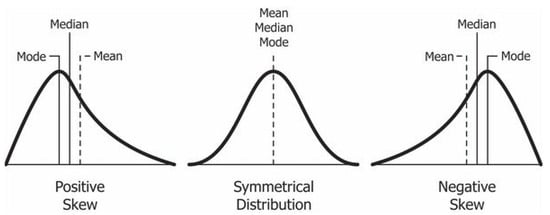
Figure 1. Types of data skewness.

Owing to the limitations of the proposed methods for estimating multivariate non-normal process capabilities in the literature [41], carrying out different transformations is an important research opportunity. These transformation techniques, such as the Box–Cox and Johnson transformations [61,62], can be used, and their performances can be evaluated.

The rest of this article is organized as follows. Section 2 provides a theoretical background on process capability analysis. The methodology is presented in Section 3. Section 4 presents and discusses the results revealed by applying the implemented methodology. Finally, Section 5 concludes the study and suggests some directions for future research.

2. Theoretical Background

It is worth noting that process monitoring precedes the use of process capabilities. The stability of a process is usually tested using quality control charts. Montgomery [63] provides a useful presentation of statistical process controls.

After the stability of a process is determined, its capabilities can be analyzed using different tools, such as histograms, descriptive statistics, and skewness [63]. The most important method in a capability analysis is called the process capability index (PCI). A PCI is a unitless measure that quantifies the relation between the actual performance of a process and its specified requirements. PCIs are proposed to predict the proportion of products that are not expected to meet a given set of specifications. Generally, the higher the PCI value, the lower the proportion of non-conformance (PNC). Juran and Frank [64] propose a PCI for process capability assessment with the assumption $C_p$, as follows:

$$C_p=\frac{USL-LSL}{6\sigma },$$

(1)

where USL is the upper specification limit of the process, LSL is the lower specification limit, and $\sigma$ is the standard deviation of the process data. Moreover, if the process data follow a normal distribution $N\left(\mu ,{\sigma }^2\right)$, then we can say that the process is centered at its nominal mean. If its actual mean is defined by

$$m=\frac{USL+LSL}{2},$$

(2)

that is, $E\left(x\right)=\mu =m$, then the process is considered capable if $C_p\ge 1$. then we can say that the process is centered at its nominal mean. If its actual mean is defined by.

Such a process results in a percent of non-conforming items of at most 0.27%, that is, 2700 nonconforming items per million items produced in a production process, which is small [65].

In most cases, the process mean does not equal the nominal mean, but rather, is shifted somewhat. Process capability assessment using the ${\mathrm{C}}_{\mathrm{p}}$ index does not take into account this shift. Thus, another PCI, called $C_{pk}$, was proposed by Kane [66]. This PCI depends on the minimum assessments of the upper and lower capability indexes $(C_{pu}, \mathrm{and} C_{pl})$.

$$C_{pu}\left(Upper{C}_p\right)=\frac{USL-\mu }{3\sigma },$$

(3)

$$C_{pl}\left(Lower{C}_p\right)=\frac{\mu -LSL}{3\sigma },$$

(4)

where μ and σ are the mean and standard deviation, respectively, of the in-control process.

$$C_{pk}=min\{\begin{array}{c}\frac{USL-\mu }{3\sigma }\\ \frac{\mu -LSL}{3\sigma }\end{array}$$

(5)

It is worth noting that $C_p$ is linked to the PNC [67]. Suppose that the QC, X, is normally distributed. Then, the PNC is expressed as:

$$\begin{gathered} PNC=P\left(X>USL\right)+P\left(X<LSL\right)=\left(1-p\left(X<USL\right)\right)+P\left(X<LSL\right) \\ =\left(1-\varphi \left(\frac{USL-\mu }{\sigma }\right)\right)+\varphi \left(\frac{LSL-\mu }{\sigma }\right) \end{gathered}$$

(6)

If $\mu$ is replaced with the nominal mean $\left(\left(USL+LSL\right)/2\right)$, as stated in Equation (2), the PNC is calculated as:

$$PNC=2\varphi \left(-3C_p\right),$$

(7)

where $\varphi \left(x\right)$ is the cumulative distribution function of the unit Gaussian.

The PNC can also be expressed as the number of defects in terms of parts per million (PPM). Table 1 shows the number of defects in PPM terms for some $C_p$ values. The $C_p$ value can also be used to specify the sigma level of a process. For example, if $C_p=2$, the process is at the six sigma level, and if $C_p=1$, the process is working at the three sigma level [3].

Table 1. Minimum expected proportion of non-conformances (PNCs).

${\mathit{C}}_{\mathit{p}}$	2	5/3 = 1.67	4/3 = 1.33	1	2/3 = 0.667	1/3 = 0.33
PPM	0.002	0.57	63	2700	45,500	317,300
ppm = parts per million

Process capability analysis is mainly based on probability theory. Consequently, the PCI should be fitted to a specific probability distribution that can be used to estimate its index given its variation [8]. The traditional PCIs, such as $C_p$ and $C_{pk}$, are used when the QCs are normally distributed. However, in practice, quality specialists should verify the normality assumptions before conducting performance analysis using the traditional PCIs. Clements [43] developed one of the most famous PCIs that can be used for univariate non-normal QCs.

$$C_p\left(q\right)=\frac{USL-LSL}{{\chi }_{0.99865}-{\chi }_{0.00135}}$$

(8)

This PCI uses non-normal quantiles instead of $6\sigma \mathrm{and}\mu$, which were used in Equation (1). Here, qα represents the quantiles of a distribution in the Pearson family for the specified α values.

Multivariate process capability analysis is the process of quantifying multiple QCs of a product using a single PCI. This index can be used to evaluate the quality of a product, as well as the capabilities of a process. Many studies in the literature aim to provide a practical measure of multivariate non-normal process capabilities. This study focuses on providing a multivariate non-normal capability index that takes into account correlations between QCs.

Generally, a multivariate PCI is a single number that can evaluate the quality of a considered product using multiple QCs for that product. Different methods can be used to determine a multivariate PCI, such as:

• Computing the ratio of the tolerance limits to the process variation;
• Using the PNC for the relevant products;
• Exploring global multivariate quality control methods.

$$C_p=\frac{{\mathsf{\phi }}^{-1}\left(0.5+0.5\left(1-\mathrm{PNC}\right)\right)}{3}$$

(9)

3. Research Methodology

This study investigates a multivariate PCI for both right- and left-skewed data. First, the root transformation method, which is proposed in the literature [41], is validated and adopted for the same non-normal data as in the literature. Then, the performances of the Box–Cox and Johnson transformations for PCI calculations are investigated. The study applies two algorithms for Box–Cox and Johnson transformations to investigate multivariate PCIs for non-normal data. Statistical and heuristic methods are used to identify the best parameters for the transformation techniques. Figure 2 presents a flow chart for the applied methodology.

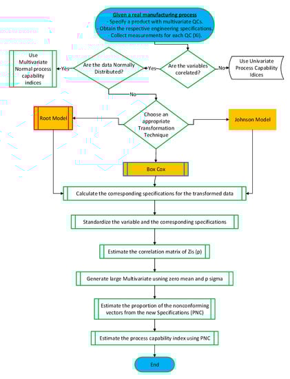
Figure 2. Research methodology.

The methodology in this study consists of several steps that lead to an estimated PCI for multivariate non-normal data as shown in Table 2. The methodology suggests three types of transformation techniques to normalize the data. Furthermore, the specification limits are transformed using either the same techniques or prediction techniques. Then, the transformed data are standardized ${\mathrm{as}\mathrm{Z}}_{\mathrm{i}}=\frac{{\mathrm{Y}}_{\mathrm{i}}-\widehat{{\mathsf{\mu }}_{{\mathrm{Y}}_{\mathrm{i}}}}}{\widehat{{\mathsf{\sigma }}_{{\mathrm{Y}}_{\mathrm{i}}}}};\mathrm{i}=1,2,\dots ,\mathrm{p}$, where Y_i represents the transformed data and p is the number of QCs. Then, the correlation matrix of ${\mathrm{Z}}_{\mathrm{i}}$, denoted by $\widehat{{\mathsf{\Sigma }}_{\mathrm{z}}}$, is estimated in the next step in which a large sample from a multivariate normal distribution with mean zero and covariance $\widehat{{\mathsf{\Sigma }}_{\mathrm{z}}}$z is generated. Then, based on the transformed specification limits, the PNC of the generated sample is estimated. Finally, Equation (10) is used to estimate the process PCI:

$$C_p=\frac{{\phi }^{-1}\left(0.5+0.5\left(1-PNC\right)\right)}{3}$$

(10)

Table 2. Research methodology steps.

Steps	Descriptions	Comments
Step 1	Collect the sample (X), by specifying the process, the number of its QCs (p), and the sample size (n).	Since X consists of p of QCs, and p ≥ 2. Each QC consists of n sample size.
Step 2	Compute parameters for each transformation method.	Use algorithms in Figure 3, Figure 4 and Figure 5, to compute the best parameters for Root, Box–Cox, and Johnson transformations, respectively.
Step 3	Compute transformed variable $({\mathrm{Y}}_{\mathrm{i}}$) with the corresponding transformation function for each method.	${\mathrm{Y}}_{\mathrm{i}}={\mathrm{Y}}_{\mathrm{i}}\left({\mathrm{X}}_{\mathrm{i}}\right);\mathrm{i}=1,2,\dots ,\mathrm{p}$.
Step 4	Estimate the mean and the standard deviation of the transformed variable ${\mathrm{Y}}_{\mathrm{i}}$, say $\widehat{{\mathsf{\mu }}_{{\mathrm{Y}}_{\mathrm{i}}}}\mathrm{and}\widehat{{\mathsf{\sigma }}_{{\mathrm{Y}}_{\mathrm{i}}}}$.	$\widehat{{\mathsf{\mu }}_{{\mathrm{Y}}_{\mathrm{i}}}}=\mathrm{E}\left({\mathrm{Y}}_{\mathrm{i}}\right),\widehat{{\mathsf{\sigma }}_{{\mathrm{Y}}_{\mathrm{i}}}}=\sqrt{\widehat{\mathrm{Var}}(}{\mathrm{Y}}_{\mathrm{i}})$.
Step 5	Compute the standardized variable ${\mathrm{Y}}_{\mathrm{i}}$ as ${\mathrm{Z}}_{\mathrm{i}}=\frac{{\mathrm{Y}}_{\mathrm{i}}-\widehat{{\mathsf{\mu }}_{{\mathrm{Y}}_{\mathrm{i}}}}}{\widehat{{\mathsf{\sigma }}_{{\mathrm{Y}}_{\mathrm{i}}}}};\mathrm{i}=1,2,\dots ,\mathrm{p}$.	$\mathrm{Z}=\left[\frac{{\mathrm{Y}}_1-\widehat{{\mathsf{\mu }}_{{\mathrm{Y}}_1}}}{\widehat{{\mathsf{\sigma }}_{{\mathrm{Y}}_1}}}\frac{{\mathrm{Y}}_2-\widehat{{\mathsf{\mu }}_{{\mathrm{Y}}_2}}}{\widehat{{\mathsf{\sigma }}_{{\mathrm{Y}}_2}}}\dots \frac{{\mathrm{Y}}_{\mathrm{p}}-\widehat{{\mathsf{\mu }}_{{\mathrm{Y}}_{\mathrm{p}}}}}{\widehat{{\mathsf{\sigma }}_{{\mathrm{Y}}_{\mathrm{p}}}}}\right]$.
Step 6	Estimate the correlation matrix of Z, say $\widehat{{\mathsf{\Sigma }}_{\mathrm{z}}}$.
Step 7	Transform, standardized the specifications limits by the same parameters of steps 3 and 5.	Compute ${\mathrm{USL}}_{\mathrm{z}}{\mathrm{and}\mathrm{LSL}}_{\mathrm{z}}$.
Step 8	Generate large (N) sample vectors from multivariate normal with mean zero and covariance $\widehat{{\mathsf{\Sigma }}_{\mathrm{z}}}$.	$\mathrm{N}=\mathrm{Total}\#\mathrm{of}\mathrm{generated}\mathrm{vectors}$.
Step 9	Estimate PNC.	$\mathrm{NNC}=\#\mathrm{of}\mathrm{vectors}\mathrm{out}\mathrm{of}\mathrm{USL}\&\mathrm{LSL}$ $\mathrm{PNC}=\frac{\mathrm{NNC}}{\mathrm{N}}$.
Step 10	Estimate PCI using PNC.	${\mathrm{C}}_{\mathrm{p}}$=$\frac{{\mathsf{\phi }}^{-1}\left(0.5+0.5\left(1-\mathrm{PNC}\right)\right)}{3}$.

Aside from the model taken from prior studies, the models used follow similar procedures for finding the PCI in the case of multivariate non-normal QCs. However, the three models differ from each other in their skewness reduction methods and in estimating the new specification limits for transformed data. In the next sections, each model is discussed separately.

3.1. Root Transformation

Root transformation, which was proposed by Abbasi and Niaki [41], consists of three main stages. First, the skewness of the marginal probability distributions of the variables is diminished using a root transformation technique.

• A Monte Carlo simulation method is employed to estimate the process PNC;
• The relationship between the PNC and PCI is found;
• The PCI is estimated using the PNC.

Although this method mentions two-sided specifications, it supposes that the marginal distributions are right-skewed for most non-normal processes, and, thus, only the USL must be defined.

The root transformation technique searches for a proper root (r) of the right-skewed non-normal data such that if the data were raised to the power r $\left({\mathrm{X}}^{\mathrm{r}}\right)$, the skewness in the distribution of the transformed data would be almost zero. The bisection method is employed to find the appropriate value of r. This method is based on the point at which a function changes sign when it passes through zero. By evaluating a function in the middle of an interval and replacing whichever limit has the same sign, the bisection method can halve the size of the interval in different iterations to eventually find the root. For example, to find the root of $\mathrm{f}\left(\mathrm{x}\right)=0$ in the interval of $\left(\mathrm{a}0,\mathrm{b}0\right)$, where $\mathrm{f}\left({\mathrm{a}}_0\right)\mathrm{f}\left({\mathrm{b}}_0\right)<0$, a tolerance $\mathsf{\epsilon }$ is chosen, and the algorithm in Figure 3 is then applied:

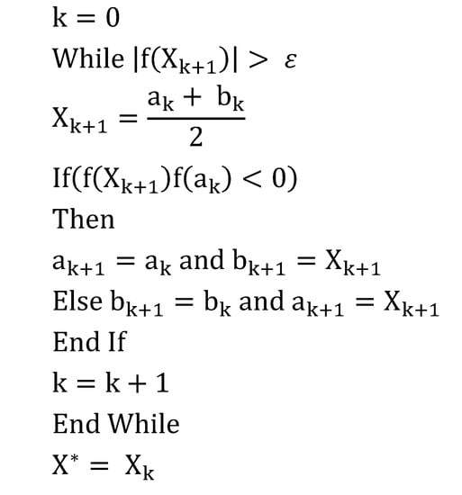
Figure 3. Root transformation algorithm.

To estimate a PCI for multivariate non-normal processes, the root transformation technique can first be applied to diminish the skewness in the marginal distributions of the ${\mathrm{X}}_{\mathrm{i}}’\mathrm{s}$ until the skewness is less than the tolerance or until a specific number of iterations has been performed. The specification limits of the original variables are transformed in the same manner, that is, by raising each specification limit to the power given by the root obtained for its corresponding variable and then standardizing it in the same way as its corresponding variable is standardized. Through this procedure, a new specification limit is obtained for each ${\mathrm{Z}}_{\mathrm{i}}$. As an example, assume that the upper specification limit of the $i\mathrm{th}$ original QC (${\mathrm{X}}_{\mathrm{i}}$) is ${\mathrm{USL}}_{\mathrm{xi}}$. Then, the upper specification limit of the $i\mathrm{th}$ standardized-transformed variable (${\mathrm{Z}}_{\mathrm{i}}$) is ${\mathrm{USL}}_{\mathrm{zi}}$ which is calculated using Equation (11).

$$US{L}_{z_i}=\frac{{(US{L}_{x_i})}^{r_i}-\widehat{{\mu }_{Y_i}}}{\widehat{{\sigma }_{Y_i}}}$$

(11)

Here, $\widehat{{\mathsf{\mu }}_{{\mathrm{Y}}_{\mathrm{i}}}}$ and $\widehat{{\mathsf{\sigma }}_{{\mathrm{Y}}_{\mathrm{i}}}}$ are the estimated mean and standard deviation of the $i\mathrm{th}$ transformed variable, and ${\mathrm{r}}_{\mathrm{i}}$ is the root obtained for the $i\mathrm{th}$ original variable such that the skewness of ${\mathrm{X}}_{\mathrm{i}}^{{\mathrm{r}}_{\mathrm{i}}}$ is almost zero. If both the upper and lower specification limits are given, the equations for the specification limits change as follows:

$$LS{L}_{z_i}=\frac{{(LS{L}_{x_i})}^{r_i}-\widehat{{\mu }_{Y_i}}}{\widehat{{\sigma }_{Y_i}}}andUS{L}_{z_i}=\frac{{(US{L}_{x_i})}^{r_i}-\widehat{{\mu }_{Y_i}}}{\widehat{{\sigma }_{Y_i}}}$$

(12)

3.2. Box–Cox Transformation

In this study, we extend the research in the literature by considering the estimation of λ using a different methodology. Specifically, we use a searching algorithm which finds the argument of minimum skewness over a pre-specified interval for the candidate λ values. Furthermore, this extended method and that of Abbasi and Niaki [41] are illustrated using real-world datasets with seven QCs that include right- and left-skewed data.

The Box–Cox power transformation [61] on observations ${\mathrm{y}}_{\mathrm{i}}\left(\mathrm{i}=1,2,\dots ,\mathrm{n}\right)$ is given by

$${y_i}^{\left(\lambda \right)}=\{\begin{array}{cc}\frac{y_i{}^{\lambda }-1}{\lambda },& if\lambda \ne 0,\\ log{y}_i, & if \lambda =0\end{array}$$

(13)

where λ is an unknown power transformation parameter and n is the sample size.

Depending on the Box–Cox transformation, a heuristic algorithm is used in this analysis to obtain the best value of λ to effectively reduce the absolute skewness value. The algorithm is provided in Figure 4. This algorithm starts by ensuring that each element of the dataset is positive. Otherwise, a small constant is added to all observations to shift the dataset to positive values, as originally proposed by Box and Cox [61]. Then, a sequence of candidate λ values is selected using a fairly precise increment, such as 0.1, 0.02, and so on, in a specified interval. The Box–Cox power transformation given by Equation (13) is applied using all the candidate λ values to obtain as many transformed samples as the number of λ values. The skewness of each of these transformed samples is checked, and the λ value that corresponds to the minimum skewness is selected.

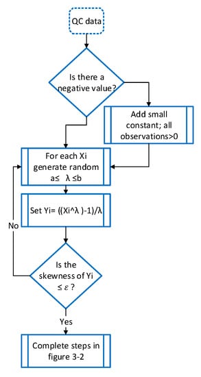
Figure 4. Algorithm for determining the best Box–Cox parameter.

3.3. Johnson Transformation

A Johnson transformation is used to estimate the PCI for multivariate non-normal data. The search for its optimal parameters is conducted in two stages. Initially, the appropriate type of Johnson family distribution for the QC data is determined using the percentile method. Then, the parameters of the selected Johnson distribution are calculated; these parameters serve as an initial solution in the next stage. Typically, the parameters estimated using the percentile method do not work well for skewness reduction. However, they can be used as an initial solution because the optimal parameters are usually close to the parameters estimated using the percentile method. The second stage is called the heuristic method. In this stage, small increments are added to and subtracted from the parameters estimated in the initial solution in a specific number of iterations. Those with the least skewness are the optimal parameters.

3.3.1. Percentile Method

The crucial process in the given non-normal data is to fit to the right family of Johnson distribution. Given any of the transformations described in Table 3, choose a specific value z > 0 from the standard normal variables. Next, consider four points of $\pm$z and $\pm$3z, which establishes three equal intervals. Let $x_{3z}, x_z, x_{-z}, x_{-3z}$ be the values corresponding to $3z, z, -z,\mathrm{and} -3z$ under the Johnson transformation. The following steps are used to determine the appropriate type of Johnson transformation:

Table 3. Summary of Johnson transformation systems [62].

Johnson System	Bounded System (SB)	Lognormal System (SL)	Unbounded System (SU)
Johnson Curve	${\tau }_3\left(x,\epsilon ,\lambda \right)=\mathit{log}\left(\frac{x-\epsilon }{\lambda +\epsilon -x}\right)$	${\tau }_1\left(x,\epsilon ,\lambda \right)=\mathit{log}\left(\frac{x-\epsilon }{\lambda }\right)$	${\tau }_2\left(x,\epsilon ,\lambda \right)= {\mathit{sinh}}^{-1}\left(\frac{x-\epsilon }{\lambda }\right)$
Normal Transformation	$z=\gamma +\eta \mathit{ln}\left(\frac{x-\epsilon }{\lambda +\epsilon -x}\right)$	$z=\gamma +\eta \mathit{ln}(x-\epsilon )$	$z=\gamma +\eta {\mathit{sinh}}^{-1}\left(\frac{x-\epsilon }{\lambda }\right)$
Parameter Constraints	$\eta , \lambda >0$ $-\infty <\gamma <\infty$	$\eta >0$ $-\infty <\gamma <\infty$ $-\infty <\epsilon <\infty$	$\eta , \lambda >0$ $-\infty <\gamma <\infty$ $-\infty <\epsilon <\infty$
X Constraint	$\epsilon \le x\le \epsilon + \lambda$	x≥$\epsilon$	$-\infty <x<\infty$

• Step 1: Choose an appropriate value of z;
• Step 2: From the normal standard table of normal distribution, obtain the probability distribution $p_{-sz},p_{-z},p_z,\mathrm{and}{p}_{sz}\mathrm{for}(-sz,-z,z,sz)$;
• Step 3: Find the corresponding quantiles $x_{-sz},x_{-z},x_z,\mathrm{and}{x}_{sz}$ in the sample data;
• Step 4: Let $m=x_{sz}-x_z,n=x_{-z}-x_{-sz},p=x_z{x}_{-z}$;
• Step 5: Define the quantile ratio $(\mathrm{QR}=\mathrm{m}*\mathrm{nL}/p^2)$;
• Step 6: Select the appropriate Johnson system as follows:

$$Johnsonsystemtype=\{\begin{array}{c}{S}_B, QR<1\\ S_L, QR=1\\ S_U, QR>1\end{array}.$$

In step 1, a value of z > 0 is chosen. This choice should be motivated by the number of data points. In general, for moderate-sized datasets, a value of z less than 1.0 is chosen because a z of 1.0 or higher makes it difficult to estimate the percentile points corresponding to +3z. A more typical choice is using a value of z near 0.5, such as z = 0.524. This choice dictates the use of 3z = 1.572, and these two points require estimating the 70th and 94.2th percentiles. However, the larger the number of observations is, the larger the value of z that can be selected. This analysis subsequently shows that z and the estimated p, m, and n can be used to estimate the distribution parameters. Thus, the choice of z can be motivated by seeking a value which assumes a close match to the data and empirical distribution in the areas of greatest interest. Then, a table of areas for the normal distribution is used to determine the percentages $p_{\xi }$ corresponding to $\xi =3z, z, -z, \mathrm{and} -3$. For example, if z = 0.2, then $P_{0.2}$ = 0.5793. For each such, the percentile $x^{\left(\mathrm{i}\right)}$ corresponding to $p_{\xi }$ is obtained from the data using the relationship $\left(i - 1/2\right)/n = p_{\xi }$ and setting $x_{\xi }$= $x^{\left(i\right)}.$ Here, n is the number of data points. Thus, $x_{\xi }$ is the $i\mathrm{th}$ ordered observation, where $i = n{p}_{\xi }+ 1/2$. Because i is not generally an integer, it may be necessary to interpolate. From the values obtained in the previous step, the sample values of m, n, and p can be computed, and the criteria in step 6 can be used to select the appropriate Johnson system.

Johnson $S_U$ Distribution

The formula for transforming non-normal data using the Johnson $S_U$ Distribution is as follows:

$$z=\gamma +\eta {\mathit{sinh}}^{-1}\left(\frac{x-\epsilon }{\lambda }\right)$$

The values of the parameters are presented in such a way as to emphasize their dependence on the ratios m/p and n/p. The parameter estimates for the Johnson $S_U$ distribution are as follows.

$$\eta =\frac{2z}{{\cosh }^{-1}\left[\frac{1}{2}\left(\frac{m}{p}+\frac{n}{p}\right)\right]};\left(\eta >0\right)$$

$$\gamma ={\mathsf{\eta }\sin \mathrm{h}}^{-1}\left[\frac{\frac{n}{p}-\frac{m}{p}}{2{\left(\frac{m}{p}\frac{n}{p}-1\right)}^{\frac{1}{2}}}\right];$$

$$\lambda =\frac{2p{\left(\frac{m}{p}\frac{n}{p}-1\right)}^{\frac{1}{2}}}{\left(\frac{m}{p}+\frac{n}{p}-2\right){\left(\frac{m}{p}+\frac{n}{p}+2\right)}^{\frac{1}{2}}};\left(\lambda >0\right)$$

$$ϵ=\frac{x_z+x_{-z}}{2}+\frac{p\left(\frac{n}{p}-\frac{m}{p}\right)}{2\left(\frac{m}{p}+\frac{n}{p}-2\right)}$$

Johnson $S_B$ Distribution

$$z=\gamma +\eta \mathit{ln}\left(\frac{x-ϵ}{\lambda +ϵ-x}\right)$$

The solutions for the $S_B$ parameters depend on the ratios p/m and p/n (as opposed to m/p and n/p in the case of the $S_U$ parameters). The parameter estimates for the Johnson $S_B$ distribution are as follows.

$$\eta =\frac{z}{{\cosh }^{-1}\left[\frac{1}{2}{\left(\left(1+\frac{p}{m}\right)+\left(1+\frac{p}{n}\right)\right)}^{\frac{1}{2}}\right]};\left(\eta >0\right)$$

$$\gamma ={\mathsf{\eta }\sin \mathrm{h}}^{-1}\left[\frac{\left(\frac{p}{n}-\frac{p}{m}\right){\left[\left(1+\frac{p}{m}\right)\left(1+\frac{p}{n}\right)-4\right]}^{\frac{1}{2}}}{2\left(\frac{p}{m}\frac{p}{n}-1\right)}\right];$$

$$\lambda =\frac{p{\left[{\left(\left(1+\frac{p}{m}\right)\left(1+\frac{p}{n}\right)\right)}^2-4\right]}^{\frac{1}{2}}}{\frac{p}{m}\frac{p}{n}-1};\left(\lambda >0\right)$$

$$ϵ=\frac{x_z+x_{-z}}{2}-\frac{\lambda }{2}+\frac{p\left(\frac{p}{n}-\frac{p}{m}\right)}{2\left(\frac{p}{m}\frac{p}{n}-1\right)}$$

Johnson $S_L$ Distribution (lognormal)

$$z=\gamma +\eta \mathit{ln}\left(x-ϵ\right)$$

The parameter estimates for the Johnson $S_L$ distribution are as follows.

$$\eta =\frac{2z}{ln\left(\frac{m}{p}\right)}$$

$$\gamma =\eta ln\left[\frac{\frac{m}{p}-1}{p{\left(\frac{m}{p}\right)}^{\frac{1}{2}}}\right]$$

$$ϵ=\frac{x_z+x_{-z}}{2}+\frac{p}{2}\frac{\frac{m}{p}+1}{\frac{m}{p}-1}$$

3.3.2. Heuristic Method

In the Johnson transformation, the closeness of the skewness value to zero is a function of the parameter selection. When applying the Johnson family formulas described above, it can be difficult to vary the parameters to achieve zero skewness in the transformed data because the Johnson transformation has four parameters and the trivial solution is time-consuming. Thus, Johnson transformation parameter selection is a complex problem and requires heuristic solutions. Here, we can use an iteration algorithm to search for the best Johnson transformation parameters that bring skewness closest to zero. The implemented algorithm is presented in Figure 5. This algorithm should specify a specific number of iterations to perform. Then, to speed up the algorithm, the percentile method discussed previously is used to provide an initial solution. Next, the initial parameters are subjected to the addition and subtraction process, and the skewness is evaluated with each addition and subtraction. Finally, the algorithm chooses the parameters with the least absolute value of skewness.

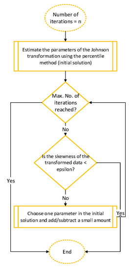
Figure 5. Algorithm for identifying the best Johnson parameters.

3.4. Application and Comparative Examples

The most important step is presenting applications of these methods and a set of comparisons. To do that, two examples from the literature with known PNCs are presented in this section. The first example is discussed and its statistical properties are shown by Abbasi and Niaki [41] (Case 1) without presenting the data, and the second example is presented as a real case study by Wang [3] (Case 2). These two examples are discussed in the next sections.

3.4.1. Case 1

This example includes three distributions and four samples. Each sample is generated with four different sample sizes, as shown in Table 4. The non-normal distributions are the gamma, beta, and Weibull distributions, and the sample sizes are n = 50, 100, 500, and 1000. The USL is also presented for each variable. The shape and scale parameters are denoted by $\beta$, respectively. Additionally, the correlation matrix is presented for each sample. Finally, the actual PCI, $C_p$, is shown in the last column for each sample.

Table 4. Parameters of case 1 [41].

Distribution	n	USL	$\mathit{\alpha }$	$\mathit{\beta }$	Correlation	Actual
gamma	50					0.89
	100	13	1	2	1, 0.49
	500	26	2	3	0.49, 1
	1000
gamma	50	130	5	7	1, −0.37, 0.58	1.18
	100	58	6	3	−0.37, 1, −0.28
	500	150	2	8	0.58, −0.28, 1
	1000
Beta	50					1.12
	100	1	2	5	1, 0.79
	500	1	4	4	0.79, 1
	1000
Weibull	50	7	2	2	1, 0.28, 0.58	1.28
	100	9	4	3	0.28, 1, 0.49
	500	10	6	6	0.58, 0.49, 1
	1000

The data used to simulate this example have specific correlations. Consequently, an algorithm is designed to generate multivariate non-normal data with a specific marginal distribution and the desired correlation data.

Generating Multivariate Correlated Non-Normal Data

Generating multivariate non-normal data with an arbitrary distribution and specific correlations is crucial in the process of validation. Abbasi and Niaki [41] use three distributions with four samples with different parameters and correlations. Because all these distributions are non-normal, it is necessary to design an algorithm that generates non-normal multivariate data with the desired correlations. The steps below summarize this algorithm.

First, random vectors with a defined mean vector and covariance matrix are generated from a multivariate normal distribution. The number of vectors is equal to the desired sample size n, and each vector has dimensionality 1 by p, where p is the number of variables or QCs. The data generation process depends on the mean vector (1 by p) and the covariance or correlation matrix (p by p). The mean vector is set equal to zero, and the correlation matrix represents the variance–covariance matrix for all variables that must be generated. Each value in the vector is generated depending on the corresponding value in the mean vector. Moreover, the vectors are generated with respect to the covariance matrix. The generated matrix has dimensionality n by p.

Then, for each variable ${\mathrm{x}}_{\mathrm{i}},\mathrm{i}=1,2,\dots \mathrm{p}$ an n by 1 vector is generated using the inverse of the non-normal cumulative distribution function (CDF). The inverse CDF uses the parameters of the corresponding ${\mathrm{x}}_{\mathrm{i}}$ at the values of the CDF of the normal distribution. However, these procedures result in a multivariate non-normal data with a given arbitrary marginal distribution. However, the output correlation between the variables is almost near the desired correlation, and it is almost different each time the previous procedures are run. Consequently, the algorithm is run for several iterations until the difference between desired and output correlations is less than the tolerance $\mathsf{\epsilon }$. To illustrate this algorithm, the following step-by-step algorithm generates a multivariate beta distribution sample $\mathrm{X}\left({\mathrm{X}}_1,{\mathrm{X}}_2\right)$ with size $\mathrm{n}=50$. The correlation of the variables ${\mathrm{X}}_1\left({\mathsf{\alpha }}_1=2,{\mathsf{\beta }}_1=8\right){\mathrm{and}\mathrm{X}}_2\left({\mathsf{\alpha }}_2=2,{\mathsf{\beta }}_2=5\right)$ equals $0.79,$ as follows:

Step 1: $\mathrm{Z}=\left({\mathrm{Z}}_1,{\mathrm{Z}}_2\right)=\mathrm{multivariate}\mathrm{normal}\mathrm{vectors}\mathrm{with}\mathrm{mean}=\left[0,0\right],\mathrm{sigma}=\left[1,0.79;0.79,1\right],\mathrm{and}\mathrm{sample}\mathrm{size}=50$;

Step 2:$\mathrm{N}=\left({\mathrm{N}}_1,{\mathrm{N}}_2\right)=\mathrm{CDF}\mathrm{of}\mathrm{Z}$;

Step 3:${\mathrm{x}}_1={\mathrm{The}\mathrm{inverse}\mathrm{of}\mathrm{the}\mathrm{beta}\mathrm{CDF}\mathrm{at}\mathrm{N}}_1,{\mathsf{\alpha }}_1,{\mathrm{and}\mathsf{\beta }}_1$;

Step 4:${\mathrm{x}}_2={\mathrm{The}\mathrm{inverse}\mathrm{of}\mathrm{the}\mathrm{beta}\mathrm{CDF}\mathrm{at}\mathrm{N}}_2,{\mathsf{\alpha }}_2,{\mathrm{and}\mathsf{\beta }}_2$;

Step 5: $\mathrm{If}\mathrm{correlation}\left({\mathrm{X}}_1,{\mathrm{X}}_2\right)-0.79< \epsilon \to X=\left({\mathrm{X}}_1,{\mathrm{X}}_2\right)\to \mathrm{end}$ $\mathrm{else}\to \mathrm{repeat}\mathrm{steps}1\mathrm{to}\mathrm{step}5\to \mathrm{end}$.

3.4.2. Case 2

A well-known case study from the literature obtained from a manufacturer in Taiwan’s computer industry is also used. This case study is presented by Wang [10] and contains a sample of 100 parts that were tested for seven QCs of interest to the manufacturer. These seven QCs are X1 (contact gap X), X2 (contact loop Tp), X3 (LLCR), X4 (contact xTp), X5 (contact loop diameter), X6 (LTGAPY), and X7 (RTGAPY), respectively. The specification limits for these seven QCs can be two-sided or one-sided, and they are 0.10 ± 0.04 mm, 0 + 0.50 mm, 11 ± 5 m, 0 + 0.2 mm, 0.55 ± 0.06 mm, 0.07 ± 0.05 mm, and 0.07 ± 0.05 mm, respectively.

4. Results and Discussion

4.1. Simulation of Comparative Cases

This section focuses on finding a basis for comparing the root model from the literature and two applied models (i.e., the Box–Cox and Johnson models). To do so, two cases from the literature are studied. In both cases, the actual process performance in terms of either the PNC or the multivariate PCI is known in advance. The reason for selecting these two cases from the scientific literature is that they are well established and highly cited by process capability comparison studies for non-normal QC data [3,41]. The first case was proposed by Abbasi and Niaki [41] to study the performance of the root transformation technique. The second example uses real published data from industry and is provided by Wang [3]. Both examples are discussed in the following sections.

4.1.1. Case 1

Generating Data

Code was developed using MATLAB to generate the desired non-normal sample data. Sixteen samples from different non-normal distributions, such as gamma, beta, and Weibull distributions with different sample sizes are generated. The samples (Table 4) include data on four sample characteristics (variables) with bivariate gamma distributions, three variables with gamma distributions, variables with bivariate beta distributions, and three variables with Weibull distributions. Samples of four different sizes (n = 50, 100, 500, 1000) are generated. The generated samples mostly have right skewness. Moreover, all samples are generated with the desired correlations. For example, the first sample includes bivariate data X1 and X2, and the correlation between $\mathrm{X}1\mathrm{and}\mathrm{X}2$ is 0.49. In addition, both $\mathrm{X}1\mathrm{and}\mathrm{X}2$ follow a gamma distribution with shape parameter $\alpha =1,2 \mathrm{and}\mathrm{rate}\mathrm{parameter} \beta =2, 3$ for X1 and X2, respectively.

Skewness Analysis

Figure 6 presents the histograms of the generated data. As shown in Figure 6, most of the samples are right-skewed. In particular, the gamma distribution samples are extremely right-skewed. It is worth noting that the beta distribution samples tend to have bimodal shapes.

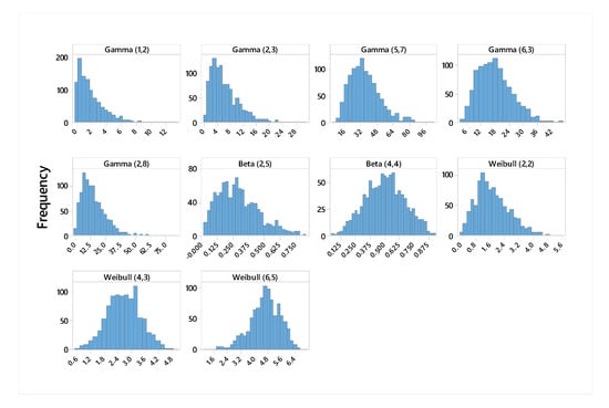
Figure 6. Histogram of non-normal distributions.

Fitting the Generated Data

To ensure that the developed algorithm for generating multivariate non-normal data can perform its intended function, the data must be tested. All generated data are tested using the empirical CDF. Figure 7, Figure 8 and Figure 9 illustrate the CDF for the generated data relative to the theoretical distributions of the corresponding parameters. Three samples are tested using this graph fitting method. In the CDF graphs, almost all the points are the same for the empirical and theoretical data.

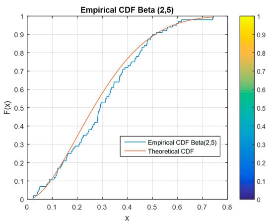
Figure 7. Empirical vs. theoretical cumulative distribution function (CDF) for a beta distribution.

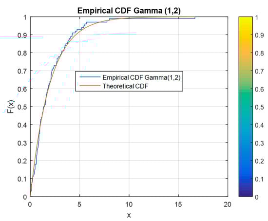
Figure 8. Empirical vs. theoretical CDF for a gamma distribution.

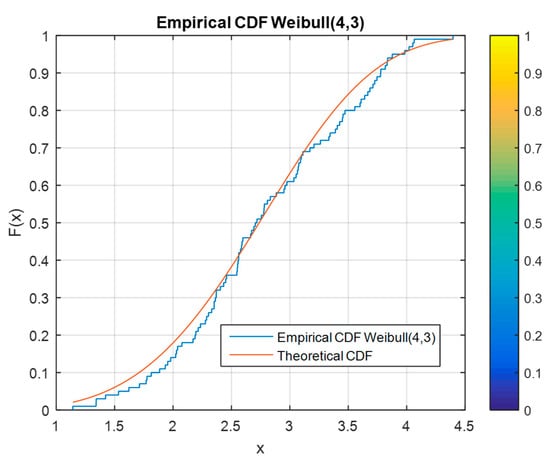
Figure 9. Empirical vs. theoretical CDF for a Weibull distribution.

4.1.2. Case 2

Case Description

In the first case, almost all the samples are right-skewed. However, in real business cases, process data may exhibit right or left (i.e., positive or negative) skewness. To evaluate a robust multivariate capability index, it is necessary to evaluate both types of skewness data, but Abbasi and Niaki’s [41] study does not do so. Thus, a well-known real-world dataset from the literature is utilized. This case is called the connector, and it is obtained from a manufacturer in the computer industry in Taiwan. These process data have a known PNC (0.01). This case study was conducted by Wang [3] and contains a sample of 100 parts that were tested for seven QCs of interest to the manufacturer. These seven QCs are X1 (contact gap X), X2 (contact loop Tp), X3 (LLCR), X4 (contact xTp), X5 (contact loop diameter), X6 (LTGAPY), and X7 (RTGAPY). The specification limits for these seven QCs can be two-sided or one-sided, and they are 0.10 ± 0.04 mm, 0 + 0.50 mm, 11 ± 5 m, 0 + 0.2 mm, 0.55 ± 0.06 mm, 0.07 ± 0.05 mm, and 0.07 ± 0.05 mm, respectively.

Normality Analysis

Figure 10 shows the normality plot for the seven QCs in case 2. The first QC (X1) seems to have a straight probability line fit. Although X1 follows an approximate normal distribution, it still has, however, a relatively small p-value (0.055) for the normality plot. Statistically, all QCs with p-values greater than 0.05 can be treated as normally distributed (X1, X2, X6, and X7). However, these QCs have relatively small p-values except in the case of X2 (p = 0.517). Additionally, the skewness values in Table 5 indicate that all QCs in this case have skewness greater than zero. The QCs in this case (X3, X4, and X5) are not normally distributed.

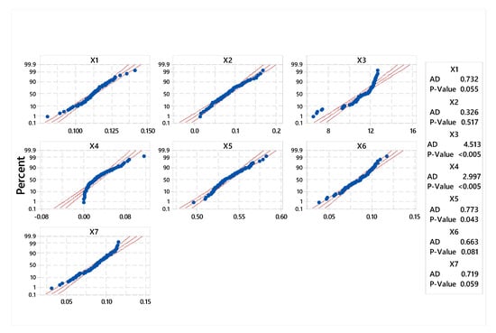
Figure 10. Normal probability plot for X1, X2, X3, X4, X5, X6, and X7.

Table 5. Summary statistics of case 2.

	Variable	Process Statistics				Skewness	Specifications
Statistics		Mean	STD	Minimum	Maximum		LSL	Target	USL
X1		0.113	0.01	0.080	0.141	−0.21	0.06	0.1	0.14
X2		0.083	0.03	0.014	0.167	0.33	-	0	0.5
X3		11.189	1.29	6.511	12.666	−1.79	6	11	16
X4		0.029	0.02	0.000	0.116	1.16	-	0	0.2
X5		0.537	0.02	0.495	0.582	0.45	0.49	0.55	0.61
X6		0.084	0.02	0.038	0.117	−0.53	0.02	0.07	0.12
X7		0.085	0.02	0.031	0.116	−0.61	0.02	0.07	0.12

Table 5 shows the process mean, standard deviation, minimum, and maximum values in addition to the process specifications. It is worth noting that the maximum value of X1 is greater than the upper specification limit, indicating that the process limits are outside of the specification limits, which may lead to an incapable process. All the other data satisfy the specification limits. Furthermore, the skewness column shows that the first and second QCs (X1 and X2) seem to have normal distributions. However, three QCs have left skewness (X3, X6, and X7), and the fourth and fifth QCs (X4 and X5) have the greatest right skewness.

4.2. Root Transformation Method

4.2.1. Validation Process

As mentioned, the root transformation method is established in the literature, and the objective of this section is to validate its results. The purpose of this validation process is to provide confidence that we are applying this method correctly so that we can fairly compare its performance to those of our implemented methods using real and simulated examples. The validation process starts with generating the data used in this method, as discussed in Section 3. After obtaining the desired data, this method is modelled using MATLAB software to simulate the data and obtain multivariate non-normal PCIs for each sample. The simulation study is designed to produce averages over 1000 replications with a sample size of 1,000,000 in each replication.

4.2.2. Comparing the Validation with the Original Outputs

To validate our model, the simulation outputs should not be significantly different from the outputs in the literature. In general, the validation model performs similarly. The outputs are illustrated in Figure 11, which shows that the literature and validation results are very close to each other, especially for gamma distribution. However, there is a slight difference in beta and Weibull distribution, since the validation results are closer to the actual results than those in published results.

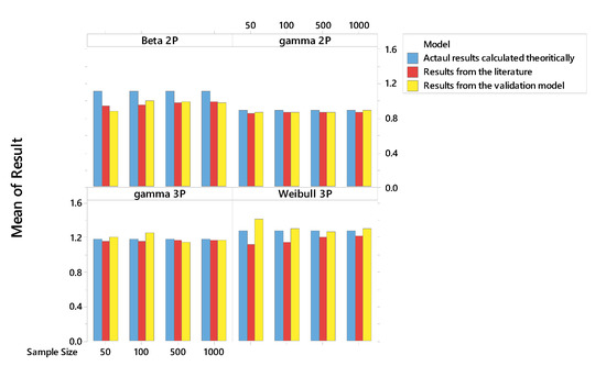
Figure 11. Validation results compared with literature and actual results.

Additionally, a one-way analysis of variance (ANOVA) test is conducted to make inferences about the differences between the validation, literature, and actual results. Table 6 shows the ANOVA for the three results. The model p-value is 0.403, which is greater than the significance level α = 0.05. Consequently, it can be concluded that the three different results do not differ significantly.

Table 6. ANOVA between validation, literature, and actual results.

Source	Degrees of Freedom	Sum of Squares	Mean Squares	F-Value	p-Value
Model	2	0.04676	0.02338	0.93	0.403
Error	45	1.13434	0.02521
Total	47	1.18110

4.2.3. Model Outputs

The simulation study results are presented in Table 7. The root transformation method performs well in calculating multivariate PCIs for right-skewed data. As the data have large positive skewness values, this method performs well in estimating multivariate process capabilities. For example, all the gamma distributed samples have relatively large positive skewness values. Thus, the corresponding estimated multivariate PCIs are very close to the actual values. However, the samples with negative skewness exhibit slightly greater differences between the actual and estimated multivariate PCIs.

Table 7. Multivariate process capability indices (PCIs) using the root transformation method.

Case 1/Distribution	n	URL	$\mathit{\alpha }$	$\mathit{\beta }$	Correlation	Results
						Article	Validation	Actual
gamma	50					0.862	0.864	0.89
	100	13	1	2	1, 0.49	0.873	0.865
	500	26	2	3	0.49, 1	0.873	0.872
	1000					0.873	0.888
gamma	50	130	5	7	1, −0.37, 0.58	1.161	1.208	1.18
	100	58	6	3	−0.37, 1, −0.28	1.151	1.258
	500	150	2	8	0.58, –0.28, 1	1.163	1.148
	1000					1.172	1.172
beta	50					0.939	0.885	1.12
	100	1	2	5	1, 0.79	0.949	1.000
	500	1	4	4	0.79, 1	0.982	0.997
	1000					0.995	0.975
Weibull	50	7	2	2	1, 0.28, 0.58	1.114	1.411	1.28
	100	9	4	3	0.28, 1, 0.49	1.147	1.298
	500	10	6	6	0.58, 0.49, 1	1.199	1.267
	1000					1.213	1.297
Case 2	n	LSL	Target	USL	PNC estimated	PNC actual	Cp estimated	Cp actual
X1	100	0.06	0.1	0.14	0.083	0.01	0.463	0.775
X2		-	0	0.5
X3		6	11	16
X4		-	0	0.2
X5		0.49	0.55	0.61
X6		0.02	0.07	0.12
X7		0.02	0.07	0.12

Although the root transformation method performs well in estimating multivariate PCIs for right-skewed data, it cannot precisely estimate the performances of left-skewed processes. Consequently, this issue limits the use of the root transformation method presented by Abbasi and Niaki [41].

Case 2 contains right- and left-skewed data, and the root method fails to estimate its performance even though this method estimates the performance in case 1 more precisely. Specifically, this method cannot reduce the skewness of left-skewed data. Table 8 presents the skewness of the QCs in case 2 before and after the root transformation. It is clear that X1, X3, X6, and X7 originally have negative skewness and still exhibit the same skewness after the root transformation.

Table 8. Skewness of case 2 quality characteristics (QCs) before and after root transformation.

Variables	X1	X2	X3	X4	X5	X6	X7
Original	−0.21	0.33	−1.79	1.16	0.45	−0.53	−0.61
Transformed	−0.22	0.05	−1.79	0.02	0.38	−0.53	−0.61

4.3. Box–Cox Method

This section presents and discusses the results of the implemented method for estimating multivariate non-normal PCIs using the Box–Cox method. In this subsection, we conduct a simulation study to understand whether our implemented estimation methodology works better than the root transformation method. Although this method performs similarly to the method proposed in the literature (i.e., the root method) for right-skewed data, it outperforms it in estimating left-skewed data. Table 9 presents the multivariate non-normal PCIs using the Box–Cox method.

Table 9. Multivariate non-normal process capability results from the Box–Cox method.

Case 1				Cp
Distribution	# QCs	Sample Size	Root Method	Box–Cox	Johnson	Actual
gamma	2	50	0.864	0.87	0.875	0.89
		100	0.865	0.92	0.863
		500	0.872	0.85	0.882
		1000	0.888	0.85	0.969
	3	50	1.208	0.79	1.141	1.18
		100	1.258	1.05	1.288
		500	1.148	1.11	1.199
		1000	1.172	1.18	1.300
beta	2	50	0.885	0.89	0.926	1.12
		100	1.000	0.98	1.182
		500	0.997	0.97	1.145
		1000	0.975	0.95	1.103
Weibull	3	50	1.411	1.03	1.685	1.28
		100	1.298	1.27	1.468
		500	1.267	1.27	1.276
		1000	1.297	1.22	1.444
Case 2			0.463	0.696	0.737	0.775

4.4. Johnson Multivariate Non-Normal Process Capability Method

A second method for estimating the efficacy of non-normal processes is discussed in this section. This method depends on the Johnson transformation in addition to heuristic search and prediction techniques. The performance of this method is determined by comparing the values of the resulting multivariate non-normal PCIs to the actual values. Table 10 shows the multivariate PCI based on the Johnson method. The results show that the Johnson method performs well in estimating the efficacy of multivariate non-normal processes.

Table 10. Multivariate PCI based on the Johnson method.

Case	Distribution	n	Johnson	Actual
Case 1	gamma	50	0.875	0.89
		100	0.863
		500	0.882
		1000	0.969
	gamma	50	1.141	1.18
		100	1.288
		500	1.199
		1000	1.300
	beta	50	0.926	1.12
		100	1.182
		500	1.145
		1000	1.103
	Weibull	50	1.685	1.28
		100	1.468
		500	1.276
		1000	1.444
Case 2	Real-world data	100	0.737	0.775

4.5. Comparing the Performances of the Root, Box–Cox, and Johnson Methods

The performances of the three studied methods for estimating multivariate non-normal process capabilities is illustrated in Figure 12 and Figure 13 to provide a basis for comparing the two implemented methods with the method from the literature. The figures show that the three methods have almost the same performance in case 1, whereas the implemented methods perform better than the method from the literature in case 2. The multivariate non-normal PCI in case 2 using the Johnson method equals 0.737, which is very close to the actual value (0.78). The Box–Cox method also performs better (0.696) than the method from the literature does (root method (0.463)).

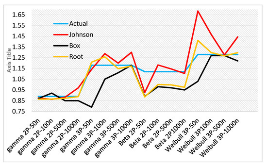
Figure 12. Comparison of the performances of three multivariate process capability methods in case 1.

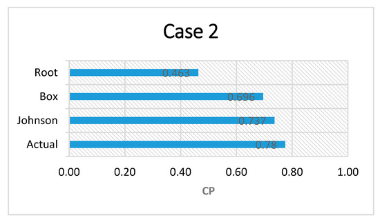
Figure 13. Comparison of the performances of three multivariate process capability methods in case 2.

5. Conclusion and Recommendations

5.1. Conclusions

This study aimed to identify effective models for estimating multivariate non-normal PCIs. The implementations of various transformation techniques in this study show that the type of transformation is an important factor to consider when designing PCIs. The results indicate that the performances of process capability estimations for multivariate non-normal data differ across different transformation techniques.

Whereas the root transformation limits the estimation of multivariate non-normal process capabilities to right-skewed data, this study implements general transformations for both types of skewness. The study replicated the root transformation model and extended it by applying Box–Cox and Johnson transformations. The results presented show that the Box–Cox and Johnson transformations outperform the root transformation in estimating multivariate process capabilities for right- and left-skewed data. In the first case, the three methods perform similarly. However, the Box–Cox and Johnson methods provide more precise results in case 2.

The research in this study confirms an existing method for multivariate non-normal process capability analysis and further improves its performance because it extends the method to all types of skewness. Furthermore, the improved method is easy for quality practitioners to use.

5.2. Recommendations and Future Research

The implementation of different transformation techniques in this study shows that performance varies from one transformation technique to another. Additionally, differences arise when using the same transformation technique. Consequently, research gaps still exist, and filling these gaps may lead to more precise performance evaluation of multivariate QCs with non-normal distributions. These gaps can be sorted into two main groups. The first group is associated with developing and investigating more transformation techniques that can provide better results than the existing techniques can. In this regard, researchers can also validate other methods for estimating Johnson transformation parameters, such as the method of moments. The second group of research opportunities stems from noting that the performances of specific transformation techniques differ from one QC to another. These differences can be investigated alongside analyses of QC properties. Such studies may conclude that each transformation technique performs well for specific QC data with specific properties. Moreover, research in this field can be conducted using other criteria besides the skewness of QC data. Finally, depending on the outcomes of research into these gaps, a software package can be developed for industry practitioners. This package can optimize performance evaluation for multivariate QC data, which can facilitate the implementation of multivariate PCIs for non-specialists.

References

- Albing, M. Process Capability Analysis with Focus on Indices for One-Sided Specification Limits. Ph.D. Thesis, Luleå Tekniska Universitet, Luleå, Sweden, 2006. [Google Scholar]
- Hahn, G.J.; Hill, W.J.; Hoerl, R.; Zinkgraf, S.A. The impact of Six Sigma improvement—A glimpse into the future of statistics. Am. Stat. 1999, 53, 208–215. [Google Scholar]
- Wang, F. Quality evaluation of a manufactured product with multiple characteristics. Qual. Reliab. Eng. Int. 2006, 22, 225–236. [Google Scholar] [CrossRef]
- Taam, W.; Subbaiah, P.; Liddy, J.W. A note on multivariate capability indices. J. Appl. Stat. 1993, 20, 339–351. [Google Scholar] [CrossRef]
- Chen, H. A multivariate process capability index over a rectangular solid tolerance zone. Stat. Sin. 1994, 4, 749–758. [Google Scholar]
- Shahriari, H.; Hubele, N.; Lawrence, F. A Multivariate Process Capability Vector. Proc. 4th Ind. Eng. Res. Conf. 1995, 1, 304–309. [Google Scholar]
- Braun, L. New Methods in Multivariate Statistical Process Control(MSPC). 2001, 1–12. Available online: http://citeseerx.ist.psu.edu/viewdoc/download?doi=10.1.1.569.9886&rep=rep1&type=pdf (accessed on 7 November 2019).
- Castagliola, P.; Castellanos, J.-V.G.; Management, Q. Capability indices dedicated to the two quality characteristics case. Qual. Technol. Quant. Manag. 2005, 2, 201–220. [Google Scholar] [CrossRef]
- Bothe, D.R. A capability index for multiple process streams. Qual. Eng. 1999, 11, 613–618. [Google Scholar] [CrossRef]
- Wang, F.K.; Du, T.C.T. Using principal component analysis in process performance for multivariate data. Omega-Int. J. Manag. Sci. 2000, 28, 185–194. [Google Scholar] [CrossRef]
- Boyles, R.A. Brocess Capability with Asymmetric Tolerances. Commun. Stat.-Simul. Comput. 1994, 23, 615–643. [Google Scholar] [CrossRef]
- Davis, R.D.; Kaminsky, F.C.; Saboo, S. Process capability analysis for processes with either a circular or a spherical tolerance zone. Qual. Eng. 1992, 5, 41–54. [Google Scholar] [CrossRef]
- Yeh, A.B.; Bhattacharya, S. A robust process capability index. Communications in Statistics-Simulation and Computation. Commun. Stat.-Simul. Comput. 1998, 27, 565–589. [Google Scholar] [CrossRef]
- Veevers, A. Viability and capability indexes for multiresponse processes. J. Appl. Stat. 1998, 25, 545–558. [Google Scholar] [CrossRef]
- Dianda, D.F.; Quaglino, M.B.; Pagura, J.A. Impact of measurement errors on the performance and distributional properties of the multivariate capability index. AStA Adv. Stat. Anal. 2018, 102, 117–143. [Google Scholar] [CrossRef]
- Peruchi, R.S.; Junior, P.R.; Brito, T.G.; Largo, J.J.J.; Balestrassi, P.P. Multivariate process capability analysis applied to 52100 hardened steel turning. Int. J. Adv. Manuf. Technol. 2018, 95, 3513–3522. [Google Scholar] [CrossRef]
- Chatterjee, M.; Chakraborty, A.K. Unification of some multivariate process capability indices for asymmetric specification region. Stat. Neerl. 2017, 71, 286–306. [Google Scholar] [CrossRef]
- Dianda, D.F.; Quaglino, M.B.; Pagura, J.A. Distributional Properties of Multivariate Process Capability Indices under Normal and Non-Normal Distributions. Qual. Reliab. Eng. Int. 2017, 33, 275–295. [Google Scholar] [CrossRef]
- Vasquez, M.; Ramirez, G.; Garcia, T. A Multivariate Process Capability Index Based on Non-Conforming Probability, an Illustration about Monitoring the Quality of a Clarified Water Loop. Ingenieria Uc 2016, 23, 319–326. [Google Scholar]
- Pan, J.N.; Li, C.I.; Shih, W.C. New multivariate process capability indices for measuring the performance of multivariate processes subject to non-normal distributions. Int. J. Qual. Reliab. Manag. 2016, 33, 42–61. [Google Scholar] [CrossRef]
- Ciupke, K. Multivariate Process Capability Index Based on Data Depth Concept. Qual. Reliab. Eng. Int. 2016, 32, 2443–2453. [Google Scholar] [CrossRef]
- Ciupke, K. Multivariate Process Capability Vector Based on One-Sided Model. Qual. Reliab. Eng. Int. 2015, 31, 313–327. [Google Scholar] [CrossRef]
- Mondal, S.C. A study of multivariate process capability indices in manufacturing processes. In Proceedings of the 2015 IEEE International Conference on Industrial Engineering and Engineering Management (IEEM), Singapore, 6–9 December 2015; pp. 1382–1386. [Google Scholar]
- Pan, J.-N.; Huang, W.K.C. Developing New Multivariate Process Capability Indices for Autocorrelated Data. Qual. Reliab. Eng. Int. 2015, 31, 431–444. [Google Scholar] [CrossRef]
- Siman, M. Multivariate Process Capability Indices: A Directional Approach. Commun. Stat.-Theory Methods 2014, 43, 1949–1955. [Google Scholar] [CrossRef]
- Zhang, M.; Wang, G.A.; He, S.G.; He, Z. Modified Multivariate Process Capability Index Using Principal Component Analysis. Chin. J. Mech. Eng. 2014, 27, 249–259. [Google Scholar] [CrossRef]
- Tano, I.; Vannman, K. A Multivariate Process Capability Index Based on the First Principal Component Only. Qual. Reliab. Eng. Int. 2013, 29, 987–1003. [Google Scholar] [CrossRef]
- Das, N.; Dwivedi, P.S. Multivariate Process Capability Index: A Review and Some Results. Econ. Qual. Control 2013, 28, 151–166. [Google Scholar] [CrossRef]
- Bashiri, M.J.M.; Amiri, A. A New Multivariate Process Capability Index Under Both Unilateral and Bilateral Quality Characteristics. Qual. Reliab. Eng. Int. 2012, 28, 925–941. [Google Scholar]
- Niavarani, M.R.; Noorossana, R.; Abbasi, B. Three New Multivariate Process Capability Indices. Commun. Stat.-Theory Methods 2012, 41, 341–356. [Google Scholar] [CrossRef]
- Scagliarini, M. Multivariate process capability using principal component analysis in the presence of measurement errors. AStA Adv. Stat. Anal. 2011, 95, 113–128. [Google Scholar] [CrossRef]
- Pan, J.N.; Lee, C.Y. New capability indices for evaluating the performance of multivariate manufacturing processes. Qual. Reliab. Eng. Int. 2010, 26, 3–15. [Google Scholar] [CrossRef]
- Ahmad, S.; Abdollahian, M.; Zeephongsekul, P.; Abbasi, B. Multivariate nonnormal process capability analysis. Int. J. Adv. Manuf. Technol. 2009, 44, 757–765. [Google Scholar] [CrossRef]
- Wen, D.C.; Lv, H. Multivariate Process Capability Index Based on the Additivity of Normal Distribution. In Proceedings of the 2008 4th International Conference on Wireless Communications, Networking and Mobile Computing, Dalian, China, 12–14 October 2008; IEEE: New York, NY, USA, 2008. [Google Scholar]
- Pearn, W.L.; Wang, F.K.; Yen, C.H. Multivariate capability indices: Distributional and inferential properties. J. Appl. Stat. 2007, 34, 941–962. [Google Scholar] [CrossRef]
- Wang, C.H. Constructing multivariate process capability indices for short-run production. Int. J. Adv. Manuf. Technol. 2005, 26, 1306–1311. [Google Scholar] [CrossRef]
- Wang, F.; Chen, J.C. Capability index using principal components analysis. Qual. Eng. 1998, 11, 21–27. [Google Scholar] [CrossRef]
- Castagliola, P. Evaluation of non-normal process capability indices using Burr’s distributions. Qual. Eng. 1996, 8, 587–593. [Google Scholar] [CrossRef]
- Pearn, W.L.; Shiau, J.J.H.; Tai, Y.T.; Li, M.Y. Capability Assessment for Processes with Multiple Characteristics: A Generalization of the Popular Index C-pk. Qual. Reliab. Eng. Int. 2011, 27, 1119–1129. [Google Scholar] [CrossRef]
- Shiau, J.J.H.; Yen, C.L.; Pearn, W.; Lee, W.T. Yield-related process capability indices for processes of multiple quality characteristics. Qual. Reliab. Eng. Int. 2013, 29, 487–507. [Google Scholar] [CrossRef]
- Abbasi, B.; Niaki, S.T.A. Estimating process capability indices of multivariate nonnormal processes. Int. J. Adv. Manuf. Technol. 2010, 50, 823–830. [Google Scholar] [CrossRef]
- Kotz, S.; Lovelace, C.R. Process Capability Indices in Theory and Practice; Arnold: London, UK, 1998. [Google Scholar]
- Clements, J.A. Process Capability Calculations for Non-Normal Distributions. Qual. Prog. 1989, 22, 95–97. [Google Scholar]
- Somerville, S.E.; Montgomery, D.C.J.Q.E. Process capability indices and non-normal distributions. Qual. Eng. 1996, 9, 305–316. [Google Scholar] [CrossRef]
- Deleryd, M.; Management, R. On the gap between theory and practice of process capability studies. Int. J. Qual. Reliab. Manag. 1998, 15, 178–191. [Google Scholar] [CrossRef]
- Wu, H.; Wang, J.; Liu, T. Discussions of the Clements-based process capability indices. In Proceedings of the 1998 CIIE National Conference, Hsin-Hua, Taiwan, December 1998; pp. 561–566. [Google Scholar]
- Kotz, S.; Johnson, N.L. Process capability indices—A review, 1992–2000. J. Qual. Technol. 2002, 34, 2–19. [Google Scholar] [CrossRef]
- Liu, P.-H.; Chen, F.-L. Process capability analysis of non-normal process data using the Burr XII distribution. Int. J. Adv. Manuf. Technol. 2006, 27, 975–984. [Google Scholar] [CrossRef]
- Piao, C.; Zhi-Sheng, Y. A systematic look at the gamma process capability indices. Eur. J. Oper. Res. 2018, 265, 589–597. [Google Scholar]
- Li, C.-J.; Deng, W.-P.; Cao, Y.-Y.; Bao, Y. Process capability analysis in non-normality based on Box-Cox transformation and Johnson transformation. J. Qiqihar Univ. (Nat. Sci. Ed.) 2015, 1, 66–70. [Google Scholar]
- Bernardo, J.M.; Irony, T.Z. A general multivariate Bayesian process capability index. J. R. Stat. Soc. Ser. D 1996, 45, 487–502. [Google Scholar] [CrossRef]
- Wang, F.-K.; Hubele, N.F. Quality evaluation using geometric distance approach. Int. J. Reliab. Qual. Saf. Eng. 1999, 6, 139–153. [Google Scholar] [CrossRef]
- Pal, S.J.Q.E. Evaluation of nonnormal process capability indices using generalized lambda distribution. Qual. Eng. 2004, 17, 77–85. [Google Scholar] [CrossRef]
- Chen, K.-S.; Hsu, C.-H.; Wu, C.-C. Process capability analysis for a multi-process product. Int. J. Adv. Manuf. Technol. 2006, 27, 1235–1241. [Google Scholar] [CrossRef]
- Niaki, S.T.A.; Abbasi, B. Skewness reduction approach in multi-attribute process monitoring. Commun. Stat. Theory Methods 2007, 36, 2313–2325. [Google Scholar] [CrossRef]
- Perakis, M.; Xekalaki, E. On the Implementation of the Principal Component Analysis-Based Approach in Measuring Process Capability. Qual. Reliab. Eng. Int. 2012, 28, 467–480. [Google Scholar] [CrossRef]
- Dharmasena, L.; Zeephongsekul, P. A new process capability index for multiple quality characteristics based on principal components. Int. J. Prod. Res. 2016, 54, 4617–4633. [Google Scholar] [CrossRef]
- Shaoxi, W.; Mingxin, W.; Xiaoya, F.; Shengbing, Z.; Ru, H. A multivariate process capability index with a spatial coefficient. J. Semicond. 2013, 34. [Google Scholar] [CrossRef]
- Gu, K.; Jia, X.; Liu, H.; You, H. Yield-based capability index for evaluating the performance of multivariate manufacturing process. Qual. Reliab. Eng. Int. 2015, 31, 419–430. [Google Scholar] [CrossRef]
- Tiwari, V.; Singh, N. Process capability index for bivariate exponentially distributed quality characteristics and its sampling properties. Commun. Stat.-Theory Methods 2017, 46, 11099–11109. [Google Scholar] [CrossRef]
- Box, G.E.; Cox, D.R. An analysis of transformations. J. R. Stat. Soc. Ser. B 1964, 26, 211–243. [Google Scholar] [CrossRef]
- Johnson, N.L.J.B. Systems of frequency curves generated by methods of translation. Biometrika 1949, 36, 149–176. [Google Scholar] [CrossRef]
- Montgomery, D.C. Introduction to Statistical Quality Control, 2005; John Wiley& Sons: New York, NY, USA, 2017. [Google Scholar]
- Juran, J.; Gryna, M.F., Jr.; Bingham, R.S., Jr. Quality costs. Qual.Control Handb. 1974, 3, 5.1. [Google Scholar]
- Pearn, W.; Kotz, S. Application of Clements’ Method for Calculating Second-and Third-Generation Process Capability Indices for Non-Normal Personian Populations. Qual. Eng. 1994, 7. [Google Scholar] [CrossRef]
- Kane, V. Process Capability Indexes. J. Qual. Technol. 1986, 18, 41–52. [Google Scholar] [CrossRef]
- Telmoudi, P.R. A Multi-Stream Process Capability Assessment Using a Nonconformity Ratio Based Desirability Function, 2005. Available online: http://citeseerx.ist.psu.edu/viewdoc/summary?doi=10.1.1.428.3059 (accessed on 7 November 2019).
© 2019 by the authors. Licensee MDPI, Basel, Switzerland. This article is an open access article distributed under the terms and conditions of the Creative Commons Attribution (CC BY) license (http://creativecommons.org/licenses/by/4.0/).