A Modifier-Adaptation Strategy towards Offset-Free Economic MPC

Abstract

We address in the paper the problem of designing an economic model predictive control (EMPC) algorithm that asymptotically achieves the optimal performance despite the presence of plant-model mismatch. To motivate the problem, we present an example of a continuous stirred tank reactor in which available EMPC and tracking model predictive control (MPC) algorithms do not reach the optimal steady state operation. We propose to use an offset-free disturbance model and to modify the target optimization problem with a correction term that is iteratively computed to enforce the necessary conditions of optimality in the presence of plant-model mismatch. Then, we show how the proposed formulation behaves on the motivating example, highlighting the role of the stage cost function used in the finite horizon MPC problem.

1. Introduction

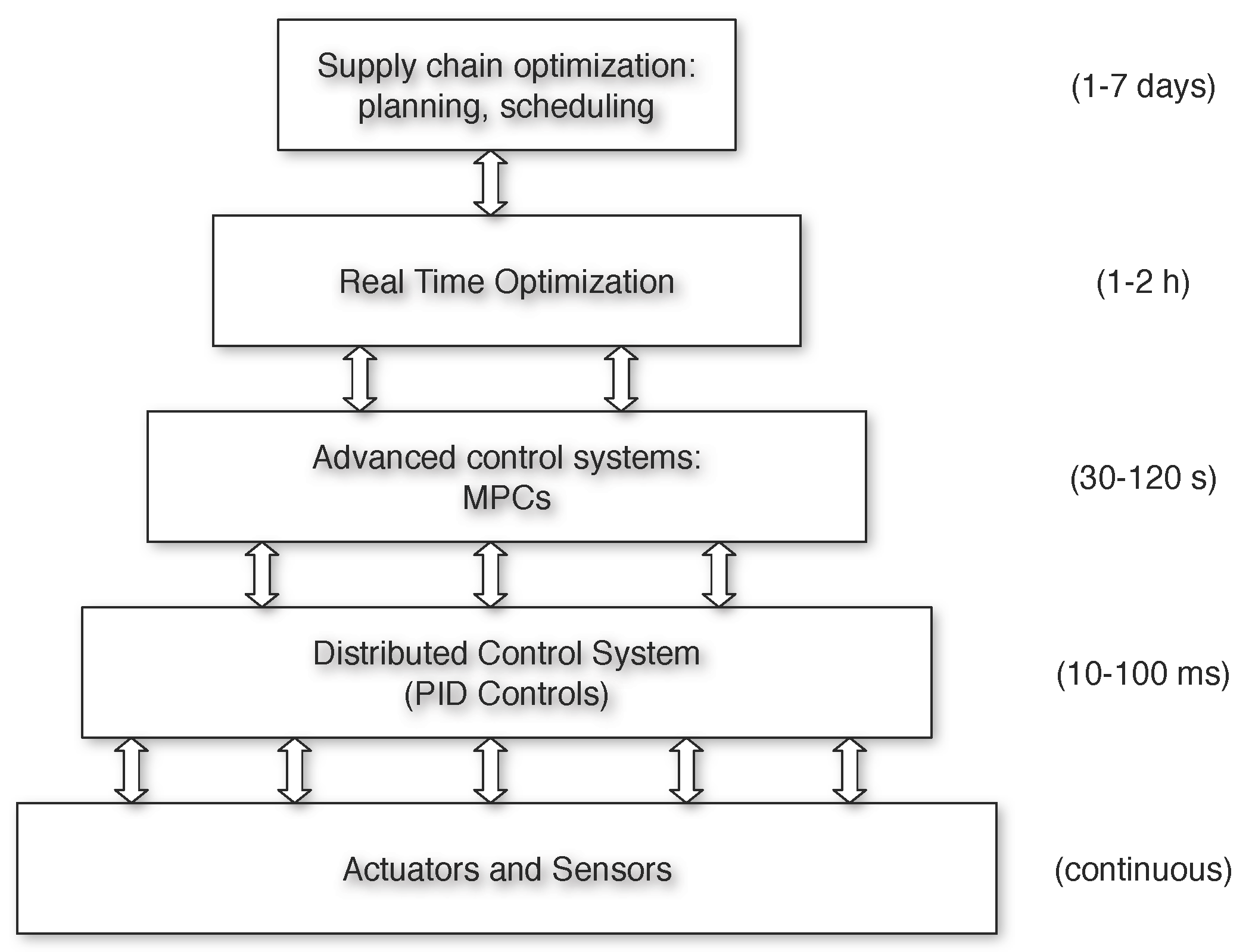
Optimization-based controllers, in general, and model predictive control (MPC) systems, in particular, represent an extraordinary success case in the history of automation in the process industries [1]. MPC algorithms exploit a (linear or nonlinear) dynamic model of the process and numerical optimization algorithms to guide a process to a setpoint reliably, while fulfilling constraints on outputs and inputs. The optimal steady-state setpoint is usually provided by an upper layer, named real-time optimization (RTO), that is dedicated to economic steady-state optimization. The typical hierarchical architecture for economic optimization and control in the process industries is depicted in Figure 1. For an increasing number of applications, however, this separation of information and purpose is no longer optimal nor desirable [2]. An alternative to this decomposition is to take the economic objective directly as the objective function of the control system. In this approach, known as economic model predictive control (EMPC), the controller optimizes directly, in real time, the economic performance of the process, rather than tracking a setpoint.

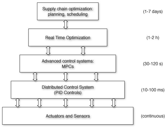
Figure 1. Typical hierarchical optimization and control structure in process systems.

MPC being a model-based optimization algorithm, in the presence of plant-model mismatch or unmeasured disturbances, it can come across offset problems. Non-economically optimum stationary points can also be the result of a plant-model mismatch in model-based RTO. However, as explained later, some RTO algorithms do not use a model, i.e., extremum-seeking control [3,4], so in this case, the mismatch issue can be associated with unmeasured disturbances. The offset correction in tracking MPC algorithms has been deeply exploited and analyzed. Muske and Badgwell [5] and Pannocchia and Rawlings [6] first introduced the concept of general conditions that allow zero steady-state offset with respect to external setpoints. The general approach is to augment the nominal system with disturbances, i.e., to build a disturbance model and to estimate the state and disturbance from output measurements. A recent review about disturbance models and offset-free MPC design can also be found in [7]. Furthermore, in the RTO literature, many works are focused on plant-model mismatch issues. RTO typically proceeds using an iterative two-step approach [8,9], namely an identification step followed by an optimization step. The idea is to repeatedly estimate selected uncertain model parameters and to use the updated model to generate new inputs via optimization. Other alternative options do not use a process model online to implement the optimization [10,11,12]. Others utilize a nominal fixed process model and appropriate measurements to guide the iterative scheme towards the optimum. In this last field, the term “modifier-adaptation” indicates those fixed-model methods that adapt correction terms (i.e., the modifiers) based on the observed difference between actual and predicted functions or gradients [13,14,15]. Marchetti et al. [16] formalize the concept of using plant measurements to adapt the optimization problem in response to plant-model mismatch, through modifier-adaptation.

As underlined above, the RTO and MPC hierarchical division issue has led to the increased interest in merging the two layers. Many works in the literature consider a combination between RTO and MPC through a target calculation level in the middle that coordinates the communication and guarantees stability to the whole structure calculating the feasible target for the optimal control problem [17,18]. There are also examples of integration between the modifier-adaptation technique and MPC [19]: in this way, the input targets calculated by the MPC are included as equality constraints into the modified RTO problem. In other cases, the target module of the MPC has been modified in various ways, including a new quadratic programming problem that is an approximation of the RTO problem [20].

Another area of the literature aimed at merging the two layers is the so-called dynamic real-time optimization (D-RTO). The objective function of the D-RTO includes an economic objective, subject to a dynamic model of the plant. The optimal control profiles are then determined from the solution of the above dynamic optimization problem and then passed to the underlined MPC layer as trajectory setpoints to follow. The advantages of this formulation in the presence of disturbances have been deeply emphasized in the literature [21,22], also in the case of model-free alternatives [23]. The D-RTO is also seen as a solution for merging economic and control layer, while advances in nonlinear model predictive control and its generalization to deal with economic objective functions taking place [24]. In this sense, a receding horizon closed-loop implementation of D-RTO can be also referred to as economic model predictive control [25].

In the presence of plant-model mismatch, also EMPC can suffer from converging to a non-economically steady-state point and also reaching a steady state different from the one indicated by the target at the same time. The main goal of this work is to build an economic MPC algorithm that, combining the previous ideas of offset-free MPC and modifier-adaptation, achieves the ultimate optimal economic performance despite modeling errors and/or disturbances. In the proposed method, there is no RTO layer because the economic cost function is used directly in the MPC formulation, which however includes a modifier-adaptation scheme.

The rest of this paper is organized as follows. A review of the related technique used in this work is presented in Section 2 along with a motivating example. The proposed method, with a detailed mathematical analysis and description, is presented in Section 3. The algorithm and several variants are then tested over the illustrative example, and the numerical results and associated discussions are reported in Section 4. Finally, Section 5 concludes the paper and presents possible future directions of this methodology.

2. Related Techniques and a Motivating Example

In order to propose an offset-free EMPC algorithm, a review of related concepts and techniques is given. Then, we present a motivating example that shows how neither the standard EMPC formulation nor an offset-free tracking MPC formulation are able to achieve the ultimate optimal economic performance.

2.1. Plant, Model and Constraints

In this paper, we are concerned with the control of time-invariant dynamical systems in the form:

$$\begin{array}{cc}\hfill x_p^{+}& =F_p(x_p,u)\hfill \\ \hfill y& =H_p\left(x_p\right)\hfill \end{array}$$

(1)

in which $x_p\in {\mathbb{R}}^n$, $u\in {\mathbb{R}}^m$, $y\in {\mathbb{R}}^p$ are the plant state, control input and output at a given time, respectively, and $x_p^{+}$ is the successor state. The plant output is measured at each time $k\in \mathbb{I}$. Functions $F_p$: ${\mathbb{R}}^n\times {\mathbb{R}}^m\to {\mathbb{R}}^n$ and $H_p$: ${\mathbb{R}}^n\to {\mathbb{R}}^p$ are not known precisely, but are assumed to be differentiable. In order to design an MPC algorithm, a process model is known:

$$\begin{array}{cc}\hfill x^{+}& =f(x,u)\hfill \\ \hfill y& =h\left(x\right)\hfill \end{array}$$

(2)

in which $x,x^{+}\in {\mathbb{R}}^n$ denote the current and successor model states. The functions f: ${\mathbb{R}}^n\times {\mathbb{R}}^m\to {\mathbb{R}}^n$ and h: ${\mathbb{R}}^n\to {\mathbb{R}}^p$ are assumed to be differentiable. Input and output are required to satisfy the following input and output constraints at all times:

$$u_{min}\le u\le u_{max},y_{min}\le y\le y_{max}$$

(3)

in which $u_{min},u_{max}\in {\mathbb{R}}^m$ and $y_{min},y_{max}\in {\mathbb{R}}^p$ are the bound vectors.

2.2. Offset-Free Tracking MPC

Offset-free MPC algorithms are generally based on an augmented model [5,6,26,27]. The general form of this augmented model can be written as:

$$\begin{array}{cc}\hfill x^{+}& =F(x,u,d)\hfill \\ \hfill d^{+}& =d\hfill \\ \hfill y& =H(x,d)\hfill \end{array}$$

(4)

in which $d\in {\mathbb{R}}^{n_d}$ is the so-called disturbance. The functions F: ${\mathbb{R}}^n\times {\mathbb{R}}^m\times {\mathbb{R}}^{n_d}\to {\mathbb{R}}^n$ and H: ${\mathbb{R}}^n\times {\mathbb{R}}^{n_d}\to {\mathbb{R}}^p$ are assumed to be continuous and consistent with (2), i.e., $F(x,u,0)=f(x,u)$ and $H(x,0)=h\left(x\right)$.

Assumption 1.

The augmented system (4) is observable.

At each time $k\in \mathbb{I}$, given the output measurement $y\left(k\right)$, an observer for (4) is defined to estimate the augmented state ($x\left(k\right),d\left(k\right)$). For simplicity of exposition, only the current measurement of $y\left(k\right)$ is used to update the prediction of ($x\left(k\right),d\left(k\right)$) made at the previous decision time, i.e., a “Kalman filter”-like estimator is used. We define symbols ${\widehat{x}}_{k|k-1}$, ${\widehat{d}}_{k|k-1}$ and ${\widehat{y}}_{k|k-1}$ as the predicted estimate of $x\left(k\right)$, $d\left(k\right)$ and $y\left(k\right)$, respectively, obtained at the previous time $k-1$ using the augmented model (4), i.e.,

$$\begin{array}{cc}\hfill {\widehat{x}}_{k|k-1}& =F({\widehat{x}}_{k-1|k-1},u_{k-1},{\widehat{d}}_{k-1|k-1})\hfill \\ \hfill {\widehat{d}}_{k|k-1}& ={\widehat{d}}_{k-1|k-1}\hfill \\ \hfill {\widehat{y}}_{k|k-1}& =H({\widehat{x}}_{k|k-1},{\widehat{d}}_{k|k-1})\hfill \end{array}$$

(5)

Defining the output prediction error as:

$$e_k=y\left(k\right)-{\widehat{y}}_{k|k-1}$$

(6)

the filtering relations can be written as follows:

$$\begin{array}{cc}\hfill {\widehat{x}}_{k|k}& ={\widehat{x}}_{k|k-1}+{\mathsf{\kappa }}_x\left(e_k\right)\hfill \\ \hfill {\widehat{d}}_{k|k}& ={\widehat{d}}_{k|k-1}+{\mathsf{\kappa }}_d\left(e_k\right)\hfill \end{array}$$

(7)

where ${\widehat{x}}_{k|k}$ and ${\widehat{d}}_{k|k}$ are the filtered estimate of $x\left(k\right)$ and $d\left(k\right)$ in (4) obtained using measurement $y\left(k\right)$. We assume that Relations (5)–(7) form an asymptotically-stable observer for the augmented system (4).

Given the current estimate of the augmented state (${\widehat{x}}_{k|k},{\widehat{d}}_{k|k}$), an offset-free tracking MPC algorithm computes the steady-state target that ensures exact setpoint tracking in the controlled variable. Hence, in general, the following target problem is solved:

$$\begin{array}{c}\underset{x,u,y}{min}{\ell }_s(y-y_{sp},u-u_{sp})\end{array}$$

(8a)

subject to

$$\begin{array}{c}\hfill x=F(x,{\widehat{d}}_{k|k},u)\end{array}$$

(8b)

$$\begin{array}{c}\hfill y=H(x,{\widehat{d}}_{k|k})\end{array}$$

(8c)

$$\begin{array}{c}\hfill u_{min}\le u\le u_{max}\end{array}$$

(8d)

$$\begin{array}{c}\hfill y_{min}\le y\le y_{max}\end{array}$$

(8e)

in which ${\ell }_s$: ${\mathbb{R}}^p\times {\mathbb{R}}^m\to \mathbb{R}$ is the steady-state cost function and $y_{sp}\in {\mathbb{R}}^p$, $u_{sp}\in {\mathbb{R}}^m$ are the output and input setpoints, respectively. We assume (8) is feasible, and we denote its (unique) solution as $(x_{s,k},u_{s,k},y_{s,k})$. Typically, ${\ell }_s(·)$ is positive definite in the first argument (output steady-state error) and semidefinite in the second argument (input steady-state error), and relative input and output weights are chosen to ensure that $y_{s,k}\to y_{sp}$ whenever constraints allow it.

Let $\mathit{x}=\{x_0,x_1,\dots ,x_N\}$ and $\mathit{u}=\{u_0,u_1,\dots ,u_{N-1}\}$ be, respectively, a state sequence and an input sequence. The finite horizon optimal control problem (FHOCP) solved at each time is the following:

$$\begin{array}{c}\underset{\mathit{x},\mathit{u}}{min}\sum _{i=0}^{N-1}{\ell }_{QP}\left(x_i-x_{s,k},u_i-u_{s,k}\right)+V_f\left(x_N-x_{s,k}\right)\end{array}$$

(9a)

subject to

$$\begin{array}{c}\hfill x_0={\widehat{x}}_{k|k},\end{array}$$

(9b)

$$\begin{array}{c}\hfill x_{i+1}=F(x_i,{\widehat{d}}_{k|k},u_i),i=0,\dots ,N-1\end{array}$$

(9c)

$$\begin{array}{c}\hfill u_{min}\le u_i\le u_{max},i=0,\dots ,N-1\end{array}$$

(9d)

$$\begin{array}{c}\hfill y_{min}\le H(x_i,{\widehat{d}}_{k|k})\le y_{max}i=0,\dots ,N-1\end{array}$$

(9e)

$$\begin{array}{c}\hfill x_N=x_{s,k}\end{array}$$

(9f)

in which ${\ell }_{QP}$: ${\mathbb{R}}^n\times {\mathbb{R}}^m\to {\mathbb{R}}_{\ge 0}$ is a strictly positive definite convex function. $V_f$: ${\mathbb{R}}^n\to {\mathbb{R}}_{\ge 0}$ is a terminal cost function, which may vary depending on the specific MPC formulation, according to the usual stabilizing conditions [28]. Assuming Problem (9) to be feasible, its solution is denoted by $({\mathit{x}}_k^0,{\mathit{u}}_k^0)$, and the associated receding horizon implementation is given by:

$$u_k=u_{0,k}^0$$

(10)

As the conclusion of this discussion, the following result holds true [5,6,29].

Proposition 1.

Consider a system controlled by the MPC algorithm as described above. If the closed-loop system is stable, then the output prediction error goes to zero, i.e.,

$$\underset{k\to \infty }{lim}y\left(k\right)-{\widehat{y}}_{k|k-1}=0$$

(11)

Furthermore, if input constraints are not active at steady state, there is zero offset in the controlled variables, that is:

$$\underset{k\to \infty }{lim}y\left(k\right)-y_{sp}=0$$

(12)

2.3. Economic MPC

As can be seen from Figure 1, setpoints $(y_{sp},u_{sp})$ that enter in (8) come from the upper economic layer referred to as the RTO. This hierarchical division may limit the achievable flexibility and economic performance that many processes nowadays request. There are several proposals to improve the effective use of dynamic and economic information throughout the hierarchy. As explained in Section 1, the first approach to this merging is the D-RTO. While many D-RTO structures have been proposed throughout the literature [23,30,31], many of the two-layered D-RTO and MPC systems proposed are characterized by a lack of rigorous theoretical treatment, including the constraints. However, as can be seen in the above cited literature, the D-RTO formulations still consider the presence of both RTO and MPC in separated layers. Instead of moving the dynamic characteristic to the RTO level, the interest here is to move economic information into the control layer. This approach involves modifying the traditional tracking objective function in (9) and the target cost function in (8) directly with the economic stage cost function used in the RTO layer. In this latter case, the formulation takes the name of economic MPC (EMPC) [32]. It has to be underlined that, in this case, the economic optimization is provided only by the EMPC layer, while the RTO one is completely eliminated.

In standard MPC, the objective is designed to ensure asymptotic stability of the desired steady state. This is accomplished by choosing the stage cost to be zero at the steady-state target pair, denoted $(x_s,u_s)$, and positive elsewhere, i.e.,

$$0={\ell }_{QP}(x_s,u_s)\le {\ell }_{QP}(x,u)\mathrm{for}\mathrm{all}\mathrm{admissible}(x,u)$$

(13)

In EMPC, instead, the operating cost of the plant is used directly as the stage cost in the FHOCP objective function. As a consequence, it may happen that ${\ell }_e(x_s,u_s)>{\ell }_e(x,u)$ for some feasible pair $(x,u)$ that is not a steady state. This possibility has significant impact on stability and convergence properties. In fact, while a common approach in the tracking MPC is to use the optimal cost as a Lyapunov function for the closed-loop system to prove its stability, in the EMPC formulation, due to the fact that (13) does not hold, these stability arguments fail. Hence, for certain systems and cost functions, oscillating solutions may be economically more profitable than steady-state ones, giving rise to the concept of average asymptotic performance of economic MPC, which is deeply developed in [32,33]. Despite that, in the literature, there are also formulations of the Lyapunov-based EMPC by taking advantage of an auxiliary MPC problem solution [34,35].

In this work, we assume that operating at steady-state is more profitable than an oscillating behavior. Hence, in order to delineate the concept of convergence in EMPC, two other properties may be useful: dissipativity [32,36] and turnpike [37,38]. These properties play a key role in the analysis and design of schemes for D-RTO and EMPC. It is shown also that in a continuous-time form, the dissipativity of a system with respect to a steady state implies the existence of a turnpike at this steady state and optimal stationary operation at this steady state [39,40]. An extensive review about EMPC control methods can be found in [41,42].

The starting EMPC algorithm considered in this work is taken from [29] and includes an offset-free disturbance model as described in Section 2.2. Given the current state and disturbance estimate (${\widehat{x}}_{k|k},{\widehat{d}}_{k|k}$), the economic steady-state target is given by:

$$\begin{array}{c}\underset{x,u,y}{min}{\ell }_e(y,u)\end{array}$$

(14a)

subject to

$$\begin{array}{c}\hfill x=F(x,{\widehat{d}}_{k|k},u)\end{array}$$

(14b)

$$\begin{array}{c}\hfill y=H(x,{\widehat{d}}_{k|k})\end{array}$$

(14c)

$$\begin{array}{c}\hfill u_{min}\le u\le u_{max}\end{array}$$

(14d)

$$\begin{array}{c}\hfill y_{min}\le y\le y_{max}\end{array}$$

(14e)

in which ${\ell }_e$: ${\mathbb{R}}^p\times {\mathbb{R}}^m\to \mathbb{R}$ is the economic cost function defined in terms of output and input. Notice that the arguments of the economic cost function are measurable quantities. Let $(x_{s,k},u_{s,k},y_{s,k})$ be the steady-state target triple solution to (14). Then, the FHOCP solved at each time is given by:

$$\begin{array}{c}\underset{\mathit{x},\mathit{u}}{min}\sum _{i=0}^{N-1}{\ell }_e(H(x_i,{\widehat{d}}_{k|k}),u_i)\end{array}$$

(15a)

subject to

$$\begin{array}{c}\hfill x_0={\widehat{x}}_{k|k},\end{array}$$

(15b)

$$\begin{array}{c}\hfill x_{i+1}=F(x_i,{\widehat{d}}_{k|k},u_i),i=0,\dots ,N-1\end{array}$$

(15c)

$$\begin{array}{c}\hfill u_{min}\le u_i\le u_{max},i=0,\dots ,N-1\end{array}$$

(15d)

$$\begin{array}{c}\hfill y_{min}\le H(x_i,{\widehat{d}}_{k|k})\le y_{max},i=0,\dots ,N-1\end{array}$$

(15e)

$$\begin{array}{c}\hfill x_N=x_{s,k}\end{array}$$

(15f)

While several formulations of economic MPC are possible, in this work, we use a terminal equality constraint to achieve asymptotic stability [36]. We remark that the target equilibrium $x_{s,k}$ is recomputed at each decision time by the target calculation problem (14).

2.4. A Motivating Example

2.4.1. Process and Optimal Economic Performance

In order to motivate this work, we show the application of EMPC formulations to a chemical reactor to highlight how available methods are not able to achieve the optimal economic performance in the presence of modeling errors. The chemical reactor under consideration is a continuous stirred tank reactor (CSTR), in which two consecutive reactions take place:

$$\begin{array}{c}\hfill A\stackrel{k_1}{\to }B\stackrel{k_2}{\to }C\end{array}$$

(16)

The reactor is described by the following system of ordinary differential equations (ODE):

$$\begin{array}{cc}\hfill {\dot{c}}_A& =\frac{Q}{V}(c_{A0}-c_A)-k_1{c}_A\hfill \\ \hfill {\dot{c}}_B& =\frac{Q}{V}(c_{B0}-c_B)+k_1{c}_A-k_2{c}_B\hfill \end{array}$$

(17)

in which $c_A$ and $c_B$ are the molar concentrations of A and B in the reactor, $c_{A0}$ and $c_{B0}$ are the corresponding concentrations in the feed, Q is the feed flow rate, V is the constant reactor volume and $k_1$ and $k_2$ are the kinetic constants. The feed flow rate entering the reactor is regulated through a valve, i.e., Q is the manipulated variable. For the sake of simplicity, the reactor is assumed to be isothermal, so the fixed parameters of the actual system are shown in Table 1.

Table 1. Actual reactor parameters.

Description	Symbol	Value	Unit
Kinetic Constant 1	$k_1$	$1.0$	${\min }^{-1}$
Kinetic Constant 2	$k_2$	$0.05$	${\min }^{-1}$
Reactor volume	V	$1.0$	${\mathrm{m}}^3$
A feed concentration	$c_{A0}$	$1.0$	$\frac{\mathrm{kmol}}{{\mathrm{m}}^3}$
B feed concentration	$c_{B0}$	$0.0$	$\frac{\mathrm{kmol}}{{\mathrm{m}}^3}$
A price	${\beta }_A$	$1.0$	$\frac{€}{\mathrm{kmol}}$
B price	${\beta }_B$	$4.0$	$\frac{€}{\mathrm{kmol}}$

The process economics can be expressed by the running cost:

$$\ell (Q,c_B)={\beta }_{A}Q{c}_{A0}-{\beta }_{B}Q{c}_B$$

(18)

where ${\beta }_A,{\beta }_B$ are the prices for the reactants A and B, respectively, also reported in Table 1.

Using the actual process parameters reported in Table 1, we can compute the process optimal steady-state, by solving the following optimization problem:

$$\begin{array}{c}\underset{Q}{min}{\beta }_{A}Q{c}_{A0}-{\beta }_{B}Q{c}_B\end{array}$$

(19a)

subject to

$$\begin{array}{c}\hfill \frac{Q}{V}(c_{A0}-c_A)-k_1{c}_A=0\end{array}$$

(19b)

$$\begin{array}{c}\hfill \frac{Q}{V}(c_{B0}-c_B)+k_1{c}_A-k_2{c}_B=0\end{array}$$

(19c)

$$\begin{array}{c}\hfill 0\le c_A\le c_{A0}\end{array}$$

(19d)

$$\begin{array}{c}\hfill 0\le c_B\le c_{A0}\end{array}$$

(19e)

The result of this optimization is $Q_{opt}=1.43{\mathrm{m}}^3/\min$, $c_{A,opt}=0.511\mathrm{kmol}/{\mathrm{m}}^3$ and $c_{B,opt}=0.467\mathrm{kmol}/{\mathrm{m}}^3$, which represents the most economic steady state that the actual process can achieve.

2.4.2. Model and Controllers

The definition of the states, input and outputs is the following:

$$x=\left[\begin{array}{c}{c}_A\\ c_B\end{array}\right],u=\left[\begin{array}{c}Q\end{array}\right],y=\left[\begin{array}{c}{c}_A\\ c_B\end{array}\right].$$

(20)

For controller design, the second kinetic constant is supposed to be uncertain, i.e., the value known by the controller is ${\overline{k}}_2$, instead of $k_2$. With these definitions, the model equations become:

$$\left[\begin{array}{c}{\dot{x}}_1\\ {\dot{x}}_2\end{array}\right]=\left[\begin{array}{c}\frac{u}{V}(c_{A0}-x_1)-k_1{x}_1\\ \frac{u}{V}(c_{B0}-x_2)+k_1{x}_1-{\overline{k}}_2{x}_2\end{array}\right]$$

(21)

We compare the closed-loop behavior of three EMPC algorithms, all designed according to Section 2.3 using the same nominal model (21), cost function and a sampling time of $\tau =2.0\min$. Specifically, the target optimization problem is given in (14), and the FHOCP is given in (15), where the economic cost function is:

$${\ell }_e(y\left(t_i\right),u\left(t_i\right))={\int }_{t_i}^{t_i+\tau }\ell (u\left(t\right),y_2\left(t\right))dt={\int }_{t_i}^{t_i+\tau }\left[{\beta }_{A}u\left(t\right)c_{A0}-{\beta }_{B}u\left(t\right)y_2\left(t\right)\right]dt$$

(22)

We note that the use of the cost function integrated over the sampling time is necessary to achieve an asymptotically stable closed-loop equilibrium. As a matter of fact, if the point-wise evaluation of $\ell (·)$ were used as stage cost ${\ell }_e(·)$, the system would not be dissipative [36], i.e., the closed-loop system would not be stable. The three controllers differ in the augmented model:

• EMPC0 is the standard economic MPC and uses no disturbance model, i.e., $F(x,u,d)=f(x,u)$ and $H(x,d)=h\left(x\right)=x$.
• EMPC1 uses a state disturbance model, i.e., $F(x,u,d)=f(x,u)+d$ and $H(x,d)=h\left(x\right)=x$.
• EMPC2 uses a nonlinear disturbance model [29], in which the disturbances act as a correction to the kinetic constants, i.e., $F(x,u,d)$ is obtained by integration of the following ODE system:

  $$\begin{array}{cc}\hfill {\dot{c}}_A& =\frac{q}{V}(c_{A0}-c_A)-(k_1+d_1)c_A\hfill \\ \hfill {\dot{c}}_B& =\frac{q}{V}(c_{B0}-c_B)+(k_1+d_1)c_A-({\overline{k}}_2+d_2)c_B\hfill \end{array}$$

  (23)

  and $H(x,d)=h\left(x\right)=x$.

Since the state is measured, for EMPC0, we use ${\widehat{x}}_{k|k}=x\left(k\right)$. For EMPC1 and EMPC2, we use an extended Kalman filter (EKF) to estimate the current state ${\widehat{x}}_{k|k}$ and disturbance ${\widehat{d}}_{k|k}$, given the current measurement of $x\left(k\right)$, with the following output noise and state noise covariance matrices:

$$R_{kf}={10}^{-8}I\mathrm{and}{Q}_{kf}=\left[\begin{array}{cc}{10}^{-8}I& 0\\ 0& I\end{array}\right]$$

(24)

We note that $R_{kf}$ is chosen small because for simplicity of exposition, we are not including output noise. Furthermore, the ratio between the state covariance (upper diagonal block of $Q_{kf}$) and the disturbance covariance (lower diagonal block of $Q_{kf}$) is chosen small to ensure fast offset-free performance [6].

2.4.3. Implementation Details

In order to proceed for further calculations, a few comments on the implementation details are needed. The model in (21) has been discretized through an explicit fourth-order Runge–Kutta method with $M=10$ equal intervals for each time step. The FHOCP in (15) is solved with a multiple shooting approach because it is very advantageous for long prediction horizons and enforces numerical stability. Simulations are performed using a code developed in Python, and the resulting nonlinear programming problems are solved with IPOPT (https://projects.coin-or.org/Ipopt) .

2.4.4. Results

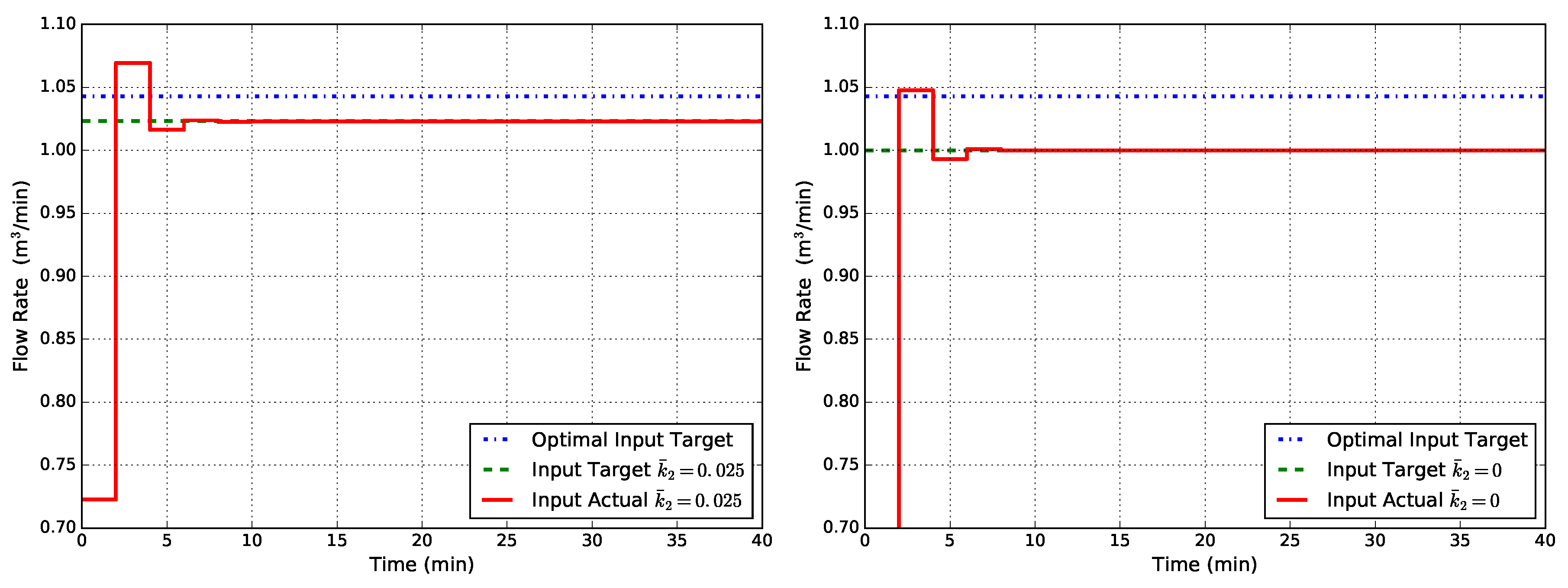
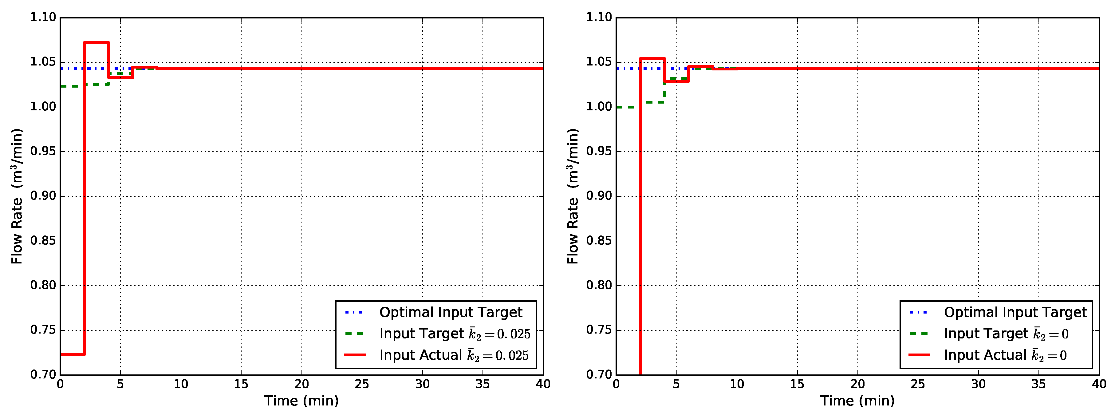
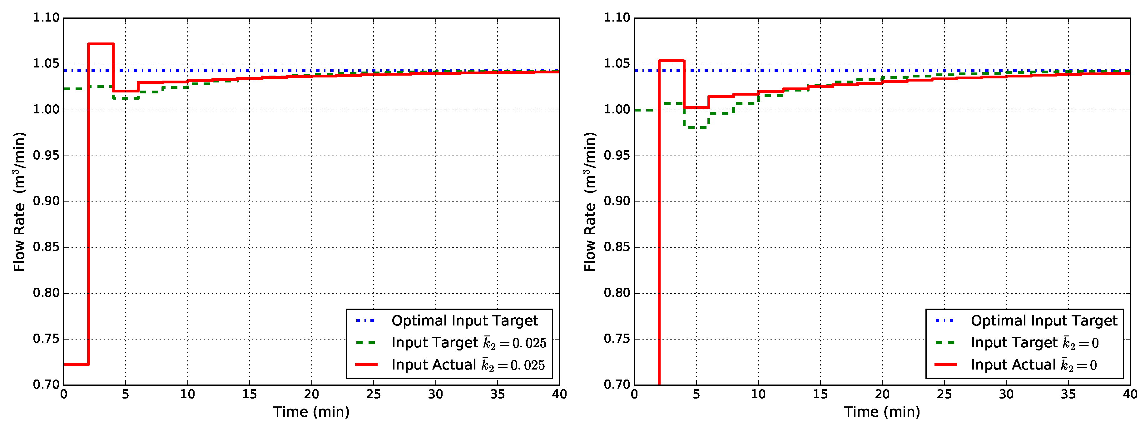
Figure 2 shows the closed-loop flow rate obtained with standard EMPC0 in two cases of uncertainty on $k_2$. In the first case (left), ${\overline{k}}_2=0.025$, i.e., the controller model uses a value of $k_2$, which is half of the true value. In the second case (right), ${\overline{k}}_2=0$, i.e., the controller model ignores the second reaction. As can be seen from these plots, in both cases, the controller is unable to drive the flow rate to the most economic target.

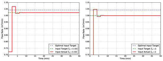
Figure 2. Closed-loop flow rate Q obtained with standard EMPC0 for two cases of uncertainty in $k_2$: ${\overline{k}}_2=0.025$ (left) and ${\overline{k}}_2=0$ (right).

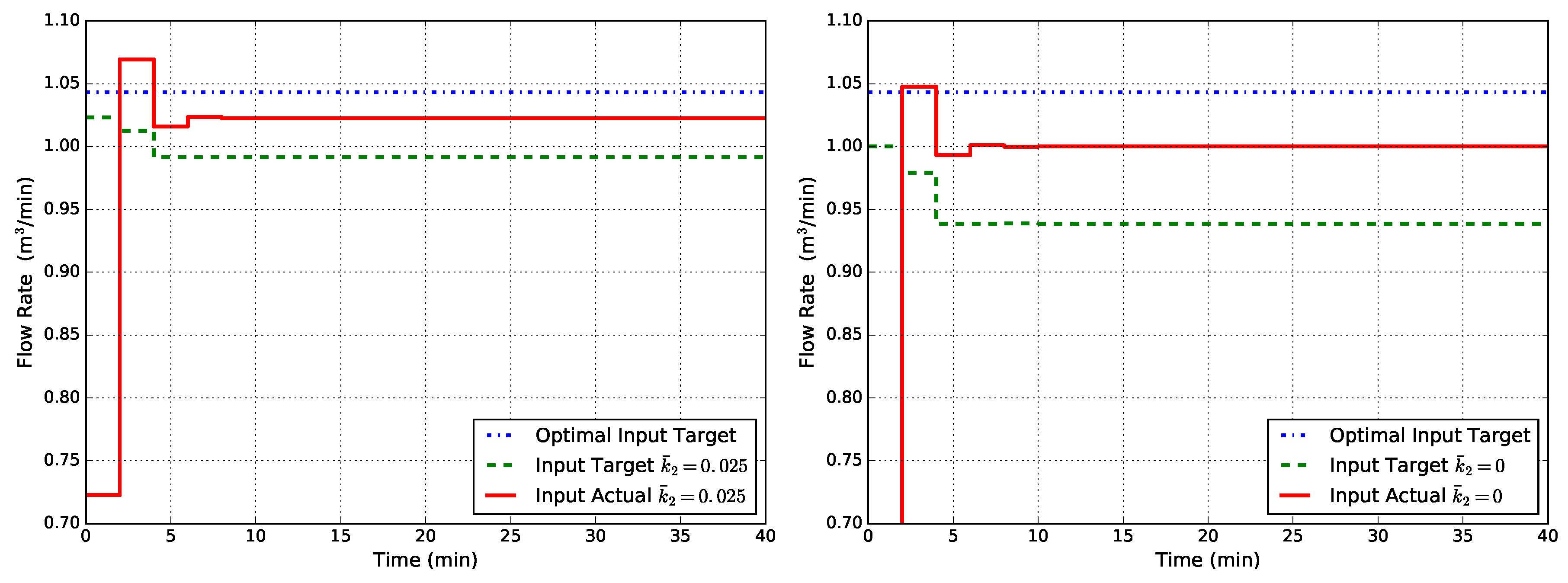
Figure 3 shows the corresponding results obtained with EMPC1. Despite the fact that EMPC1 uses a disturbance model, which guarantees offset-free tracking, the controller is still unable to drive the flow rate to the optimal target.

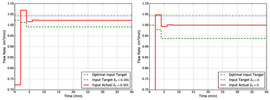
Figure 3. Closed-loop flow rate Q obtained with EMPC1 (state disturbance model) for two cases of uncertainty in $k_2$: ${\overline{k}}_2=0.025$ (left) and ${\overline{k}}_2=0$ (right).

Finally, Figure 4 shows the corresponding results obtained with EMPC2. In this case, the controller is able to drive the closed-loop system to the optimal steady state. The reason is that the augmented model (23) asymptotically converges to the true process because the estimated disturbance $d_2$ ensures that ${\overline{k}}_2+d_2\to k_2$. However, this approach requires to know exactly where the uncertainties are, in order to build an ad hoc disturbance model to correct them. Hence, it cannot be used as a general rule. With this evidence, it is clear that, at the moment, there is no general formulation for an offset-free economic MPC, and this is what motivates the present work. In the end, it has to be noted that the case ${\overline{k}}_2=0$ falls into an unmodeled dynamics problem, i.e., the second reaction is completely ignored by the model.

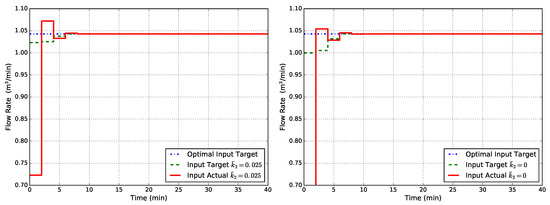
Figure 4. Closed-loop flow rate Q obtained with EMPC2 (non-linear state disturbance model) for two cases of uncertainty in $k_2$: ${\overline{k}}_2=0.025$ (left) and ${\overline{k}}_2=0$ (right).

3. Proposed Method

As introduced in the previous section, we now illustrate the method developed using the modifier-adaptation technique borrowed from the RTO literature. Before coming to the proposed method, we give a brief introduction to this technique, referring the interested reader to [14,16] for more details.

3.1. RTO with Modifier-Adaptation

The objective of RTO is the minimization of some steady-state operating cost function, while satisfying a number of constraints. Finding the optimal steady-state operation point for the actual process can be stated as the solution of the following problem:

$$\begin{array}{c}\underset{u}{min}{\mathrm{\Phi }}_p\left(u\right)\end{array}$$

(25a)

subject to

$$\begin{array}{c}\hfill C_p\left(u\right)\le 0\end{array}$$

(25b)

In the above, ${\mathrm{\Phi }}_p$: ${\mathbb{R}}^m\to \mathbb{R}$ is the economic performance cost function of the process and $C_p$: ${\mathbb{R}}^m\to {\mathbb{R}}^{n_c}$ is the process constraint function. As explained before for the MPC case, the exact process description is unknown, and only a model can be used in the process optimization. Hence, the model-based economic optimization is represented by the problem:

$$\begin{array}{c}\underset{u}{min}\mathrm{\Phi }(u,\theta )\end{array}$$

(26a)

subject to

$$\begin{array}{c}\hfill C(u,\theta )\le 0\end{array}$$

(26b)

where Φ: ${\mathbb{R}}^m\to \mathbb{R}$ and C: ${\mathbb{R}}^m\to {\mathbb{R}}^{n_c}$ represent the model economic cost function and the model constraint function, which may depend on uncertain parameters $\theta \in {\mathbb{R}}^{n_{\theta }}$. Due to plant-model mismatch, open-loop implementation of the solution to (26) may lead to suboptimal and even infeasible operation.

The modifier-adaptation methodology changes Problem (26) so that in a closed-loop execution, the necessary conditions of optimality (NCO) of the modified problem correspond to the necessary conditions of Process (25), upon convergence of the algorithm. The following problem shows the model-based optimization with additional modifiers [16,43]:

$$\begin{array}{c}{\overline{u}}_h=arg\underset{u}{min}{\mathrm{\Phi }}_M=\mathrm{\Phi }(u,\theta )+{\left({\lambda }_{h-1}^{\mathrm{\Phi }}\right)}^{T}u\end{array}$$

(27a)

subject to:

$$\begin{array}{c}\hfill C_M=C(u,\theta )+{\left({\lambda }_{h-1}^C\right)}^T(u-{\overline{u}}_{h-1})+{ϵ}_{h-1}^C\le 0\end{array}$$

(27b)

in which:

$$\begin{array}{c}{\lambda }_{h-1}^{\mathrm{\Phi }}={\nabla }_u{\mathrm{\Phi }}_p\left({\overline{u}}_{h-1}\right)-{\nabla }_u\mathrm{\Phi }({\overline{u}}_{h-1},\theta )\end{array}$$

(28a)

$$\begin{array}{c}{\lambda }_{h-1}^C={\nabla }_u{C}_p\left({\overline{u}}_{h-1}\right)-{\nabla }_{u}C({\overline{u}}_{h-1},\theta )\end{array}$$

(28b)

$$\begin{array}{c}{ϵ}_{h-1}^C=C_p\left({\overline{u}}_{h-1}\right)-C({\overline{u}}_{h-1},\theta )\end{array}$$

(28c)

In (27) and (28), ${\overline{u}}_{h-1}\in {\mathbb{R}}^m$ represents the operation point, calculated at the previous RTO iteration $h-1$, and the modifiers ${\lambda }_{h-1}^{\mathrm{\Phi }}\in {\mathbb{R}}^m$, ${\lambda }_{h-1}^C\in {\mathbb{R}}^{m\times n_c}$, and ${ϵ}_{h-1}^C\in {\mathbb{R}}^{n_c}$ are evaluated using the information available at that point. Notice that the model parameters θ are not updated.

Marchetti et al. [16,43] demonstrated that, upon convergence, the Karush–Kuhn–Tucker (KKT) conditions of the modified problem (27) match the ones of the true process optimization problem (25). Hence, if second-order conditions hold at this point, a local optimum of the real plant can be found by the problem modified as in (27). Furthermore, a filtering procedure of the modifiers is also recommended in order to improve stability and convergence and to reduce sensitivity to measurement noise. The filtering step is given by the following equations:

$$\begin{array}{c}{\lambda }_h^{\mathrm{\Phi }}=(I-K_{{\lambda }^{\mathrm{\Phi }}}){\lambda }_{h-1}^{\mathrm{\Phi }}+K_{{\lambda }^{\mathrm{\Phi }}}({\nabla }_u{\mathrm{\Phi }}_p\left({\overline{u}}_h\right)-{\nabla }_u\mathrm{\Phi }({\overline{u}}_h,\theta ))\end{array}$$

(29a)

$$\begin{array}{c}{\lambda }_h^C=(I-K_{{\lambda }^C}){\lambda }_{h-1}^C+K_{{\lambda }^C}({\nabla }_u{C}_p\left({\overline{u}}_h\right)-{\nabla }_{u}C({\overline{u}}_h,\theta ))\end{array}$$

(29b)

$$\begin{array}{c}{ϵ}_h^C=(I-K_{{ϵ}^C}){ϵ}_{h-1}^C+K_{{ϵ}^C}(C_p\left({\overline{u}}_h\right)-C({\overline{u}}_h,\theta ))\end{array}$$

(29c)

where $K_{{\lambda }^{\mathrm{\Phi }}}$, $K_{{\lambda }^C}$ and $K_{{ϵ}^C}$ (usually diagonal matrices) represent the respective first-order filter constants for each modifier. An alternative approach to the modifier filtering step (29) is to directly define the modifiers as the gradient or function differences and then filter the computed inputs to be applied to the process [44,45]. From (28) and (29), it is clear how the process gradient estimation stage is the major requirement of this method: actually, the process gradient estimation, is hidden into both ${\nabla }_u{\mathrm{\Phi }}_p$ and ${\nabla }_u{C}_p$ for calculating ${\lambda }_h^{\mathrm{\Phi }}$ and ${\lambda }_h^C$. This is also the major and tightest constraint for this method [46].

Before presenting the proposed technique, the example in Section 2.4 is tested on the standard hierarchical architecture RTO plus MPC. The RTO problem is modified as in Marchetti et al. [16] as follows:

$$\begin{array}{c}{\overline{u}}_h=arg\underset{u}{min}{\tilde{\mathrm{\Phi }}}_M=\mathrm{\Phi }(u,y(u,\theta )+{ϵ}_{h-1}^y+{({\lambda }_{h-1}^y)}^T(u-u_{h-1}))\end{array}$$

(30a)

subject to

$$\begin{array}{c}\hfill {\tilde{C}}_M=C(u,y(u,\theta )+{ϵ}_{h-1}^y+{\left({\lambda }_{h-1}^y\right)}^T(u-u_{h-1}))\le 0\end{array}$$

(30b)

where ${ϵ}_h^y$ and ${\lambda }_h^y$ are updated by the following law:

$$\begin{array}{c}{\lambda }_h^y=(I-K_{{\lambda }^y}){\lambda }_{h-1}^y+K_{{\lambda }^y}({\nabla }_u{y}_p\left({\overline{u}}_h\right)-{\nabla }_{u}y({\overline{u}}_h,\theta ))\end{array}$$

(31a)

$$\begin{array}{c}{ϵ}_h^y=(I-K_{{ϵ}^y}){ϵ}_{h-1}^y+K_{{ϵ}^y}(y_p\left({\overline{u}}_h\right)-y({\overline{u}}_h,\theta ))\end{array}$$

(31b)

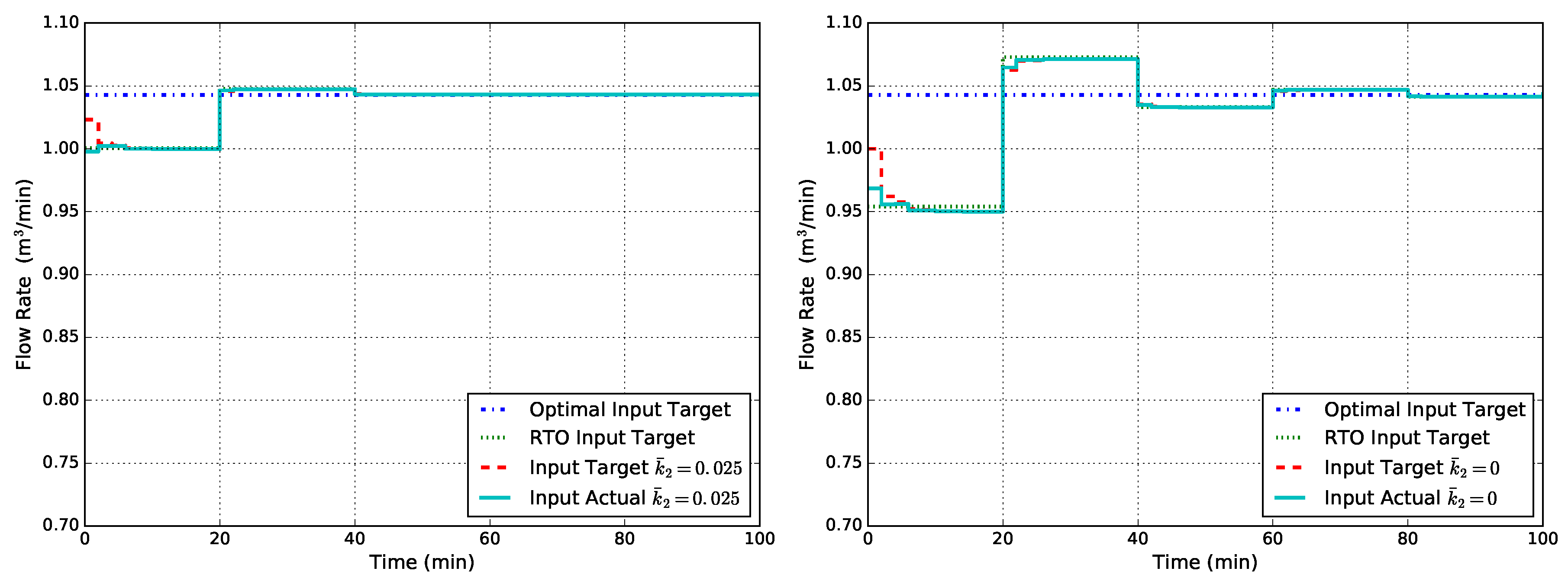
Figure 5 shows the closed-loop flow rate obtained with modified RTO problem followed by tracking MPC with output disturbance model in two cases of uncertainty on $k_2$. The weight values used are $K_{{\lambda }^y}=0.2$ and $K_{{ϵ}^y}=0.7$, and the RTO problem is run every 20 min. As can be seen from Figure 5, in both cases, the system achieves the optimal input value as expected by the modifier-adaptation methodology. However, the hierarchical and multi-rate nature of the standard architecture results in slow convergence towards the economically-optimal target.

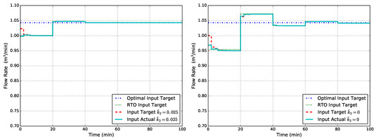
Figure 5. Closed-loop flow rate Q obtained with modified RTO followed by tracking MPC with the output disturbance model for two cases of uncertainty in $k_2$: ${\overline{k}}_2=0.025$ (left) and ${\overline{k}}_2=0$ (right).

3.2. Proposed Technique

Having shown that, in order to apply this technique to the EMPC, some work is needed. First of all, in order to be consistent with the offset-free augmented model and to exploit its properties, an alternative form of the modifier-adaptation technique is adopted. In this way, as illustrated in the work of Marchetti et al. [16], a linear modification of the model output steady-state function, rather than of the cost and constraint functions, independently, in the optimization problem has been preferred. To this aim, we rewrite the model constraints of the target problem (14) in a more compact form:

$$\left\{\begin{array}{c}{x}_s=F(x_s,{\widehat{d}}_{k|k},u_s)\\ y_s=H(x_s,{\widehat{d}}_{k|k})\end{array}\right.\Rightarrow y_s=G(u_s,{\widehat{d}}_{k|k})$$

(32)

in which G: ${\mathbb{R}}^{m+n_d}\to {\mathbb{R}}^p$. Then, the model output steady-state function is “artificially” modified as follows:

$$G_{\lambda }(u_s,{\widehat{d}}_{k|k})=G(u_s,{\widehat{d}}_{k|k})+{({\lambda }_{k-1}^G)}^T(u_s-u_{s,k-1})$$

(33)

where ${\lambda }_{k-1}^G\in {\mathbb{R}}^{m\times p}$ is a matrix to be defined later on and $u_{s,k-1}$ is the steady-state input target found at the previous sampling time, $k-1$. We observe that in [16], the modified output function also includes a zero order term, which ensures that $G_{\lambda }(·)\to G_p(·)$. However, such a term is unnecessary in the present framework because the model output convergence is already achieved by the offset-free augmented model formulation. Hence, only a gradient correction of G is necessary. In order to drive the target point towards the plant optimal value, we need to calculate ${\lambda }_{k-1}^G$ as a result of a KKT matching of the target optimization problem. In this way, similarly to what has been demonstrated in the RTO literature, the necessary condition of optimality can be satisfied.

The KKT matching is developed imposing the correspondence of the Lagrangian function gradient between the plant and model target optimization problems. The procedure is as follows.

Plant: Similarly to Model (32), a steady-state input-output map $y_{p,s}=G_p\left(u_s\right)$ can be defined also for the actual plant (1). In this way, the plant optimization steady-state problem reads:

$$\begin{array}{c}\underset{u}{min}{\ell }_e(G_p\left(u\right),u)\end{array}$$

(34a)

subject to:

$$\begin{array}{c}\hfill u_{min}\le u\le u_{max}\end{array}$$

(34b)

$$\begin{array}{c}\hfill y_{min}\le G_p\left(u\right)\le y_{max}\end{array}$$

(34c)

The Lagrangian function associated with Problem (34) is given by:

$$\begin{array}{c}\hfill {\mathcal{L}}_p(u,{\pi }_1,{\pi }_2,{\pi }_3,{\pi }_4)={\ell }_e(G_p\left(u\right),u)+{\pi }_1^T(u-u_{max})+{\pi }_2^T(u_{min}-u)+\end{array}$$

(35)

$$\begin{array}{c}\hfill {\pi }_3^T(G_p\left(u\right)-y_{max})+{\pi }_4^T(y_{min}-G_p\left(u\right)),\end{array}$$

(36)

then, the first-order necessary optimality KKT conditions for this problem are as follows. If $u^{\ast }$ is a (local) solution to (34), there exist vectors ${\pi }_1^{\ast },{\pi }_2^{\ast },{\pi }_3^{*},{\pi }_4^{\ast }$ satisfying the following conditions:

$$\begin{array}{cc}\hfill {\nabla }_u{\ell }_e(u^{\ast },G_p\left(u^{\ast }\right))+{\pi }_1^{\ast }-{\pi }_2^{\ast }+{\nabla }_u{G}_p\left(u^{\ast }\right){\pi }_3^{\ast }-{\nabla }_u{G}_p\left(u^{\ast }\right){\pi }_4^{\ast }& =0\hfill \end{array}$$

(37a)

$$\begin{array}{cc}\hfill u^{\ast }-u_{max}& \le 0\hfill \end{array}$$

(37b)

$$\begin{array}{cc}\hfill u_{min}-u^{\ast }& \le 0\hfill \end{array}$$

(37c)

$$\begin{array}{cc}\hfill G_p\left(u^{\ast }\right)-y_{max}& \le 0\hfill \end{array}$$

(37d)

$$\begin{array}{cc}\hfill y_{min}-G_p\left(u^{\ast }\right)& \le 0\hfill \end{array}$$

(37e)

$$\begin{array}{cc}\hfill {\pi }_1^{\ast },{\pi }_2^{\ast },{\pi }_3^{\ast },{\pi }_4^{\ast }& \ge 0\hfill \end{array}$$

(37f)

$$\begin{array}{cc}\hfill {(u^{\ast }-u_{max})}_j{\pi }_{1,j}^{\ast }=0& \hfill j=1,\dots ,m\end{array}$$

(37g)

$$\begin{array}{cc}\hfill {(u_{min}-u^{\ast })}_j{\pi }_{2,j}^{\ast }=0& \hfill j=1,\dots ,m\end{array}$$

(37h)

$$\begin{array}{cc}\hfill {(G_p\left(u^{\ast }\right)-y_{max})}_j{\pi }_{3,j}^{\ast }=0& \hfill j=1,\dots ,p\end{array}$$

(37i)

$$\begin{array}{cc}\hfill {(y_{min}-G_p\left(u^{\ast }\right))}_j{\pi }_{4,j}^{\ast }=0& \hfill j=1,\dots ,p.\end{array}$$

(37j)

in which ${\pi }_1,{\pi }_2\in {\mathbb{R}}^m$ are the multiplier vectors of the input bound constraints (34b), and ${\pi }_3,{\pi }_4\in {\mathbb{R}}^p$ are the multiplier vectors for output bound constraints (34c).

Model: With the modification introduced in (33), the model optimization steady-state problem can be rewritten as:

$$\begin{array}{c}\underset{u}{min}{\ell }_e(G_{\lambda }(u,{\widehat{d}}_{k|k}),u)\end{array}$$

(38a)

subject to:

$$\begin{array}{c}\hfill u_{min}\le u\le u_{max}\end{array}$$

(38b)

$$\begin{array}{c}\hfill y_{min}\le G_{\lambda }(u,{\widehat{d}}_{k|k})\le y_{max}\end{array}$$

(38c)

The Lagrangian function associated with (38) is given by:

$$\begin{array}{c}\hfill {\mathcal{L}}_m(u,{\pi }_1,{\pi }_2,{\pi }_3,{\pi }_4)={\ell }_e(G_{\lambda }(u,{\widehat{d}}_{k|k}),u)+{\pi }_1^T(u-u_{max})+{\pi }_2^T(u_{min}-u)+\end{array}$$

(39)

$$\begin{array}{c}\hfill {\pi }_3^T(G_{\lambda }(u,{\widehat{d}}_{k|k})-y_{max})+{\pi }_4^T(y_{min}-G_{\lambda }(u,{\widehat{d}}_{k|k})),\end{array}$$

(40)

then, the first-order necessary optimality KKT conditions for this problem are as follows. If $u^{\ast }$ is a (local) solution to (38), there exist vectors ${\pi }_1^{\ast },{\pi }_2^{\ast },{\pi }_3^{\ast },{\pi }_4^{\ast }$ satisfying the following:

$$\begin{array}{cc}\hfill {\nabla }_u{\ell }_e(G_{\lambda }(u^{\ast },{\widehat{d}}_{k|k}),u^{\ast })+{\pi }_1^{\ast }-{\pi }_2^{*}+{\nabla }_u{G}_{\lambda }(u^{\ast },{\widehat{d}}_{k|k}){\pi }_3^{\ast }-{\nabla }_u{G}_{\lambda }(u^{\ast },{\widehat{d}}_{k|k}){\pi }_4^{\ast }& =0\hfill \end{array}$$

(41a)

$$\begin{array}{cc}\hfill u^{\ast }-u_{max}& \le 0\hfill \end{array}$$

(41b)

$$\begin{array}{cc}\hfill u_{min}-u^{\ast }& \le 0\hfill \end{array}$$

(41c)

$$\begin{array}{cc}\hfill G_{\lambda }(u^{\ast },{\widehat{d}}_{k|k})-y_{max}& \le 0\hfill \end{array}$$

(41d)

$$\begin{array}{cc}\hfill y_{min}-G_{\lambda }(u^{\ast },{\widehat{d}}_{k|k})& \le 0\hfill \end{array}$$

(41e)

$$\begin{array}{cc}\hfill {\pi }_1^{\ast },{\pi }_2^{\ast },{\pi }_3^{\ast },{\pi }_4^{\ast }& \ge 0\hfill \end{array}$$

(41f)

$$\begin{array}{cc}\hfill {(u^{\ast }-u_{max})}_j{\pi }_{1,j}^{\ast }=0& \hfill j=1,\dots ,m\end{array}$$

(41g)

$$\begin{array}{cc}\hfill {(u_{min}-u^{\ast })}_j{\pi }_{2,j}^{\ast }=0& \hfill j=1,\dots ,m\end{array}$$

(41h)

$$\begin{array}{cc}\hfill {(G_{\lambda }(u^{\ast },{\widehat{d}}_{k|k})-y_{max})}_j{\pi }_{3,j}^{\ast }=0& \hfill j=1,\dots ,p\end{array}$$

(41i)

$$\begin{array}{cc}\hfill {(y_{min}-G_{\lambda }(u^{\ast },{\widehat{d}}_{k|k}))}_j{\pi }_{4,j}^{\ast }=0& \hfill j=1,\dots ,p.\end{array}$$

(41j)

KKT matching: To reach the KKT matching, conditions in (41) must converge to those in (37). We recall that, due to the offset-free augmented model, upon convergence, we have: $G(u^{\ast },{\widehat{d}}_{k|k})\to G_p(u^{\ast })$. Furthermore, upon convergence from (33), we also have: $G_{\lambda }(u^{\ast },{\widehat{d}}_{k|k})\to G(u^{\ast },{\widehat{d}}_{k|k})$ and therefore $G_{\lambda }(u^{\ast },{\widehat{d}}_{k|})\to G_p(u^{\ast })$. Therefore, in order for (41) to match (37), Conditions (37a) and (41a) have to be the same:

$${\nabla }_u{\mathcal{L}}_p(u^{\ast },{\pi }^{\ast })={\nabla }_u{\mathcal{L}}_m(u^{\ast },{\pi }^{\ast })$$

(42)

where

$${\pi }^{\ast }=[{\pi }_1^{\ast },{\pi }_2^{\ast },{\pi }_3^{\ast },{\pi }_4^{\ast }].$$

We expand the LHS and RHS in (42) to obtain:

$$\begin{array}{ccc}\hfill {\nabla }_u{\ell }_e(G_p\left(u^{\ast }\right),u^{\ast })& ={\left[\frac{\partial {\ell }_e(·,u^{\ast })}{\partial u}+\frac{\partial {\ell }_e(G_p(·),·)}{\partial G_p}\frac{\partial G_p\left(u^{\ast }\right)}{\partial u}\right]}^T\hfill & \hfill \mathrm{plant}\end{array}$$

(43)

$$\begin{array}{ccc}\hfill {\nabla }_u{\ell }_e(G_{\lambda }(u^{\ast },{\widehat{d}}_{k|k}),u^{\ast })& ={\left[\frac{\partial {\ell }_e(·,u^{\ast })}{\partial u}+\frac{\partial {\ell }_e(G_{\lambda }(·),·)}{\partial G_{\lambda }}\left[\frac{\partial G(u^{\ast },{\widehat{d}}_{k|k})}{\partial u}+{\left({\lambda }_{k-1}^G\right)}^T\right]\right]}^T\hfill & \hfill \mathrm{model}\end{array}$$

(44)

Then, the KKT matching condition is:

$$\frac{\partial G_p(u^{\ast })}{\partial u}=\frac{\partial G(u^{\ast },{\widehat{d}}_{k|k})}{\partial u}+{\left({\lambda }_{k-1}^G\right)}^T\Rightarrow {\left({\lambda }_{k-1}^G\right)}^T=\frac{\partial G_p(u^{\ast })}{\partial u}-\frac{\partial G(u^{\ast },{\widehat{d}}_{k|k})}{\partial u}$$

(45)

From (45), we also consider a filtering step and define the following update law for ${\lambda }_k^G$:

$${\lambda }_k^G=(1-{\alpha }_s){\lambda }_{k-1}^G+{\alpha }_s\left({\nabla }_u{G}_p\left(u_{s,k}\right)-{\nabla }_{u}G(u_{s,k},{\widehat{d}}_{k|k})\right)$$

(46)

where ${\alpha }_s$ is a scalar first-order filter constant, chosen in the range $(0,1]$. In order for the update law (46) to be applicable, we make the following assumption.

Assumption 2.

The gradient of the process steady-state input-output map $G_p(·)$ is known at steady-state points.

In general, the gradient of the process steady-state input-output map $G_p(·)$ can be (approximately) calculated through measurements of u and y [43,47,48,49]. We remark that the gradient of the model steady-state input-output map $G(·)$ instead can be computed from its definition (32) using the implicit function theorem. As a matter of fact, the gradient of $G(·)$ can be calculated as follows:

$${\nabla }_{u}G(·)={\nabla }_{x}H(x,d)\left[{\left(I-{\nabla }_{x}F(x,u,d)\right)}^{-1}{\nabla }_{u}F(x,u,d)\right]$$

(47)

Finally, from the above discussion, the following result is established.

Theorem 1.

KKT matching of the target optimization problem: Let the MPC target optimization problem be defined in (38), with ${\lambda }_k^G$ updated according to (46), and let $u_{s,k}$ be its solution at time k. Let the closed-loop system converge to an equilibrium, with $u_s^0:{lim}_{k\to \infty }{u}_{s,k}$ being the limit KKT point of the steady-state problem (38). Then, $u_s^0$ is also a KKT point for the plant optimization problem (34).

3.3. Summary

Summarizing, the offset-free economic MPC algorithm proposed in this work is the following. The estimation stage is taken from the offset-free tracking MPC as described in Section 2.2. Given the current state and disturbance estimate (${\widehat{x}}_{k|k},{\widehat{d}}_{k|k}$), the economic steady-state target problem is modified in this way:

$$\begin{array}{c}\underset{x,u,y}{min}{\ell }_e(y,u)\end{array}$$

(48a)

subject to

$$\begin{array}{c}\hfill x=F(x,{\widehat{d}}_{k|k},u)\end{array}$$

(48b)

$$\begin{array}{c}\hfill y=H(x,{\widehat{d}}_{k|k})+{\left({\lambda }_{k-1}^G\right)}^T(u-u_{s,k-1})\end{array}$$

(48c)

$$\begin{array}{c}\hfill u_{min}\le u\le u_{max}\end{array}$$

(48d)

$$\begin{array}{c}\hfill y_{min}\le y\le y_{max}\end{array}$$

(48e)

in which $u_{s,k-1}$ is the steady-state input target found at the previous sampling time $k-1$, and ${\lambda }_{k-1}^G$ is defined above in (46). Finally, the FHOCP solved at each time is the one defined in (15), unless differently specified in the next section.

4. Results and Discussion

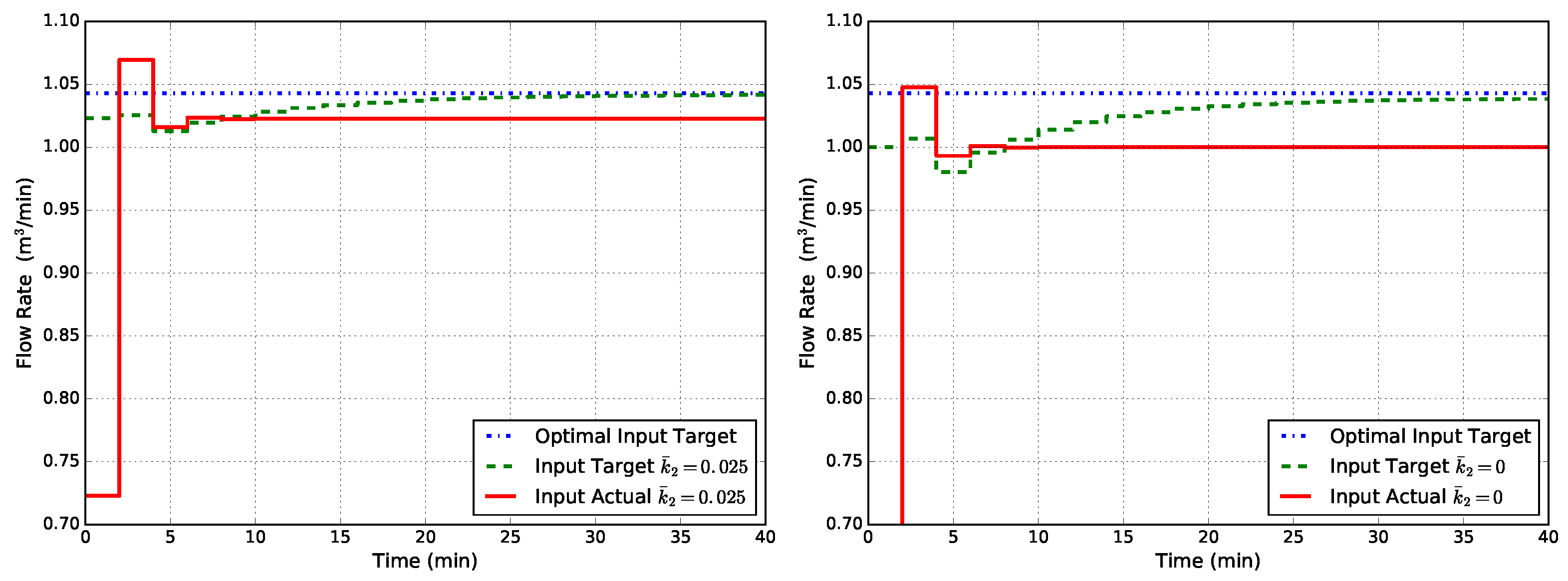
Simulation results of the proposed method applied to the reactor example illustrated in Section 2.4 are here reported. We use all simulation parameters defined in Section 2.4, and in addition, we set ${\alpha }_s=0.2$ for the modifiers update law (46). The first controller that is evaluated, named EMPC1-MT, uses the same augmented system with state disturbance model as EMPC1 and the same FHOCP formulation (15). The target problem instead is the modified one reported in (48). The obtained results are shown in Figure 6. As can be seen from Figure 6, the input target has asymptotically reached the optimal value (or it is very close to it in the case ${\overline{k}}_2=0$). The actual input value, instead, reaches an asymptotic value different from the optimal target. As a matter of fact, when the economic stage cost is used in the FHOCP (15), the offset still remains, and the EMPC formulation does not seem to have gained particular advantage from the target modification. This is also why for ${\overline{k}}_2=0$, the target does not reach perfectly the optimal value: as a recursive algorithm, it is obvious how the dynamic behavior also influences the steady-state target.

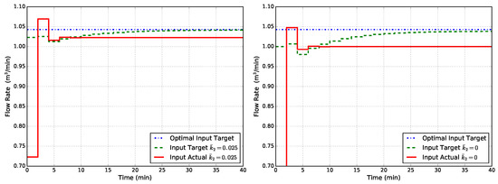
Figure 6. Closed-loop flow rate Q obtained with EMPC1-MT (state disturbance model, modified target problem) for two cases of uncertainty in $k_2$: ${\overline{k}}_2=0.025$ (left) and ${\overline{k}}_2=0$ (right).

We now consider another controller, named MPC1-MT, which is identical to EMPC1-MT, but uses a tracking stage cost in the FHOCP, i.e.,

$${\ell }_{QP}({\widehat{x}}_i,u_i)={({\widehat{x}}_i-x_{s,k})}^{T}Q({\widehat{x}}_i-x_{s,k})+{(u_i-u_{s,k})}^{T}R(u_i-u_{s,k})$$

(49)

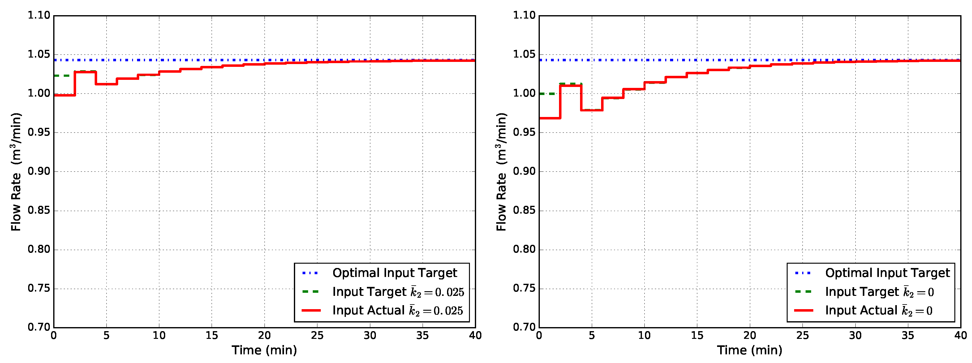
where $Q\in {\mathbb{R}}^{n\times n}$ and $R\in {\mathbb{R}}^{m\times m}$ are positive definite weight matrices. Results are shown in Figure 7, from which we observe that the offset is completely eliminated since both the input target and the actual input value go to the optimal one.The success of the tracking function can be explained by its design: the goal is to follow the steady-state target, and with the target suitably corrected, the actual value cannot go elsewhere in an offset-free formulation since the FHOCP cost function is positive definite around $(x_{s,k},u_{s,k})$.

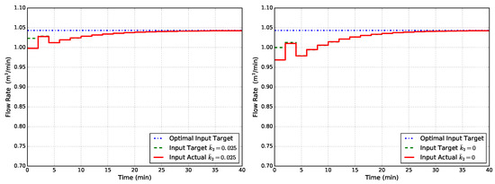
Figure 7. Closed-loop flow rate Q obtained with MPC1-MT (state disturbance model, modified target problem, tracking cost in the finite horizon optimal control problem (FHOCP)) for two cases of uncertainty in $k_2$: ${\overline{k}}_2=0.025$ (left) and ${\overline{k}}_2=0$ (right).

Despite the fact the MPC1-MT asymptotically reaches the optimal steady state, our primary goal is to build an offset-free economic MPC. Since now, the target problem has been adjusted by the modifier, results seem to suggest that a similar correction should be done for the FHOCP. Specifically, we consider the following modified FHOCP:

$$\begin{array}{c}\underset{\mathit{x},\mathit{u}}{min}\sum _{i=0}^{N-1}{\ell }_e(H(x_i,{\widehat{d}}_{k|k}),u_i)\end{array}$$

(50a)

subject to:

$$\begin{array}{c}\hfill x_0={\widehat{x}}_{k|k},\end{array}$$

(50b)

$$\begin{array}{c}\hfill x_{i+1}=F(x_i,u_i,{\widehat{d}}_{k|k})+{\mathrm{\Theta }}_{x,i}(x_i,u_i),i=0,\dots ,N-1\end{array}$$

(50c)

$$\begin{array}{c}\hfill u_{min}\le u_i\le u_{max},i=0,\dots ,N-1\end{array}$$

(50d)

$$\begin{array}{c}\hfill y_{min}\le H(x_i,{\widehat{d}}_{k|k})\le y_{max},i=0,\dots ,N-1\end{array}$$

(50e)

$$\begin{array}{c}\hfill x_N=x_{s,k}\end{array}$$

(50f)

where ${\mathrm{\Theta }}_{x,i}(x_i,u_i)\in {\mathbb{R}}^n$ is the correction term similar to ${\lambda }_{k-1}^G$ for the target module. A KKT matching performed on the FHOCP reveals that the required modification ${\mathrm{\Theta }}_{x,i}$ can be approximated as:

$${\mathrm{\Theta }}_{x,i}={\left({\lambda }_{k-1}^x\right)}^T(x_i-x_{s,k})+{\left({\lambda }_{k-1}^u\right)}^T(u_i-u_{s,k})$$

(51)

where:

$$\begin{array}{c}{\lambda }_k^x=(1-{\alpha }_x){\lambda }_{k-1}^x+{\alpha }_x\left({\nabla }_x{F}_p(x_{p,s,k},u_{s,k})-{\nabla }_{x}F(x_{s,k},u_{s,k},{\widehat{d}}_{k|k})\right)\end{array}$$

(52a)

$$\begin{array}{c}{\lambda }_k^u=(1-{\alpha }_u){\lambda }_{k-1}^u+{\alpha }_u\left({\nabla }_u{F}_p(x_{p,s,k},u_{s,k})-{\nabla }_{u}F(x_{s,k},u_{s,k},{\widehat{d}}_{k|k})\right)\end{array}$$

(52b)

and $x_{p,s,k}$ is the process state in equilibrium with $u_{s,k}$ according to (1). Having chosen constant values for ${\alpha }_x={\alpha }_u=0.1$, simulation results obtained with this controller, named EMPC1-MT-MD, are shown in Figure 8. From Figure 8, it can be seen that the offset has disappeared for both cases of uncertainty on the kinetic constant $k_2$.

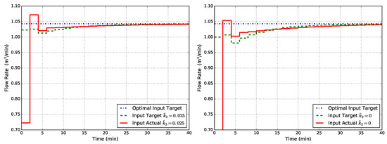
Figure 8. Closed-loop flow rate Q obtained with EMPC1-MT-MD (state disturbance model, modified target problem, modified FHOCP) for two cases of uncertainty in $k_2$: ${\overline{k}}_2=0.025$ (left) and ${\overline{k}}_2=0$ (right).

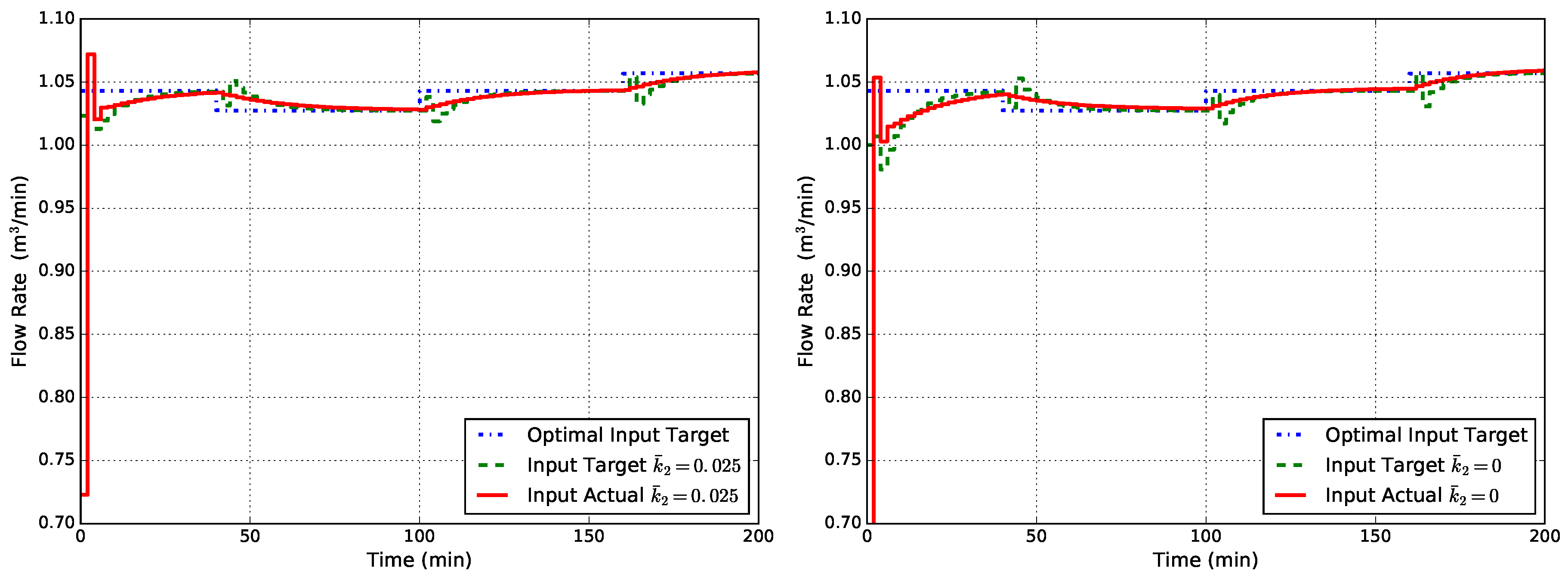
Furthermore, a time-varying simulation case is addressed, in which the true kinetic constant $k_2$ of the process is supposed to be varying during time following this step law:

$$k_2=\left\{\begin{array}{cc}0.05\hfill & \mathrm{if}0\le t<40\hfill \\ 0.03\hfill & \mathrm{if}40\le t<100\hfill \\ 0.05\hfill & \mathrm{if}100\le t<160\hfill \\ 0.07\hfill & \mathrm{if}160\le t<200\hfill \end{array}\right.$$

(53)

The controller used for this example is the one named EMPC1-MT-MD, and the reaction scheme it knows is still the one defined in (21) with the ${\overline{k}}_2$ value fixed. Simulation results obtained with this step time-varying disturbance in (53) are shown in Figure 9 where it can be seen that the offset has disappeared for both cases of uncertainty on the kinetic constant $k_2$.

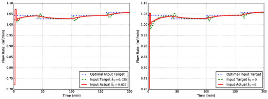
Figure 9. Closed-loop flow rate Q obtained with EMPC1-MT-MD (state disturbance model, modified target problem, modified FHOCP) for cases of unknown time-varying $k_2$: the MPC model uses a fixed value of ${\overline{k}}_2=0.025$ (left) and ${\overline{k}}_2=0.025$ (right).

In the end, it has to be noted that the majority of methods used for gradient estimation approximate the process gradient using a collection of previous output data to do a sort of identification [43,47,48,49]. Similarly, under the assumption that states are measured, i.e., $H_p\left(x\right)=x$, gradients ${\nabla }_x{F}_p(·)$ and ${\nabla }_u{F}_p(·)$ can be calculated if Assumption 2 holds true.

Further Comments

Currently, configurations that achieve optimal asymptotic operations are:

• EMPC2 (non-linear disturbance model). However, this is sort of an unfair choice. The disturbance has been positioned exactly where the uncertainties are, and this is cannot be considered as a general technique.
• MPC1-MT (economic modified target with tracking stage cost). This is the best general achievement at the moment and allows one to obtain offset-free economic performance for arbitrary plant-model mismatch.

As a matter of fact, it has to be underlined that, at the moment, the approximated modification term proposed in (51) works well in this example when there is no uncertainty on the first kinetic constant $k_1$. In other cases of uncertainty, the offset remains. Hence, further work has to be done to build a general correction strategy for the FHOCP with economic cost. Furthermore, assumptions made in this work deserve some comments. The strongest one is Assumption 2, which requires the availability of process steady-state gradients. For this purpose, we remark that gradient estimation is an active research area in the RTO literature (see, e.g., [19,43,50,51] and the references therein). Further work will investigate these approaches. In the end, it has to be noted that the proposed methodology does not add any computational burden compared to a conventional economic MPC algorithm. The modifiers can be updated after each optimization is concluded and inputs are sent to the plant, and the number of optimization variables is not augmented. Therefore, computation times are not affected.

5. Conclusions

In this paper, we addressed the problem of achieving the optimal asymptotic economic performance using the economic model predictive control (EMPC) algorithms despite the presence of plant-model mismatch.

After reviewing the standard techniques in offset-free tracking MPC and economic MPC, we presented an example where available MPC formulations fail in achieving the optimal asymptotic closed-loop performance. In order to eliminate this offset, the modifier-adaptation strategy developed in the real-time optimization (RTO) field has been taken into consideration and reviewed. Following this idea, a suitable correction to the target problem of the economic MPC algorithm has been formulated in order to achieve the necessary conditions of optimality despite the presence of plant/model mismatch. The proposed modification requires the availability of process gradients evaluated at the steady state. We then showed that the proposed modification is able to correct the steady-state target, but the actual closed-loop input may or may not converge to the optimal target depending on the finite horizon optimal control problem (FHOCP) stage cost. If such a cost is chosen to be positive definite around the target, as in tracking MPC, the optimal asymptotic behavior is achieved, although the dynamic performance may be suboptimal. For some cases of uncertainty, we showed that an economic stage cost can still be used by introducing a modification to the FHOCP.

Finally, we should remark about the main limitations of the current method and suggest future developments. First of all, the availability of process gradients should be reconsidered and relaxed as much as possible. Then, a general correction strategy for using an economic stage cost in the FHOCP, while enforcing convergence to the targets, has to be obtained.

References

- Qin, S.J.; Badgwell, T.A. A survey of industrial model predictive control technology. Control Eng. Pract. 2003, 11, 733–764. [Google Scholar] [CrossRef]
- Engell, S. Feedback control for optimal process operation. J. Process Control 2007, 17, 203–219. [Google Scholar] [CrossRef]
- Guay, M.; Zhang, T. Adaptive extremum seeking control of nonlinear dynamic systems with parametric uncertainties. Automatica 2003, 39, 1283–1293. [Google Scholar] [CrossRef]
- Guay, M.; Peters, N. Real-time dynamic optimization of nonlinear systems: A flatness-based approach. Comput. Chem. Eng. 2006, 30, 709–721. [Google Scholar] [CrossRef]
- Muske, K.R.; Badgwell, T.A. Disturbance modeling for offset-free linear model predictive control. J. Process Control 2002, 12, 617–632. [Google Scholar] [CrossRef]
- Pannocchia, G.; Rawlings, J.B. Disturbance models for offset-free model-predictive control. AIChE J. 2003, 49, 426–437. [Google Scholar] [CrossRef]
- Pannocchia, G. Offset-free tracking MPC: A tutorial review and comparison of different formulations. In Proceedings of the 2015 European Control Conference (ECC), Linz, Austria, 15–17 July 2015; pp. 527–532.
- Marlin, T.E.; Hrymak, A.N. Real-time operations optimization of continuous processes. AIChE Sympos. Ser. 1997, 93, 156–164. [Google Scholar]
- Chen, C.Y.; Joseph, B. On-line optimization using a two-phase approach: An application study. Ind. Eng. Chem. Res. 1987, 26, 1924–1930. [Google Scholar] [CrossRef]
- Garcia, C.E.; Morari, M. Optimal operation of integrated processing systems: Part II: Closed-loop on-line optimizing control. AIChE J. 1984, 30, 226–234. [Google Scholar] [CrossRef]
- Skogestad, S. Self-optimizing control: The missing link between steady-state optimization and control. Comput. Chem. Eng. 2000, 24, 569–575. [Google Scholar] [CrossRef]
- François, G.; Srinivasan, B.; Bonvin, D. Use of measurements for enforcing the necessary conditions of optimality in the presence of constraints and uncertainty. J. Process Control 2005, 15, 701–712. [Google Scholar] [CrossRef]
- Forbes, J.F.; Marlin, T.E. Model accuracy for economic optimizing controllers: The bias update case. Ind. Eng. Chem. Res. 1994, 33, 1919–1929. [Google Scholar] [CrossRef]
- Chachuat, B.; Marchetti, A.G.; Bonvin, D. Process optimization via constraints adaptation. J. Process Control 2008, 18, 244–257. [Google Scholar] [CrossRef]
- Chachuat, B.; Srinivasan, B.; Bonvin, D. Adaptation strategies for real-time optimization. Comput. Chem. Eng. 2009, 33, 1557–1567. [Google Scholar] [CrossRef]
- Marchetti, A.G.; Chachuat, B.; Bonvin, D. Modifier-adaptation methodology for real-time optimization. Ind. Eng. Chem. Res. 2009, 48, 6022–6033. [Google Scholar] [CrossRef]
- Alvarez, L.A.; Odloak, D. Robust integration of real time optimization with linear model predictive control. Comput. Chem. Eng. 2010, 34, 1937–1944. [Google Scholar] [CrossRef]
- Alvarez, L.A.; Odloak, D. Optimization and control of a continuous polymerization reactor. Braz. J. Chem. Eng. 2012, 29, 807–820. [Google Scholar] [CrossRef]
- Marchetti, A.G.; Luppi, P.; Basualdo, M. Real-time optimization via modifier adaptation integrated with model predictive control. IFAC Proc. Vol. 2011, 44, 9856–9861. [Google Scholar] [CrossRef]
- Marchetti, A.G.; Ferramosca, A.; González, A.H. Steady-state target optimization designs for integrating real-time optimization and model predictive control. J. Process Control 2014, 24, 129–145. [Google Scholar] [CrossRef]
- Kadam, J.V.; Schlegel, M.; Marquardt, W.; Tousain, R.L.; van Hessem, D.H.; van Den Berg, J.H.; Bosgra, O.H. A two-level strategy of integrated dynamic optimization and control of industrial processes—A case study. Comput. Aided Chem. Eng. 2002, 10, 511–516. [Google Scholar]
- Kadam, J.; Marquardt, W.; Schlegel, M.; Backx, T.; Bosgra, O.; Brouwer, P.; Dünnebier, G.; Van Hessem, D.; Tiagounov, A.; De Wolf, S. Towards integrated dynamic real-time optimization and control of industrial processes. In Proceedings of the Foundations of Computer-Aided Process Operations (FOCAPO2003), Coral Springs, FL, USA, 12–15 January 2003; pp. 593–596.
- Kadam, J.V.; Marquardt, W. Integration of economical optimization and control for intentionally transient process operation. In Assessment and Future Directions of Nonlinear Model Predictive Control; Springer: Berlin/Heidelberg, Germany, 2007; pp. 419–434. [Google Scholar]
- Biegler, L.T. Technology advances for dynamic real-time optimization. Comput. Aided Chem. Eng. 2009, 27, 1–6. [Google Scholar]
- Gopalakrishnan, A.; Biegler, L.T. Economic nonlinear model predictive control for periodic optimal operation of gas pipeline networks. Comput. Chem. Eng. 2013, 52, 90–99. [Google Scholar] [CrossRef]
- Maeder, U.; Borrelli, F.; Morari, M. Linear offset-free model predictive control. Automatica 2009, 45, 2214–2222. [Google Scholar] [CrossRef]
- Morari, M.; Maeder, U. Nonlinear offset-free model predictive control. Automatica 2012, 48, 2059–2067. [Google Scholar] [CrossRef]
- Rawlings, J.B.; Mayne, D.Q. Model Predictive Control: Theory and Design; Nob Hill Pub.: San Francisco, CA, USA, 2009. [Google Scholar]
- Pannocchia, G.; Gabiccini, M.; Artoni, A. Offset-free MPC explained: Novelties, subtleties, and applications. IFAC-PapersOnLine 2015, 48, 342–351. [Google Scholar] [CrossRef]
- Würth, L.; Hannemann, R.; Marquardt, W. A two-layer architecture for economically optimal process control and operation. J. Process Control 2011, 21, 311–321. [Google Scholar] [CrossRef]
- Zhu, X.; Hong, W.; Wang, S. Implementation of advanced control for a heat-integrated distillation column system. In Proceedings of the 30th Annual Conference of IEEE Industrial Electronics Society (IECON), Busan, Korea, 2–6 November 2004; Volume 3, pp. 2006–2011.
- Rawlings, J.B.; Angeli, D.; Bates, C.N. Fundamentals of economic model predictive control. In Proceedings of the 51st IEEE Conference on Decision and Control (CDC), Maui, HI, USA, 10–13 December 2012; pp. 3851–3861.
- Angeli, D.; Amrit, R.; Rawlings, J.B. Receding horizon cost optimization for overly constrained nonlinear plants. In Proceedings of the 48th IEEE Conference on Decision and Control (CDC), Shanghai, China, 15–18 December 2009; pp. 7972–7977.
- Heidarinejad, M.; Liu, J.; Christofides, P.D. Economic model predictive control of nonlinear process systems using Lyapunov techniques. AIChE J. 2012, 58, 855–870. [Google Scholar] [CrossRef]
- Ellis, M.; Christofides, P.D. On finite-time and infinite-time cost improvement of economic model predictive control for nonlinear systems. Automatica 2014, 50, 2561–2569. [Google Scholar] [CrossRef]
- Angeli, D.; Amrit, R.; Rawlings, J.B. On average performance and stability of economic model predictive control. IEEE Trans. Autom. Control 2012, 57, 1615–1626. [Google Scholar] [CrossRef]
- Faulwasser, T.; Bonvin, D. On the design of economic NMPC based on an exact turnpike property. IFAC-PapersOnLine 2015, 48, 525–530. [Google Scholar] [CrossRef]
- Faulwasser, T.; Bonvin, D. On the design of economic NMPC based on approximate turnpike properties. In Proceedings of the 54th IEEE Conference on Decision and Control (CDC), Osaka, Japan, 15–18 December 2015; pp. 4964–4970.
- Faulwasser, T.; Korda, M.; Jones, C.N.; Bonvin, D. Turnpike and dissipativity properties in dynamic real-time optimization and economic MPC. In Proceedings of the 53rd IEEE Conference on Decision and Control, Los Angeles, CA, USA, 15–17 December 2014; pp. 2734–2739.
- Faulwasser, T.; Korda, M.; Jones, C.N.; Bonvin, D. On Turnpike and Dissipativity Properties of Continuous-Time Optimal Control Problems. arXiv preprint arXiv:1509.07315, 2015; arXiv:1509.07315. [Google Scholar]
- Ellis, M.; Durand, H.; Christofides, P.D. A tutorial review of economic model predictive control methods. J. Process Control 2014, 24, 1156–1178. [Google Scholar] [CrossRef]
- Ellis, M.; Liu, J.; Christofides, P.D. Economic Model Predictive Control: Theory, Formulations and Chemical Process Applications; Springer: Berlin/Heidelberg, Germany, 2016. [Google Scholar]
- Marchetti, A.G.; Chachuat, B.; Bonvin, D. A dual modifier-adaptation approach for real-time optimization. J. Process Control 2010, 20, 1027–1037. [Google Scholar] [CrossRef]
- Brdys, M.A.; Tatjewski, P. Iterative Algorithms for Multilayer Optimizing Control; World Scientific: London, UK, 2005. [Google Scholar]
- Bunin, G.A.; François, G.; Srinivasan, B.; Bonvin, D. Input filter design for feasibility in constraint-adaptation schemes. IFAC Proc. Vol. 2011, 44, 5585–5590. [Google Scholar] [CrossRef]
- Navia, D.; Briceño, L.; Gutiérrez, G.; De Prada, C. Modifier-adaptation methodology for real-time optimization reformulated as a nested optimization problem. Ind. Eng. Chem. Res. 2015, 54, 12054–12071. [Google Scholar] [CrossRef]
- Bunin, G.A.; François, G.; Bonvin, D. Exploiting local quasiconvexity for gradient estimation in modifier-adaptation schemes. In Proceedings of the 2012 American Control Conference (ACC), Montreal, QC, Canada, 27–29 June 2012; pp. 2806–2811.
- Serralunga, F.J.; Mussati, M.C.; Aguirre, P.A. Model adaptation for real-time optimization in energy systems. Ind. Eng. Chem. Res. 2013, 52, 16795–16810. [Google Scholar] [CrossRef]
- Gao, W.; Wenzel, S.; Engell, S. Modifier adaptation with quadratic approximation in iterative optimizing control. In Proceedings of the IEEE 2015 European Control Conference (ECC), Linz, Austria, 15–17 July 2015; pp. 2527–2532.
- Brdys, M.A.; Tatjewski, P. An algorithm for steady-state optimising dual control of uncertain plants. In Proceedings of the IFAC Workshop on New Trends in Design of Control Systems, Smolenice, Slovak, 7–10 September 1994; pp. 249–254.
- Costello, S.; François, G.; Bonvin, D. A directional modifier-adaptation algorithm for real-time optimization. J. Process Control 2016, 39, 64–76. [Google Scholar] [CrossRef]
© 2016 by the authors. Licensee MDPI, Basel, Switzerland. This article is an open access article distributed under the terms and conditions of the Creative Commons Attribution (CC BY) license ( http://creativecommons.org/licenses/by/4.0/).