Impact of Sensor Network Resolution on Methane Leak Characterization in Large Indoor Spaces for Green-Fuel Vessel Applications

Abstract

A quantitative understanding of methane leakage has become essential for safety design as eco-friendly fuel systems expand in modern ship applications. To address this need, controlled methane-release experiments were conducted in a large indoor chamber (30 × 16 × 20 m) to evaluate how sensor-network resolution (1 m vs. 0.5 m spacing) influences dispersion measurement and 5% Lower Explosive Limit (LEL)-based risk assessment. Initial tests with a 1 m grid showed that most sensors detected only low concentrations except for near the release nozzle, demonstrating that coarse spatial resolution cannot capture the primary dispersion pathway or transient peaks. This limitation motivated the use of a 0.5 m high-density sensor network, which enabled clear identification of the dispersion centerline, concentration-gradient development, early detection behavior, and the evolution of diluted regions, particularly under buoyancy-driven plume rise. Experimental results were compared with CFD simulations using the RNG k–ε and k–ω GEKO turbulence models. Strong agreement was obtained in peak concentration, concentration-rise rates during the accumulation phase, and LEL-based dispersion distances. These findings confirm the suitability of the selected turbulence models for predicting methane behavior in large enclosed spaces and highlight the sensitivity of model–experiment agreement to measurement resolution. The results provide an experimentally grounded reference for sensor layout design and verification of gas-detection strategies in ship compartments, fuel-gas preparation rooms, and modular supply units. Overall, the study establishes a methodological framework that integrates high-resolution experiments with CFD modeling to support safer design and operation of methane-fueled vessels.

1. Introduction

1.1. Background and Motivation

Methane, the primary constituent of liquefied natural gas (LNG), has emerged as a central alternative fuel within the maritime sector’s strategy for decarbonization and compliance with increasingly stringent environmental regulations. The IMO’s 2020 sulfur cap, combined with its long-term greenhouse-gas reduction objectives for 2030 and 2050, has motivated shipping companies worldwide to accelerate the adoption of LNG-fueled vessels. Compared with conventional heavy fuel oil, LNG enables substantial reductions in sulfur oxide, nitrogen oxide, particulate matter, and carbon dioxide emissions. As a result, the proportion of newly ordered vessels equipped with LNG propulsion has continued to rise, and LNG is now considered a transitional yet pivotal fuel in the shift toward greener shipping.

Despite these advantages, methane poses significant safety challenges due to its low Lower Explosive Limit (LEL, approximately 5 vol%) and its density, which is lower than that of air. When leakage occurs, methane tends to rise and accumulate in overhead regions, particularly in enclosed or semi-enclosed shipboard environments. Engine rooms, fuel-gas supply and preparation modules, machinery spaces, and the upper void of cargo holds often feature restricted ventilation pathways and structurally complex geometries. Under these conditions, localized pockets of elevated concentration can develop rapidly, greatly increasing the likelihood of ignition and explosion. Numerous incidents across both the marine industry and onshore gas-processing facilities highlight how even minor leaks, if undetected, can escalate into severe accidents.

To mitigate such risks, the IMO requires vessels using low-flashpoint fuels to be equipped with gas-detection systems through the IGF Code and IGC Code. Classification societies further provide guidelines concerning installation height, sensor density, detection limits, and performance requirements. However, these recommendations are largely derived from empirical safety margins or simplified ventilation assumptions. They frequently do not incorporate detailed knowledge of transient dispersion behavior in large, three-dimensional spaces, especially where ventilation patterns are non-uniform or obstructed by machinery and structural members. Consequently, the effectiveness of sensor placement strategies can vary widely, and the probability of missing early-stage accumulation zones remains non-negligible.

For these reasons, a high-fidelity understanding of methane dispersion characteristics—supported by controlled experiments and advanced numerical modeling—is essential for improving the design of gas-detection networks. Such an understanding is not only crucial for LNG-fueled ships but will also play a foundational role in future vessels powered by next-generation alternative fuels, such as hydrogen and ammonia, which present similar or even greater challenges in terms of leak behavior and explosion risk. In particular, the spatial resolution of the sensor network strongly influences the ability to capture concentration gradients, detect early LEL-approaching regions, and characterize the dynamic evolution of dispersion plumes. Therefore, a systematic investigation into how sensor spacing and density affect detectability, accuracy, and risk assessment is both timely and necessary for establishing reliable safety standards.

1.2. Research Objectives and Scope

The primary objective of this study is to measure methane dispersion behavior in a large-scale enclosed space and to quantitatively evaluate the influence of sensor-network resolution. For this purpose, a large indoor chamber measuring 30 m in length, 16 m in width, and 20 m in height was constructed, and two different sensor networks—with spacings of 1 m and 0.5 m—were deployed. Initial experiments using the 1 m network revealed limitations, as high concentrations were detected only near the nozzle while most sensors recorded low concentrations below 2–3%. To address this issue, the sensor spacing was reduced to 0.5 m and the sensor layout was partially reconfigured. In this study, this refined configuration is referred to as a ‘high-resolution’ sensor network in a relative sense, specifically in comparison with the preliminary 1 m spacing network, enabling enhanced capture of fine-scale concentration variations along the dispersion pathway.

The scope of this research is defined through the three components described below.

(1)

Assessment of sensor-network resolution effects: By comparing concentration capture, concentration gradients, and LEL detectability between the 1 m and 0.5 m networks, the sensitivity of sensor-placement strategies is evaluated.

(2)

Experimental–numerical comparison and validation: CFD simulations are performed based on the experimental data, and key metrics—including peak concentration at each sensor location, time lag, and concentration rise rate—are compared to validate the numerical model. In this study, four high-quality test cases obtained from the 0.5 m network were selected for simulation.

(3)

Practical applicability: The findings are used to propose evidence-based guidelines for optimizing gas-detector placement in real shipboard environments, such as LNG-fueled vessel compartments, with potential extension to next-generation alternative-fuel ships using hydrogen or ammonia.

The objective of this study is to investigate methane dispersion behavior in a large enclosed space with a specific focus on the influence of sensor-network resolution on concentration measurement and experimental–numerical validation. Rather than reproducing a particular ship engine-room configuration, a controlled baseline approach is adopted to ensure experimental–numerical comparability and parameter isolation. Among the many factors affecting gas dispersion, only variables that can be systematically controlled in large-scale experiments and consistently reproduced in CFD simulations are varied. In this framework, the volumetric release rate represents the release intensity, while sensor-network resolution is treated as the primary measurement-related parameter. Other factors, such as nozzle geometry, orientation, and ventilation, are intentionally fixed or excluded to avoid overlapping physical effects that would obscure the independent role of sensor resolution. The resulting dataset is intended to provide reference dispersion characteristics under well-defined conditions, serving as a baseline for future studies incorporating additional physical complexity.

1.3. Review of Previous Studies

Research on gas dispersion has been conducted through a wide range of approaches, including small-scale experiments, CFD-based analyses, optimization of detector placement, and data-driven modeling. Experimental studies have been reported in which gas leakage through soil layers was reproduced using buried pipelines, and the resulting dispersion behavior was used to validate CFD models [1]. Although these studies provided valuable insight into early-stage leakage behavior, their applicability to large, complex enclosed spaces is limited due to the simplified soil–pipeline configuration. Other studies have examined flammable-gas accumulation and ignition potential in small-scale chambers to propose safety criteria [2], but the restricted experimental scale makes it difficult to generalize the findings to large compartments or shipboard environments.

A substantial body of numerical research has also been published. CFD analyses have been performed to evaluate methane dispersion resulting from pipeline damage in geometrically complex compartments, assessing the formation of localized high-concentration regions and the potential for reaching LEL conditions [3]. However, these studies were constrained by limited experimental data, leaving uncertainties in the validation of the numerical models. Three-dimensional CFD investigations incorporating building geometry and ambient airflow have been conducted for urban pipeline leakage scenarios [4], but such approaches are better suited to outdoor environments and are not directly applicable to concentration distributions inside enclosed volumes. Other studies have examined multi-gas dispersion and various leakage configurations under steady and transient conditions [5], yet the lack of direct comparison with experimental data restricts their ability to establish model reliability. Methane monitoring strategies and classification frameworks have been established to guide the selection and evaluation of measurement methods and sensor configurations in various application contexts [6]. Nonetheless, the absence of validation using large-scale experimental data raises questions about the practical applicability of the proposed placement strategies. Risk-based simulation approaches have also been used to suggest optimal sensor locations in industrial plants [7], but these remain heavily model-dependent and are difficult to apply directly to complex, confined compartments found on ships.

More recently, data-driven methods have been investigated. Deep-learning-based CFD surrogate models have been developed to estimate leak-source location and release intensity in real time [8]. While these approaches offer advantages in computational efficiency, their performance strongly depends on the range and quality of the training dataset, and their consistency with large-scale experimental observations has not yet been fully demonstrated.

Computational fluid dynamics (CFD) has been widely established as a versatile and reliable analysis tool across a broad range of engineering and scientific applications, extending beyond conventional fluid transport problems to areas such as complex coupled transport systems and biomedical flows [9,10,11,12,13]. Owing to its ability to resolve detailed flow and dispersion characteristics under controlled and practical conditions, CFD has become an essential framework for analyzing transport phenomena where experimental access is limited or incomplete.

Within this broader context, previous studies on gas dispersion have made meaningful progress through small-scale experiments, numerical simulations, detector-placement optimization, and data-driven modeling. However, very few studies have systematically examined the influence of sensor-network resolution on dispersion measurement in large enclosed spaces through integrated experiment–CFD comparisons. In particular, experimental investigations conducted at chamber scales comparable to real ship compartments—on the order of tens of meters—and their direct use for numerical model validation remain extremely limited. The present study aims to address this gap by establishing a rigorous connection between large-scale experimental measurements and predictive numerical modeling.

Beyond enclosed and shipboard environments, extensive research has been conducted on methane sensing networks for outdoor oil and gas infrastructure and environmental monitoring applications. These studies include fixed and mobile sensor deployments along pipelines and production facilities, large-area monitoring strategies, and inverse modeling approaches for source localization and emission quantification [14,15,16]. While these outdoor-focused studies have provided valuable insight into large-scale monitoring efficiency and network optimization, their direct applicability to large enclosed spaces is limited due to fundamentally different dispersion regimes. In open or semi-open environments, dispersion behavior is dominated by atmospheric turbulence, wind-driven advection, and surface roughness, whereas methane leakage in enclosed compartments is governed primarily by buoyancy-driven rise, confinement effects, and restricted ventilation. Accordingly, the present study does not attempt to transfer outdoor sensor-placement methodologies directly to enclosed shipboard environments, but rather complements existing outdoor methane monitoring research by providing experimentally validated insight into sensor-network resolution requirements under buoyancy-dominated dispersion in large enclosed volumes relevant to maritime applications.

2. Methodology

The methodology of this study consists of two major components: an experimental approach and a numerical (CFD) approach. First, methane leakage was simulated in a large chamber, and concentration distributions were measured under different sensor-network configurations to obtain experimental data. Subsequently, CFD simulations were conducted under the same conditions, and the numerical results were compared and validated against the experimental measurements. This dual approach enables direct quantification of actual dispersion behavior through experiments, while numerical analysis provides a predictive framework that can be extended to a broader range of conditions.

2.1. Experimental Methodology

2.1.1. Overview of the Experiment

The aim of the experimental component is to investigate how the spatial resolution of a sensor network influences the measurement of methane concentration distribution in a large enclosed space, and to evaluate the consistency between high-resolution sensor-based observations, dispersion characteristics, and CFD predictions. To achieve this, two sequential sensor-network configurations were employed, as illustrated in Figure 1.

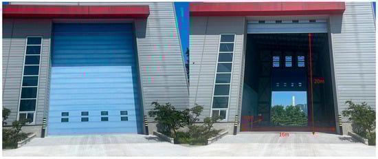
Figure 1. Large-scale enclosed chamber used for methane dispersion experiments (30 × 16 × 20 m).

In the preliminary stage, a low-resolution network with approximately 1 m spacing was deployed to examine dispersion behavior under representative flow-rate conditions (240 LPM and 600 LPM). The preliminary tests confirmed that sensor placement and resolution play a critical role in identifying the dispersion centerline and concentration gradients. Based on these findings, the final experimental campaign adopted a high-resolution sensor network with 0.5 m spacing.

In the main experiment, four flow-rate conditions ranging from 240 to 600 LPM were evaluated. The configurations of the sensor networks and the detailed test conditions are summarized in Table 1 and Table 2.

Table 1. Methane leak scenarios for low-resolution sensor network (1 m spacing).

Case	Nozzle Dia. (mm)	Gas Type	Flow Rate (LPM)	Leak Time (s)	Measurement Points
1	25	LNG (CH4)	240	≥30	8 points *
2	25	LNG (CH4)	600	≥30	8 points *

Table 2. Methane leak scenarios for high-resolution sensor network (0.5 m spacing).

Case	Nozzle Dia. (mm)	Gas Type	Flow Rate (LPM)	Leak Time (s)	Measurement Points
1	25	LNG (CH4)	240	≥30	8 points †
2	25	LNG (CH4)	360	≥30	8 points †
3	25	LNG (CH4)	480	≥30	8 points †
4	25	LNG (CH4)	600	≥30	8 points †

2.1.2. Test Gas and Experimental Apparatus

Industrial-grade methane (Grade 2, approximately 99% purity) was used as the test gas. This grade has been widely employed in previous hydrate experiments and gas-dispersion studies and provides sufficient accuracy for evaluating relative concentrations relevant to explosion-safety assessments [16]. The flow rate was controlled using a mass flow controller (MFC) with a specified accuracy of ±1% full scale (FS), according to the manufacturer’s specifications and in accordance with ISO 6145-7 [17].

As shown in Figure 2, the leakage nozzle was fabricated as a circular opening with a diameter of 25 mm and installed horizontally at a height of 0.5 m above the floor. This configuration represents a simplified and well-controlled release geometry that is suitable for observing buoyancy-driven dispersion behavior of methane in confined spaces [18].

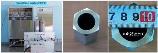
Figure 2. Gas supply system and nozzle (Ø 25 mm) used in this experiment.

2.1.3. Sensor Network Configuration

Gas concentration was measured using electrochemical oxygen sensors (LOX-02-F, SST Sensing Ltd., Livingstone, Scotland, UK), as shown in Figure 3. The conversion of oxygen depletion to equivalent methane volume concentration follows established safety-assessment principles based on the Limiting Oxygen Concentration (LOC), as specified in IEC 60079-29-2 and NFPA 69 [19,20].

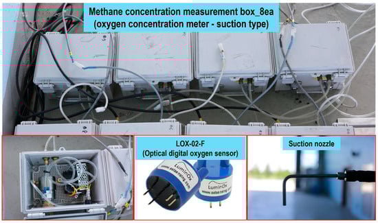
Figure 3. Gas concentration measurement sensor used in this experiment.

The sensor network used in this study consisted of two stages, as illustrated in Figure 4. In the preliminary stage, a low-resolution network with approximately 1 m spacing (eight sensors in total) was deployed to examine dispersion characteristics under representative flow-rate conditions (240 LPM and 600 LPM). However, for both conditions, only one or two sensors near the nozzle recorded noticeable concentration increases, while most sensors measured very limited variations (below 2–3%). This indicated that the spatial resolution was insufficient to capture the dispersion centerline or the concentration gradient structure.

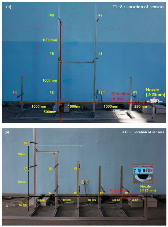
Figure 4. Sensor layouts for 1 m and 0.5 m network configurations. (a) Low-resolution sensor network with 1 m spacing. (b) High-resolution sensor network with 0.5 m spacing.

The arrows indicate the direction of methane leakage, and the dashed box highlights the nozzle with a diameter of 25 mm. All distances are given in millimeters. The labels #1–#8 denote the identification numbers of the methane sensors installed at the locations shown.Accordingly, the final experiment employed a high-resolution network consisting of eight sensors spaced at 0.5 m intervals, with several sensor positions reconfigured. This design was intended to enable detailed tracking of the dispersion pathway within the large chamber. Similar eight-channel sensor configurations have been reported in the PTAC report and continuous monitoring system (CMS) studies [21,22]. To reduce direct boundary interaction effects, the sensor array was positioned at least 0.5 m above the chamber floor and approximately 1.5 m away from the nearest wall. A detailed analysis of the high-resolution measurements and the influence of sensor-network resolution is presented in Section 4.

2.1.4. Data Acquisition and Auxiliary Equipment

As shown in Figure 5, sensor signals were collected using a data logger (GL840, Graphtec Corporation, Yokohama, Kanagawa, Japan) at a sampling frequency of 1 Hz. This sampling rate is consistent with the time resolution reported as sufficient in previous fixed-type continuous monitoring system (CMS) studies [22]. An optical gas imaging (OGI) camera (GF300, FLIR Systems, Wilsonville, OR, USA) was used as auxiliary equipment, serving only for visual confirmation of dispersion patterns rather than for quantitative analysis.

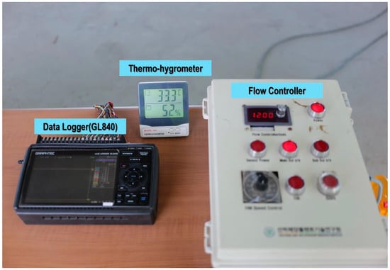
Figure 5. Instrumentation for methane release and concentration measurement.

2.1.5. Experimental Procedure

It should be noted that the methane release duration of 30 s was selected to resolve the transient dispersion behavior and sensor response characteristics during the early-stage leakage phase. Preliminary observations confirmed that the primary jet structure, plume centerline development, and LEL (5%) reach were established within this time window for all flow-rate conditions considered.

Accordingly, the selected duration is sufficient for evaluating sensor detectability, concentration gradients, and experiment–CFD agreement associated with initial leakage scenarios. Consideration of long-term accumulation under fully stagnant conditions involves different governing mechanisms and time scales and is therefore beyond the scope of the present experimental campaign.

2.2. Numerical Methodology

2.2.1. Overview of the Numerical Analysis

To compare with the experimental results, CFD simulations were performed for four flow-rate cases—240, 360, 480, and 600 LPM—using the same sensor configuration and spatial resolution as the 0.5 m high-resolution sensor network. The simulations were carried out using the commercial CFD code ANSYS Fluent (v.2023R2) [23]. The governing equations included the transient continuity equation, the Navier–Stokes equations, the energy equation, and the species-transport equation for methane–air mixtures.

This framework enabled the prediction of vertical and horizontal dispersion distances and the overall dispersion behavior under different methane flow rates.

2.2.2. Computational Domain and Mesh Configuration

The computational domain was modeled to match the experimental chamber: a fully enclosed volume of 16 m (B) × 30 m (L) × 20 m (H), with gravitational acceleration applied in the vertical direction and no background ventilation. As illustrated in Figure 6, the internal 3D geometry of the chamber was reconstructed to define the flow region.

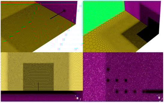
Figure 6. Mesh in computational domain.

A locally refined mesh was generated near the nozzle and the leak source to accurately resolve steep gradients, while a gradually coarsened mesh was applied further away in the far-field dispersion region. All zones were discretized using a hexcore dominant mesh, which is advantageous for representing smooth concentration fields. Refinement zones were applied around the nozzle and the sensor locations to capture localized flow variations, and the grid resolution was increased in stages to ensure stable simulation performance. Figure 6 shows the refinement regions and the resulting mesh distribution around the nozzle and sensor areas.

To minimize grid dependency—an essential requirement for CFD reliability—grid-sensitivity analyses were performed using three mesh densities. Table 3 summarizes the mesh conditions evaluated.

Table 3. Grid dependency test.

Grid Level	Cell Count (Million)	Average Relative Error E [%]	Remarks
Coarse	1.71	0.78%	Under-resolved near-nozzle region
Medium	6.45	0.62%	Grid-independent; selected for final simulations
Fine	11.30	0.58%	No significant improvement over medium grid

Simulations were conducted for meshes containing 1.70 million, 6.45 million, and 11.28 million cells, and concentration time histories were compared at the eight sensor locations for each case. Based on the evaluation of error variation with mesh refinement, the 6.45-million-cell mesh was determined to provide sufficient grid independence. All flow-rate simulations were therefore conducted using this mesh resolution.

2.2.3. Turbulence Models

Turbulent mixing and buoyancy-driven dispersion were modeled using the RNG k–ε turbulence model as the primary closure approach, as it provides improved performance for flows characterized by strong strain rates and buoyancy effects relevant to methane jet dispersion in enclosed spaces. To assess model sensitivity, additional simulations were performed using the k–ω GEKO turbulence model, which extends the SST-based k–ω formulation through internal tuning functions to enhance robustness across a wide range of flow regimes. The complete governing equations, buoyancy terms, turbulence transport equations, and model-specific coefficients for both turbulence models are provided in Appendix C and Appendix D for reproducibility [23].

2.2.4. Boundary and Initial Conditions

To reproduce methane dispersion inside a large, enclosed chamber, the numerical simulations were configured with the following boundary and initial conditions. The analysis was performed in transient mode to allow direct comparison with the time-resolved experimental measurements, and a pressure-based solver was employed. The working fluid was defined as a non-reacting ternary mixture consisting of methane (${\mathrm{C}\mathrm{H}}_4$), oxygen (${\mathrm{O}}_2$), and nitrogen (${\mathrm{N}}_2$).

The initial concentration in the chamber was set to match atmospheric composition, with 21% oxygen and 79% nitrogen, consistent with the standard assumptions used in previous indoor gas-dispersion studies [3,24]. To account for uncertainties in the diffusion characteristics of methane–air mixtures, the turbulent Schmidt number $S{c}_t$ was evaluated using three values—0.7, 0.8, and 0.9. The expanded species transport equation and diffusion closure, including the definition of the turbulent Schmidt number, are detailed in Appendix B. This range reflects commonly adopted values (0.7–1.0) reported in earlier research [10,23]. By comparing the three Schmidt-number cases, the sensitivity of the dispersion behavior and the reproducibility of the numerical model relative to the experimental data were assessed. The full boundary-condition configuration is summarized in Figure 7 and Table 4.

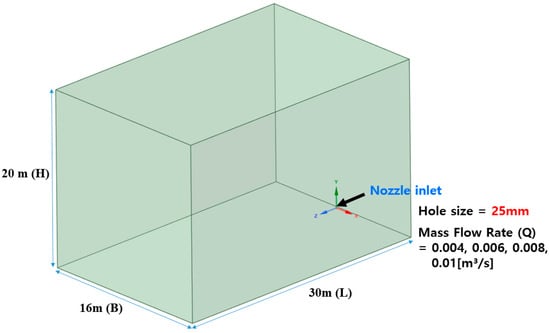
Figure 7. Computational domain and boundary conditions for CFD simulations.

Table 4. Boundary Condition.

Item	Condition
Analysis type	Transient
Solver	Pressure-based
Energy equation	On
Turbulence model	$\mathrm{RNG} k–\epsilon$$, k–\omega$ GEKO
Working fluid	$\mathrm{Methane} ({\mathrm{C}\mathrm{H}}_4$$), \mathrm{Oxygen} ({\mathrm{O}}_2$$), \mathrm{Nitrogen} ({\mathrm{N}}_2$)
Schmidt number (Sc)	0.7, 0.8, 0.9
Initial condition	Non-reacting mixture: O2 21%, N2 79%
Time step	0.01 s
Inlet	240, 360, 480, 600 LPM
Outlet	Wall (no flow)
Nozzle diameter	25 mm nozzle

The nozzle diameter was set to 25 mm, and the inlet flow rates were specified as 240, 360, 480, and 600 LPM (0.004–0.010 m³/s). Using the continuity relation $Q=vA$, the corresponding nozzle exit velocities were calculated as approximately 8.15, 12.22, 16.30, and 20.37 m/s. These velocities follow directly from the nozzle geometry and prescribed flow rates, consistent with the standard relationship between volumetric flow and jet velocity for orifices and nozzles defined in ISO 5167-2 [25]. Based on industrial vapor release modeling guidelines, methane jet velocities for small-scale leakage scenarios are commonly considered to fall within approximately 5–30 m/s [9]; thus, the 8–20 m/s inlet velocities adopted here are representative of realistic industrial leakage conditions. The mass flow rates applied at the nozzle inlet and the corresponding mass flow and exit velocities are summarized in Table 5.

Table 5. Mass Flow Rate.

Flow Rate (LPM)	Q (m3/s)	$\dot{\mathit{m}}{\mathit{C}\mathit{H}}_4$ (kg/s)	${\mathit{U}}_{\mathit{n}\mathit{o}\mathit{z}\mathit{z}\mathit{l}\mathit{e}}$ (m/s)
240	0.004	0.002605004	8.148783
360	0.006	0.003907506	12.223100
480	0.008	0.005210008	16.297466
600	0.010	0.006512511	20.371833

All chamber walls were treated as no-slip, impermeable boundaries, accounting for wall-friction effects and preventing any mass exchange through the surfaces. The outlet boundary was modeled as a closed-wall condition, reflecting the sealed nature of the experimental chamber and maintaining consistency with the laboratory setup. Gravity was applied in the vertical (y) direction at −9.81 m/s². Because methane is lighter than air, buoyancy forces significantly influence the upward dispersion behavior. To represent this effect, the Boussinesq approximation was employed, which linearizes density variations for buoyancy-driven flow. This approximation is considered valid when relative density variations remain small [23]. The full momentum equation incorporating the buoyancy closure under the Boussinesq approximation is summarized in the main text, while its complete formulation is reported in Appendix A.

The time step $\Delta t$ was set to 0.01 s, selected to satisfy the Courant–Friedrichs–Lewy (CFL) condition . Each simulation was performed for a total duration of 30 s, and after the flow field reached a quasi-steady condition, the concentration fields were time-averaged and compared with experimental measurements.

2.2.5. Numerical Procedure and Solver Settings

For the transient simulations, a time step of 0.01 s was applied, and each case was computed for a total physical time of 30 s. Pressure–velocity coupling was handled using the SIMPLE algorithm [10,23], and all transport equations were discretized using a second-order upwind scheme to ensure numerical stability and reduce truncation errors [10,23].

The simulations were executed on a 64-core parallel computing system (AMD EPYC 7543 CPU, 256 GB RAM). The average computational time was approximately 72 h per case, depending on the mesh configuration and turbulence model.

2.2.6. Sensor Points and Data Processing

Consistent with the experimental configuration, eight virtual sensor points were defined within the CFD domain. At each location, the methane volume fraction was recorded as a time-resolved signal and directly compared with the experimental measurements.

The comparison metrics included:

• Peak methane concentration at each sensor
• Concentration rise rate during the early accumulation stage
• LEL (5% vol) attainment and corresponding detection timing

These metrics reflect the sensor performance characteristics examined in the experiment and allow one-to-one validation of the numerical predictions against the high-resolution sensor network.

2.2.7. Validation Strategy

The experimental–numerical comparison was carried out using three primary indicators:

(1)

Maximum concentration capture

- Comparison of the highest methane concentration measured at each sensor.

(2)

Concentration gradient

- Evaluation of concentration differences between near-nozzle and far-field sensors, used to assess how well each model reproduces the spatial dispersion structure.

Maximum concentration levels and spatial concentration gradients have been commonly employed as qualitative and semi-quantitative indicators for assessing agreement between experiments and CFD simulations in gas-dispersion studies, particularly in evaluations of plume structure and decay behavior [3,4,5,26].

3. Experimental and Numerical Results

This section presents an analysis of the methane dispersion characteristics measured using the high-resolution sensor network with 0.5 m spacing. Prior to the main experiment, preliminary tests were conducted using a low-resolution 1 m sensor grid under two flow-rate conditions—240 LPM and 600 LPM. The preliminary results revealed that, for both conditions, only one or two sensors located near the nozzle recorded appreciable concentration levels, while most sensors measured methane concentrations below 2–3%. This indicated that the low-resolution network was insufficient for capturing the spatial structure of the dispersion centerline and concentration gradients.

Accordingly, the analysis in this chapter focuses exclusively on the high-resolution sensor network, which provided detailed concentration–time histories across the eight measurement points. Based on these data, key dispersion characteristics—including spatial dispersion patterns, detection timing, and concentration rise rates—were quantitatively evaluated and compared with the corresponding CFD predictions [9].

3.1. Experimental Results

This section presents a quantitative analysis of methane dispersion based on the concentration–time measurements obtained from the high-resolution sensor network with a 0.5 m spacing, as shown in Figure 8. The sensors were positioned within a forward range of 0.15–2.15 m and a vertical range of 0–1.0 m relative to the nozzle (Figure 5), allowing the directional characteristics of the dispersion plume and the corresponding concentration gradients to be evaluated with high spatial fidelity.

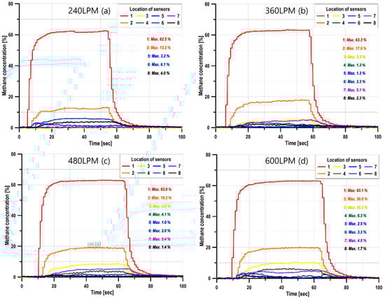
Figure 8. Time-series methane concentrations at eight sensors for four flow-rate scenarios.

3.1.1. Spatial Distribution Characteristics

Across all flow-rate conditions (240–600 LPM), the experiments consistently showed an upward-directed jet forming along the nozzle centerline, followed by lateral spreading as the plume evolved. Near the nozzle (S1), high concentrations of approximately 63% were observed regardless of flow rate. This behavior is attributed to the dominant influence of initial jet momentum and the associated turbulent structures.

As the flow rate increased, both the plume width and plume length expanded. Under the 240 LPM condition, dispersion remained primarily localized near S1 and S2 (within approximately 1 m of the nozzle). In contrast, at 480–600 LPM, the region exceeding the LEL threshold of 5% extended horizontally to approximately 2.0–2.1 m. These trends are consistently reflected in the time-resolved concentration fields presented in Figure 8a–d.

3.1.2. Detection Time Characteristics

The time at which methane was first detected at each sensor serves as a key indicator of the underlying dispersion mechanism. In all scenarios, detection occurred sequentially in the order S1 → S2 → S3 → S4, with progressively longer delays at the downstream sensors.

At the lowest flow rate (240 LPM), methane arrived at S1 after approximately 3–5 s, at S2 after 6–8 s, and at S3 after 10–15 s, with even longer delays at the far-field sensors (S5–S8). At 600 LPM, the increase in jet momentum led to substantially faster dispersion: methane was detected at S1 within 1–3 s, at S2 within 3–5 s, and at S3 within 5–9 s—representing a reduction of more than 40% relative to the low-flow case.

Thus, as illustrated in Figure 8a–d, detection time decreases nonlinearly with increasing flow rate, and the spatial region influenced by the plume expands accordingly.

3.1.3. Initial Concentration Increase Rates

The early-stage concentration increases rates (ΔC/Δt) over the first 10–20 s was compared for all sensors. A systematic decay in slope was observed as the distance from the nozzle increased:

(1)

S1: 6–8%/s (jet core region, momentum-dominated)

(2)

S2: 3–5%/s (transition region)

(3)

S3: 1–3%/s (mixed buoyancy–turbulence region)

(4)

S4–S8: 0.1–0.5%/s (dilution-dominated region)

Overall, the concentration increases rates grew with flow rate, reflecting intensified turbulence levels in the jet core. Notably, S2 and S3 exhibited the strongest sensitivity to flow rate, as these sensors lie within the transitional region where momentum-dominated behavior shifts toward buoyancy-dominated dispersion, as also indicated in Figure 8a–d.

3.1.4. Integrated Comparison of the Four Scenarios

Figure 8 compares the experimentally observed and CFD-predicted methane dispersion patterns for the different flow-rate conditions. For intermediate and high flow rates, the simulations closely reproduced the spatial extent and overall structure of the measured plumes, while larger discrepancies were observed in the low-flow case, particularly in the far-field region. These comparisons confirm that the agreement between experiments and simulations improves with increasing release rate.

3.2. Numerical Simulation Results

This section presents the CFD results obtained under the operating conditions described in Section 2. The simulations were conducted for the same flow rates as the experiments (240–600 LPM), and the spatial dispersion characteristics and time-resolved concentration histories at the sensor locations were compared to evaluate the reproducibility of the numerical model. First, iso-surface visualizations were used to examine the spatiotemporal features of the methane plume (Section 3.2.1). This is followed by sensor-based quantitative comparisons of maximum concentration, detection timing, and dispersion distance (Section 3.2.2, Section 3.2.3 and Section 3.2.4). Figure 9 presents OGI visualizations of the methane plume at t = 12 s for four representative leak rates (240–600 LPM).

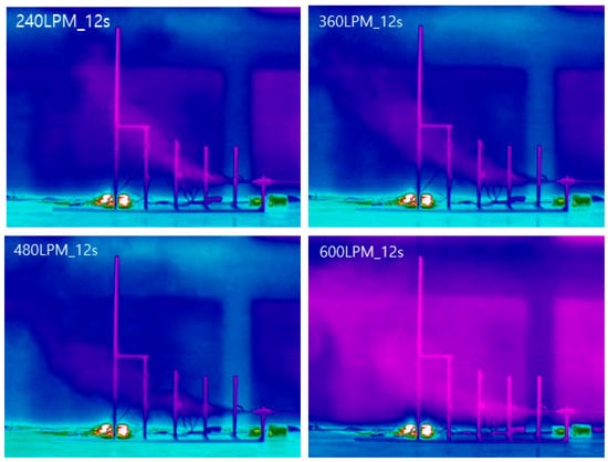
Figure 9. OGI visualization of methane plume for four leak rates at t = 12 s. (a) 240 LPM, (b) 360 LPM, (c) 480 LPM, (d) 600 LPM. The color variations represent temperature-dependent infrared intensity and are used for qualitative visualization only.

3.2.1. CFD-Based Spatial Dispersion Structure

As illustrated in Figure 10a–d, the iso-surface visualizations show that, for all flow rates, a strong upward-directed jet forms during the initial 3–6 s, after which turbulent diffusion progressively widens the plume. At 240 LPM, the dispersion centerline remains relatively narrow, whereas at 600 LPM the increased jet momentum produces a wider and more rapidly expanding plume.

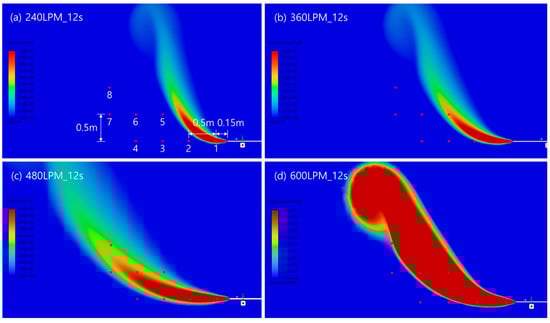
Figure 10. CFD-predicted Methane concentration fields (volume fraction) with overlaid sensor positions at t = 12 s (a) 240 LPM, (b) 360 LPM, (c) 480 LPM, (d) 600 LPM).

The 5% volume-fraction iso-surface at t = 12 s extends horizontally to approximately 1.0 m at 240 LPM, 2.0 m at 480 LPM, and 2.1 m at 600 LPM. This trend closely matches the experimental observations, indicating that the CFD model successfully captures the dependence of plume width on the inlet flow rate.

3.2.2. Comparison of Maximum Concentrations

As shown in Figure 11a–d, the CFD results closely reproduced the sensor-specific maximum concentrations observed in the experiments. For instance, under the 480 LPM condition, the maximum concentrations at sensors S1–S4 differed from the experimental values by only −0.6% to +0.4%. Even in the low-concentration regions (S5–S8), discrepancies generally remained within ±1–2%.

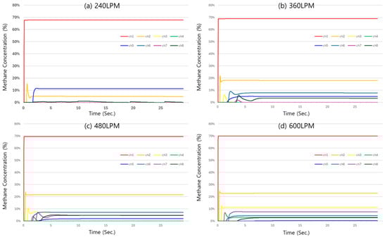
Figure 11. CFD-predicted Methane concentration time histories at eight sensor locations for four leak rates (a) 240 LPM, (b) 360 LPM, (c) 480 LPM, (d) 600 LPM.

These results demonstrate that the adopted turbulence models (RNG $k–\epsilon$ and $k–\omega$ GEKO) can reliably represent the balance between jet momentum, buoyancy effects, and turbulent mixing, thereby reproducing the dispersion behavior in a large enclosed space with high fidelity.

3.2.3. Reproducibility of Detection Timing and Concentration Gradients

The CFD simulations also reproduced the characteristic increase in detection delay from S1 → S2 → S3 → S4, consistent with the experimental findings. Differences in detection time between simulation and experiment were generally within ±1–2 s, indicating strong agreement. The concentration rise rates likewise followed the same spatial ordering as in the measurements, confirming that the numerical model accurately reflects the changes in dispersion speed and local mixing rates.

3.2.4. Temporal Evolution of Methane Concentration

Under the 600 LPM condition, the numerical results showed methane concentrations in close agreement with the experimental measurements. The maximum concentrations at sensors S1–S4 were 62.9%, 19.4%, 10.0%, and 6.0%, respectively, compared with experimental values of 63.1%, 20.0%, 10.3%, and 6.3%, with discrepancies within 1–3%. The high-concentration region developed upward along the nozzle centerline, while the low-concentration region (2–5%) spread toward the mid–upper portions of the chamber, and the plume eventually decelerated and accumulated near the walls, consistent with experimental observations.

Figure 11 presents the CFD-predicted concentration time histories at the eight sensor locations for all flow-rate conditions. In all cases, the simulations capture the rapid concentration increase near the leak source (S1–S2), followed by progressively delayed and attenuated responses at downstream sensors due to jet momentum decay, buoyancy-driven rise, and turbulent mixing. As the flow rate increases from 240 to 600 LPM, both the concentration rise rate and the time to reach quasi-steady behavior decrease, with signals at S1–S4 stabilizing within approximately 10–15 s at intermediate and high flow rates. In contrast, under the low-flow condition, downstream sensors exhibit slower and weaker responses, reflecting increased sensitivity to buoyancy effects in the dilute far-field region.

3.2.5. Quantitative Comparison Between Experiments and Simulations

Table 6 summarizes the comparison between experimentally measured and CFD-predicted maximum methane concentrations at each sensor location for the four leakage conditions. For all flow rates, strong agreement was observed in the high- and mid-concentration regions (S1–S4), with relative differences generally within ±3%. These sensors are located within or near the jet core region, where dispersion is dominated by initial jet momentum and turbulent mixing.

Table 6. Experimental vs. CFD Maximum Concentration Comparison.

Flow Rate (LPM)	Case	S1	S2	S3	S4	S5	S6	S7	S8
240	Experiment	62.5	13.2	0.0	0.0	3.2	6.1	0.0	4.0
	CFD	67.9	15.4	0.0	0.0	11.7	0.0	0.0	1.1
	Error (%)	+8.0	+14.3	0.0	0.0	+72.6	−100.0	0.0	−72.5
360	Experiment	63.3	17.9	5.2	1.3	1.3	3.3	5.1	2.3
	CFD	68.9	21.7	6.1	0.0	4.9	9.0	1.9	5.9
	Error (%)	+8.1	+17.5	+14.8	0.0	+73.5	+63.3	−62.7	+61.0
480	Experiment	63.0	19.2	8.8	4.1	1.0	2.0	5.4	1.4
	CFD	69.6	23.9	10.7	3.7	2.0	7.2	7.1	5.0
	Error (%)	+9.5	+19.7	+17.8	−10.8	+50.0	+72.2	+23.9	+72.0
600	Experiment	63.1	20.0	10.3	6.3	2.3	3.3	4.8	1.7
	CFD	70.0	25.0	12.6	6.9	3.0	4.4	7.7	2.7
	Error (%)	+9.9	+20.0	+18.3	+8.7	+30.0	+25.0	+37.7	+37.0

Note: Large relative errors occur in dilute far-field regions where experimental concentrations are close to zero; these values reflect sensitivity to plume centerline position rather than absolute prediction failure.

Larger relative differences were observed at downstream sensor locations in the low-concentration far-field region (S5–S7), particularly under the low-flow condition of 240 LPM. In this case, the CFD simulations predicted near-zero concentrations at certain lateral sensor locations, whereas measurable methane concentrations were detected experimentally. This discrepancy corresponds to a positional offset between the predicted and measured plume trajectories, resulting in reduced overlap between the plume centerline and specific sensor locations.

Despite these localized differences, the CFD simulations reproduced the overall dispersion patterns, temporal evolution of methane concentration, and LEL (5%) reach across all flow-rate conditions. Interpretation of the underlying mechanisms and implications of these discrepancies is addressed in the Discussion section.

4. Analysis and Discussion

This section provides an integrated interpretation of the experimental and numerical findings presented in Section 3. The major dispersion characteristics of methane leakage are analyzed with respect to flow rate, turbulence-model selection, grid resolution, and sensor-network spacing. Furthermore, the practical applicability and limitations of the CFD model developed in this study are discussed to identify opportunities for future improvement.

4.1. Overview of Experimental–CFD Agreement

To support the primary objective of this study—namely, quantifying the influence of sensor-network resolution on methane dispersion measurement—the experimental results are first interpreted in conjunction with CFD predictions. Comparisons between the experimental measurements and CFD predictions reveal a clear dependence of agreement on the leakage flow rate. For the intermediate and high flow-rate cases (360–600 LPM), key dispersion characteristics—including maximum concentration in the high-concentration core (S1–S3), spatial concentration gradients, detection timing, and overall dispersion distance—were reproduced with strong fidelity. In these cases, the predicted dispersion distance differed from the measurements by approximately ±0.1 m, indicating robust predictive performance.

In contrast, the low-flow condition (240 LPM) exhibited noticeably larger discrepancies in the low-concentration far-field region (S5–S7). While the overall dispersion pattern and temporal evolution were captured, differences in plume trajectory led to reduced agreement at certain downstream sensor locations. These flow-rate-dependent trends are consistently observed across the experimental and numerical datasets and form the basis for the detailed interpretation presented in the following sections.

4.2. Impact of Turbulence Model and Grid Resolution on Predictive Accuracy

The turbulence models adopted in this study—RNG $k–\epsilon$ and $k–\omega$ GEKO—have been applied to jet and buoyancy-driven turbulent flows and generally performed well [18]. Nevertheless, the centerline shift observed under low-flow conditions can be explained by several factors related to model formulation and mesh resolution:

(1)

Reproduction of initial jet momentum

In the experiment, internal turbulence generated within the piping system and nozzle roughness affects the initial jet profile. In contrast, CFD simulations typically assume an idealized velocity profile, which may cause deviations in the early jet energy level [27].

(2)

Mesh resolution near the nozzle

Insufficient grid refinement around the nozzle reduces accuracy in predicting jet spreading rates and turbulence generation. This can be particularly pronounced under low-flow conditions, where jet decay rate and buoyancy transition are highly sensitive to mesh quality [26,28].

(3)

Treatment of buoyancy-production terms in turbulence models

RNG $k–\epsilon$ and GEKO incorporate buoyancy-density effects through correction factors, but these adjustments may not fully capture the rapid momentum-to-buoyancy transition at low flow rates [18]. As a result, the actual transition point may not be reproduced precisely.

These factors contribute to greater relative errors in the low-concentration region. However, such limitations can be mitigated through finer mesh refinement, dependence on hybrid RANS–LES or full LES models, or improved representation of inlet turbulence characteristics [4].

For the low-flow-rate condition, the discrepancies observed between experiments and simulations—particularly the forward shift of the plume centerline and the larger relative errors at far-field sensor locations—were primarily attributed to an earlier transition from momentum-dominated to buoyancy-dominated dispersion in the CFD results.

However, it should be noted that additional physical mechanisms not explicitly modeled in the present study may also contribute to these deviations. These include wall boundary-layer development, surface roughness effects, and weak thermal stratification arising from residual heat transfer between the chamber walls and the surrounding environment [24,29]. Although methane adsorption on typical chamber wall materials is generally negligible over the short experimental time scales considered here, such effects cannot be entirely excluded in dilute, low-velocity regions.

In this study, smooth and adiabatic wall boundary conditions were adopted to isolate the dominant dispersion mechanisms and to maintain consistency between the experimental and numerical frameworks across all cases. This modeling choice is consistent with common practice in large-scale enclosed gas-dispersion studies and facilitates relative comparison of dispersion trends across different flow rates. Nevertheless, under low-flow conditions where buoyancy effects become increasingly sensitive to secondary influences, the simplified wall treatment may limit predictive accuracy in the far-field region [24,29]. These limitations are acknowledged here and represent an important direction for future work involving more detailed wall characterization and coupled heat-transfer modeling.

4.3. Influence of Sensor-Network Resolution on Measurement Accuracy and Model Validation

The preliminary experiments employed a low-resolution, 1 m–spaced sensor network under 240 LPM and 600 LPM conditions. In both cases, significant under-resolution of the plume width resulted in only the near-nozzle sensors (S1–S2) detecting meaningful concentrations, while most other sensors recorded less than 2–3%. This outcome aligns with prior studies showing that coarse sensor spacing cannot reliably capture the structure of the dispersion centerline or the dilute plume region [22].

Because this under-resolution caused critical plume features—such as centerline position, concentration gradients, and the momentum-to-buoyancy transition zone—to be inadequately resolved, the final experiments were conducted using a 0.5 m high-resolution network with adjusted sensor placement.

With the high-resolution network, the plume centerline could be continuously tracked from S1 to S4, and the spatial variations in concentration rise rate became clearly distinguishable. In particular, the mid-concentration region (approximately 2–5%) was resolved sufficiently to enable accurate validation against CFD predictions. These findings demonstrate that high-resolution sensing substantially improves the accuracy of CFD validation for confined-space methane dispersion, consistent with the results reported in earlier work [7].

4.4. Interpretation of Flow-Rate-Dependent Dispersion Behavior

The flow-rate-dependent trends summarized in Section 4.1 can be interpreted in terms of the relative contributions of jet momentum and buoyancy during plume development. As the leakage flow rate increases, the initial jet momentum flux becomes sufficiently large to stabilize turbulent mixing and to suppress the early influence of buoyancy, resulting in improved agreement between experimental observations and CFD predictions [30]. For the intermediate and high flow-rate cases (360–600 LPM), this momentum-dominated regime enables accurate reproduction of plume structure, concentration gradients, detection timing, and overall dispersion extent.

In contrast, under the low-flow condition (240 LPM), the reduced jet momentum causes the plume to become sensitive to buoyancy effects at an earlier stage of development. This earlier transition from momentum-dominated to buoyancy-dominated dispersion can promote an earlier shift of the plume centerline, as accelerated jet decay and centerline development have been reported to be sensitive to inlet turbulence characteristics 27]. Experimentally, the plume centerline transition was observed around the S6 region (approximately 1.0–1.2 m downstream), whereas the CFD simulations predicted an earlier transition near the S5 region (approximately 0.5–0.75 m). This difference indicates a slightly faster jet decay in the numerical model, leading to an earlier onset of buoyancy-driven ascent and consequently lower predicted concentrations at lateral far-field sensor locations [31].

From a practical perspective, this behavior implies that CFD predictions under low-flow, buoyancy-sensitive conditions should be interpreted with caution in the dilute far-field region. In such cases, RANS-based simulations may provide a conservative lower bound for methane concentrations at downstream lateral locations, as has been reported in previous studies on buoyant jet dispersion in enclosed or weakly ventilated environments [18,31,32]. Accordingly, when CFD results are applied to sensor placement or safety assessment, additional spatial margins beyond the CFD-predicted plume boundary are recommended for low-momentum leakage scenarios.

Overall, the observed trend—improved experiment–CFD agreement at higher flow rates and increased sensitivity to buoyancy effects at lower flow rates—is consistent with the established characteristics of buoyant jet dispersion in enclosed spaces [18,33,34]. These flow-rate-dependent characteristics directly influence the spatial resolution required for reliable gas detection, motivating the sensor placement considerations discussed in the following section.

4.5. Implications for Sensor Placement and Practical Application

Based on the experimentally validated dispersion characteristics, the present study provides insight into the applicability of CFD-based predictions for sensor placement in large enclosed spaces. The results indicate that predictive reliability varies across concentration regimes, underscoring the need to align sensor-network resolution with dominant dispersion features.

In the high- and mid-concentration regions near the leak source and the LEL threshold (S1–S4), excellent agreement between experiments and simulations was achieved for all flow conditions. These regions are governed primarily by jet momentum and turbulent mixing, enabling reliable CFD-based assessment of hazardous gas accumulation and LEL reach.

In contrast, dispersion in the low-concentration far-field region is strongly influenced by buoyancy–turbulence interactions. Under low-flow conditions, CFD predictions tended to underpredict methane concentrations due to sensitivity in plume trajectory. Accordingly, application of CFD results in this region should incorporate conservative spatial margins, particularly when used to inform sensor placement for early warning or accumulation monitoring.

With respect to sensor-network resolution, the present findings suggest that a spacing of approximately 1.0 m is sufficient for characterizing high-concentration regions, whereas a refined spacing of 0.5 m or less is required to reliably resolve mid- and low-concentration regions. These recommendations are derived from uniform sensor layouts adopted to isolate the effect of spatial resolution and to ensure direct experiment–CFD comparability.

It is emphasized that the uniform sensor configurations employed here are not intended to represent optimal deployment strategies for real shipboard compartments, which are characterized by structural complexity and ventilation-induced preferential flow paths. Rather, the experimentally validated dispersion trends provide physically grounded lower-bound requirements for sensor spacing, serving as a reference framework for subsequent risk-based or optimization-oriented sensor placement studies. The applicability of these implications should therefore be interpreted within the experimental scope and limitations described in the following section.

4.6. Limitations and Interpretation Range

The results of this study should be interpreted within the context of the experimental conditions employed. The experiments were conducted in a large, unobstructed, and non-ventilated chamber, with sensor locations positioned away from direct wall and floor interaction. This configuration was deliberately selected to minimize boundary-induced disturbances and to isolate the dominant dispersion mechanisms—jet momentum, buoyancy-driven rise, and turbulent mixing—under controlled baseline conditions.

Under these conditions, the experimentally validated CFD model provides reliable insight into early-stage dispersion behavior and sensor response characteristics following the onset of methane leakage. In particular, the present results are well suited for examining plume formation, centerline development, concentration gradients, and LEL (5%) reach during the transient leakage phase. However, the findings are not intended to directly represent scenarios dominated by long-term accumulation, strong ventilation flows, or complex structural interactions typically encountered in realistic shipboard compartments.

In such scenarios, additional physical effects—including ventilation-induced advection, wall roughness, equipment-induced flow obstruction, and heat-transfer-driven stratification—may significantly alter dispersion behavior and concentration evolution over longer time scales. These effects were intentionally excluded from the present study to preserve experimental–numerical comparability and to enable systematic evaluation of sensor-network resolution under well-defined conditions.

Accordingly, the present study establishes a reference framework rather than a comprehensive representation of all shipboard leakage scenarios. The experimentally validated dispersion trends reported here are intended to serve as a baseline against which more complex configurations—such as obstructed geometries, non-uniform sensor deployment, and ventilated compartments—can be systematically evaluated in future experimental or numerical investigations.

5. Conclusions

This study quantitatively characterized methane dispersion behavior in a large enclosed space (30 × 16 × 20 m) and validated the predictive capability of a CFD model using high-resolution sensor-network measurements. Preliminary experiments using a 1 m sensor spacing revealed that, under both representative flow-rate conditions (240 and 600 LPM), only the sensors located near the nozzle detected meaningful concentration changes, indicating insufficient spatial resolution for identifying the dispersion centerline and concentration gradients. Consequently, a high-resolution 0.5 m sensor network was deployed, enabling accurate capture of key dispersion features, including the plume centerline, concentration gradients, and detection timing.

The high-resolution measurements revealed that an upward-directed jet formed at the early stage for all flow rates, with the plume width and the extent of the low-concentration region (approximately 2–5%) increasing nonlinearly with flow rate. Detection times were shortened as the flow rate increased, reflecting the strengthening influence of momentum-driven dispersion. The spatial dependence of early concentration rise rates was also clearly distinguished across sensor locations. These measurements provided the spatial and temporal fidelity necessary to resolve large-scale indoor methane dispersion mechanisms.

CFD simulations were performed using the RNG $k–\epsilon$ and $k–\omega$ GEKO turbulence models under identical boundary and domain configurations as the experiments. The CFD model reproduced the time-resolved concentration histories, maximum concentration values, and concentration rise rates with high accuracy. In the high- and mid-concentration regions, the discrepancies remained within ±3%, and even in the low-concentration region the overall dispersion trends were captured reliably. However, for low-flow conditions, increased sensitivities associated with early jet decay and the momentum-to-buoyancy transition resulted in larger deviations at select sensor locations.

Overall, this work quantitatively clarifies methane dispersion behavior in a large enclosed environment using high-resolution experimental data and demonstrates that the CFD model achieves sufficient accuracy for practical prediction of real-world dispersion phenomena. The findings provide a robust foundation for establishing gas-detector placement strategies and safety-design criteria in LNG-fueled vessels, fuel-gas supply modules, engine rooms, and other industrial or marine compartments. Future research should extend the experiments to diverse compartment geometries, piping arrangements, and ventilation conditions, and incorporate LES-based turbulence modeling and adaptive mesh refinement (AMR) to further improve predictive accuracy, particularly in low-concentration regions.

References

- Cho, Y.; Ulrich, B.A.; Zimmerle, D.J.; Smits, K.M. Estimating natural gas emissions from underground pipelines using surface concentration measurements. Environ. Pollut. 2020, 267, 115514. [Google Scholar] [CrossRef]
- Rew, P.J.; Spencer, H. A framework for ignition probability of flammable gas clouds. In Institution of Chemical Engineers Symposium Series; Hemsphere Publishing Corporation: Washington, DC, USA, 2007. [Google Scholar]
- Li, L.; Choi, J.; Bang, J.; Lee, S.; Kim, D. Numerical investigation of LNG gas dispersion in a confined space: An engineering model. J. Mech. Sci. Technol. 2017, 31, 4533–4540. [Google Scholar] [CrossRef]
- Tominaga, Y.; Stathopoulos, T. CFD simulation of near-field pollutant dispersion in the urban environment: A review of current modeling techniques. Atmos. Environ. 2013, 79, 716–730. [Google Scholar] [CrossRef]
- Liu, A.; Xu, C.; Lu, X.; Zhou, X.; Xu, W. Coupling effect of multiple factors on diffusion behavior of leaking natural gas in utility tunnels: A numerical study and PIV experimental validation. J. Nat. Gas Sci. Eng. 2023, 118, 205086. [Google Scholar] [CrossRef]
- National Physical Laboratory (NPL). ENV52: Framework for Classifying Methane Monitoring Requirements, Emission Sources and Monitoring Methods; NPL Report CSSC 0001; National Physical Laboratory: Teddington, UK, 2024. [CrossRef]
- Sun, L.; Chen, X.; Zhang, B.; Mu, C.; Zhou, C. Optimization of gas detector placement considering scenario probability and detector reliability in oil refinery installation. J. Loss Prev. Process Ind. 2020, 66, 104131. [Google Scholar] [CrossRef]
- Newman, T.; Nemeth, C.; Jones, M.; Jonathan, P. Deep Learning Surrogates for Real-Time Gas Emission Inversion. arXiv 2025, arXiv:2506.14597. [Google Scholar] [CrossRef]
- Center for Chemical Process Safety. Guidelines for Use of Vapor Cloud Dispersion Models, 2nd ed.; John Wiley & Sons: Hoboken, NJ, USA, 2010. [Google Scholar]
- Ferziger, J.H.; Perić, M.; Street, R.L. Computational Methods for Fluid Dynamics, 4th ed.; Springer: Berlin/Heidelberg, Germany, 2020. [Google Scholar]
- Quarteroni, A.; Veneziani, A.; Vergara, C. Geometric multiscale modeling of the cardiovascular system, between theory and practice. Comput. Methods Appl. Mech. Eng. 2016, 302, 193–252. [Google Scholar] [CrossRef]
- Calabrese, M.; Portarapillo, M.; Di Nardo, A.; Venezia, V.; Turco, M.; Luciani, G.; Di Benedetto, A. Hydrogen Safety Challenges: A Comprehensive Review on Production, Storage, Transport, Utilization, and CFD-Based Consequence and Risk Assessment. Energies 2024, 17, 1350. [Google Scholar] [CrossRef]
- Amirjani, A.; Yousefi, M.; Cheshmaroo, M. Parametrical Optimization of Stent Design: A Numerical-Based Approach. Comput. Mater. Sci. 2014, 88, 102–110. [Google Scholar] [CrossRef]
- Zimmerle, D.J.; Williams, L.L.; Vaughn, T.L.; Quinn, C.; Subramanian, R.; Duggan, G.P.; Willson, B.; Opsomer, J.D.; Marchese, A.J.; Martinez, D.M.; et al. Methane Emissions from the Natural Gas Transmission and Storage System in the United States. Environ. Sci. Technol. 2015, 49, 9374–9383. [Google Scholar] [CrossRef]
- Ravikumar, A.P.; Sreedhara, S.; Wang, J.; Englander, J.; Roda-Stuart, D.; Bell, C.; Zimmerle, D.; Savarese, S. Single-blind inter-comparison of methane detection technologies—Results from the Stanford/Environmental Defense Fund (EDF) Mobile Monitoring Challenge. Elem. Sci. Anth 2019, 7, 37. [Google Scholar] [CrossRef]
- Crystals Editorial Board. Materials and Methods section examples—Use of CP-grade methane gas (≥0.995 purity) in hydrate experiments. Crystals 2021, 11, 1256. [Google Scholar]
- ISO 6145-7:2018; Gas Analysis—Preparation of Calibration Gas Mixtures—Part 7: Thermal Mass-Flow Controllers. International Organization for Standardization: Geneva, Switzerland, 2018.
- Taherian, M.; Mohammadian, A. Buoyant Jets in Cross-Flows: Review, Developments, and Applications. J. Mar. Sci. Eng. 2021, 9, 61. [Google Scholar] [CrossRef]
- NFPA 69; Standard on Explosion Prevention Systems. National Fire Protection Association: Quincy, MA, USA, 2019.
- IEC 60079-29-2; Explosive Atmospheres—Part 29-2: Gas Detectors—Selection, Installation, Use and Maintenance of Detectors for Flammable Gases and Oxygen. International Electrotechnical Commission: Geneva, Switzerland, 2015.
- PTAC (Petroleum Technology Alliance Canada). Evaluation of Methane Detection Technologies—Final Report; PTAC Technical Report: Calgary, Canada, 2018. Available online: https://www.ptac.org (accessed on 6 September 2025).
- Daniels, W.S.; Jia, M. Detection, localization, and quantification of single-source methane emissions on oil and gas production sites using point-in-space continuous monitoring systems. Elem. Sci. Anthr. 2024, 12, 00110. [Google Scholar] [CrossRef]
- ANSYS Inc. ANSYS Fluent Theory Guide, Release 2023 R1; ANSYS Inc.: Canonsburg, PA, USA, 2023. [Google Scholar]
- Britter, R.E.; Hanna, S.R. Flow and dispersion in urban areas. Annu. Rev. Fluid Mech. 2003, 35, 469–496. [Google Scholar] [CrossRef]
- ISO 5167-2; Measurement of Fluid Flow by Means of Pressure Differential Devices Inserted in Circular Cross-Section Conduits—Part 2: Orifice Plates. International Organization for Standardization: Geneva, Switzerland, 2003.
- CH-15-002; Effect of CFD Grid Resolution and Turbulent Quantities on the Jet-Flow Prediction. ASHRAE: Peachtree Corners, GA, USA, 2015.
- Virani, N.; Roussinova, V.; Balachandar, R. Influence of nozzle inlet initial turbulence level on the development of an axisym-metric turbulent jet. In Proceedings of the 29th Annual Conference of the Computational Fluid Dynamics Society of Canada, Windsor, ON, Canada, 27–29 July 2021. [Google Scholar]
- Hassanzadeh, H.; Eslami, A.; Taghavi, S.M. Positively buoyant jets: Semiturbulent to fully turbulent regimes. Phys. Rev. Fluids 2021, 6, 054501. [Google Scholar] [CrossRef]
- Papanikolaou, E.; Venetsanos, A.G.; Bartzis, J.G. The ADREA-HF CFD code for consequence assessment of hydrogen applications. Int. J. Hydrogen Energy 2010, 35, 3908–3918. [Google Scholar] [CrossRef]
- Mirajkar, H.N.; Mukherjee, P.; Balasubramanian, S. On the dynamics of buoyant jets in a linearly stratified ambient. Phys. Fluids 2023, 35, 016609. [Google Scholar] [CrossRef]
- He, Z.; Zhang, H.; Zhang, H.; Ukpong Okon, S.; Zhu, R. Particle dynamics in horizontal buoyant jets within linearly stratified environments. Environ. Fluid Mech. 2025, 25, 22. [Google Scholar] [CrossRef]
- Pope, S.B. Turbulent Flows; Cambridge University Press: Cambridge, UK, 2000. [Google Scholar]
- García-Alba, J.; Bárcena, J.F.; García, A. Zonation of positively buoyant jets interacting with the water-free surface quantified by physical and numerical modelling. Water 2020, 12, 1324. [Google Scholar] [CrossRef]
- Cao, Y.; Ooi, A.; Philip, J. Characteristics of planar buoyant jets and plumes in a turbulent channel crossflow from direct nu-merical simulations. Environ. Fluid Mech. 2024, 24, 1047–1074. [Google Scholar] [CrossRef]
Disclaimer/Publisher’s Note: The statements, opinions and data contained in all publications are solely those of the individual author(s) and contributor(s) and not of MDPI and/or the editor(s). MDPI and/or the editor(s) disclaim responsibility for any injury to people or property resulting from any ideas, methods, instructions or products referred to in the content. |
© 2026 by the authors. Licensee MDPI, Basel, Switzerland. This article is an open access article distributed under the terms and conditions of the Creative Commons Attribution (CC BY) license.