Abstract
In the context of building a new type of power system, the optimal operation of high-proportion new-energy distribution networks (HNEDNs) is a current hot topic. In this paper, a stochastic distribution robust optimization method for HNEDNs that considers energy-storage refinement modeling is proposed. First, an energy-storage lifetime loss model based on the rainfall-counting method is constructed, and then an optimal operation model of an HNEDN considering energy storage refinement modeling is constructed, aiming to minimize the total operation cost while taking into account the energy cost and the penalty cost of abandoning wind and solar power. Then, a source-load uncertainty model of HNEDN is constructed based on the Wasserstein distance and conditional value at risk (CvaR) theory, and the HNEDN optimization model is reconstructed based on the stochastic distribution robust optimization method; based on this, the multiple linearization technique is introduced to approximate the reconstructed model, which aims to both reduce the difficulty in solving the model and ensure the quality of the solution. Finally, the modified IEEE 33-bus power distribution system is used as an example for case analysis, and the simulation results show that the method presented in this paper, through reducing the loss of life in the battery storage device, can reduce the average daily energy storage depreciation cost compared to an HNEDN optimization method that does not take the energy storage life loss into account; this, in turn, reduces the total operating cost of the system. In addition, the stochastic distribution robust optimization method used in this paper can adaptively adjust the economy and robustness of the HNEDN operation strategy according to the confidence level and the available historical sample data on new energy-output prediction errors to obtain the optimal HNEDN operation strategy when compared with other uncertainty treatment methods.
1. Introduction
In the context of dual carbon goals and power system transformation, renewable energy sources like wind and solar photovoltaics are being integrated into distribution networks at an unprecedented rate. However, the intermittency and stochasticity introduced by their high-penetration integration pose new challenges to the secure, economical, and flexible dispatching of distribution networks. A High-proportion New-Energy Distribution Network (HNEDN) refers to distribution networks featuring the large-scale integration of new-energy generation, flexible loads, and energy storage resources. Operators must perform rational energy scheduling to meet the user-side load demand while minimizing operating costs and maximizing renewable energy utilization rates. Therefore, investigating optimal operational strategies for HNEDNs holds significant theoretical significance and engineering value.
Numerous studies have presented optimal operation methods for HNEDNs. For example, Reference [1] proposes an optimal dispatch methodology that considers the power quality issues posed by energy storage systems and their distributed generation. Reference [2] ignores renewable energy and load uncertainty. Reference [3] proposes a multi-stage planning strategy that considers operational reliability. It clear that one of the key issues that needs to be solved in the operation of HNEDNs is how to cope with the uncertainties in a high proportion of new-energy sources. These uncertainties can lead to the formulation of HNEDN day-ahead operation strategies that struggle to adapt to the fluctuations and stochastic changes in the new-energy output, which affects the operating economy and stability of the HNEDN. Although Reference [4] has limitations in its scenario generation and uncertainty modeling approach, uncertainty treatment is considered. Stochastic programming (SP) and robust optimization (RO) are two common methods for handling uncertainty in HNEDNs. Reference [5] uses a stochastic optimization method to deal with the uncertainty problem in distributed photovoltaic (PV) output. Reference [6] applies a multi-stage stochastic planning method for distributed generator (DG) uncertainty. However, the latter suffers from data-dependency and a poor real-time performance. Reference [7] proposes a three-level robust optimization model combined with the Benders decomposition algorithm to deal with the uncertainty caused by fluctuations in PV generation and load demand. Reference [8] combines hybrid stochastic planning and robust optimization methods, taking into account the advantages of both through considering the probability distribution characteristics of uncertain parameters, while avoiding conservatism and reducing computational complexity. SP relies on a large number of historical samples and provides a good portrayal of typical output scenarios, but is usually overly optimistic and prone to ignoring extreme cases; RO guarantees feasibility in the worst operating scenarios, but may lead to escalating operating costs due to its over-conservatism. In recent years, distributed robust optimization (DRO) has received much attention as a compromise solution, achieving a balance between operational risk and cost by constructing data-driven uncertainty sets, as well as having a better adaptive adjustment capability when compared to stochastic planning and robust optimization methods. Reference [9] proposes an adaptive robust optimization model embedded in a multi-timescale problem of long-term planning, day-ahead scheduling, and intra-day adjustments. It introduces a local uncertainty management strategy to proactively manage the uncertainty of renewable energy and load demand. Reference [10] proposes a two-tier robust planning model based on adjustable, typical budget sets for seasonal fluctuations in renewable energy, which optimizes robustness across seasons through proactive management elements, but its scenario-generalization capability is limited. However, most of the existing DRO studies focus only on a single new-energy output or treat load and new-energy uncertainty uniformly, ignoring the differences between the two in terms of their distribution characteristics and prediction accuracy, making it difficult to apply the HNEDN operation strategy in practice. In fact, the source-load uncertainty has different characteristics: the probability distribution of new-energy output uncertainty is difficult to determine, and the prediction accuracy decreases rapidly over time, which makes prediction difficult, while the probability distribution of load prediction is usually considered to obey the normal distribution and the prediction accuracy is higher. In addition, the HNEDN optimization operation model, constructed based on the robust distribution optimization method, is usually more complex and has strong non-convexity, which makes it difficult to efficiently determine the global optimal solution.
On the other hand, the use of flexibility resources such as energy storage systems (ESS) and demand response (DR) in HNEDNs also provide a rich means of regulation for the optimal operation of HNEDNs. Reference [11] proposes a multi-timescale scheduling method for distribution networks that takes into account demand response and comprehensive user satisfaction, which ensures the interests of users while effectively improving the operation of distribution networks. Reference [12] constructs an economic mixed-integer linear programming model, taking into account the demand-response action time and storage charge/discharge timing constraints to realize a smart distribution network with multi-temporal coordinated scheduling. Reference [13] proposes a joint planning approach combining battery ESS and demand-side response (DSR), which aims to smooth wind power fluctuations, reduce network losses, and improve economics. Reference [14] puts forward a two-layer stochastic optimization model for the cooperation of transmission and distribution networks, which suppresses the fluctuations in renewable energy through the joint scheduling of energy storage systems and demand response. Reference [15] designs an energy storage allocation model based on the flexible insufficiency rate index of the power market to quantify the impact of different operation strategies on the regulation capabilities of the distribution network. Reference [7] establishes a source-network–load-storage cooperative optimal dispatch model to improve the economy and stability of the distribution network in terms of siting and capacity determination, uncertainty modeling, and multi-objective optimization. The literature discussed above provides a significant reference for the optimized operation of HNEDNs. However, the majority of the existing literature focuses only on modeling the constraint relationships between the state of charge (SOC) and the charge/discharge power of ESS, ignoring the impact of the cyclic discharge depth of energy storage systems on the lifespan. Reference [16] develops a synergistic strategy of dynamic distribution network reconfiguration and energy storage system optimization and management, and introduces health-state constraints to extend the service life of energy storage facilities, but it lacks a quantitative correlation analysis between cyclic discharging depth and the rate of battery aging. In fact, cyclic depth discharge is the core factor that determines the aging rate of the battery; irrational charging and discharging strategies accelerate the decay of battery life, which in turn indirectly increases the operating cost of an HNEDN. Therefore, it is necessary to incorporate energy storage degradation costs into the HNEDN optimal operation model. This enables the development of optimized energy storage charging/discharging strategies to reduce HNEDNs’ operational costs.
To summarize, to solve the above problems, this paper proposes a stochastic, distributionally robust, operation optimization method for HNEDNs with a detailed modeling of energy storage. The contributions of this paper are summarized as follows:
- (1)
- An optimal operation model of an HNEDN, considering refined energy storage modeling, is proposed. First, the relationship between the depth of discharge and cycle life degradation is characterized using the rainfall-counting method. This non-convex life loss characteristic is then transformed into constraints that can be embedded within a mixed-integer linear programming framework via piecewise linearization and linear interpolation techniques. Furthermore, an optimal operation model of an HNEDN, considering the fine modeling of energy storage, is constructed to minimize the total operation cost, considering the energy consumption cost and the penalty cost of curtailing the use of wind and light energy.
- (2)
- A reconstruction and linearization of the HNEDN optimal operation model is proposed based on stochastic distributed robust optimization (SDRO). First, source-load uncertainty in the HNEDN is modeled using Wasserstein distance and conditional value-at-risk (CVaR) [17], respectively. On this basis, the HNEDN optimization operation model is reconstructed, and a linearization method employing a multi-linearization technique is introduced to linearize the model, reducing the complexity of its solution while ensuring solution quality. The proposed method can effectively cope with the source load uncertainty in the HNEDN operation process and adaptively adjust the operating economy and robustness of the HNEDN based on the confidence level and the available historical data of random variables.
The rest of this paper is organized as follows: Section 2 introduces the refined modeling of energy storage and constructs an optimal HNEDN operation model. Section 3 establishes an SDRO-based reconstruction and linearization method for the optimal operation model of HNEDN. A case study is presented in Section 4 to verify the effectiveness of the proposed model. Finally, conclusions are drawn in Section 5.
2. Optimal Operation Model of an HNEDN Considering the Refined Modeling of Energy Storage
In this section, a refined modeling method for the operation of battery energy storage systems, taking into account the service life loss, is first proposed, based on which an optimal operation model of HNEDN is constructed, considering refined ESS modeling.
2.1. Refined Modeling of Battery Energy Storage System Operation, Taking into Account Service Life Losses
In this section, the operation of a battery energy storage system is modeled in a fine-grained way, taking into account the service life loss and aiming to ensure that the new-energy consumption rate forms a high percentage of new-energy distribution grids and reduce the operation cost through the flexible scheduling of energy storage.
The rainfall-counting method, which is widely used for material fatigue life assessment, can analyze the correlation between the depth of discharge (DoD) of an ESS and its lifespan in engineering practice. Therefore, in this paper, the lifetime degradation of ESS during operation is finely modeled with the help of the rainfall-counting principle. The method is based on the SOC [18] of the ESS and its scheduling time sequence, and identifies the nonlinear change trend during the charging and discharging cycling process to portray the intrinsic relationship between the discharge depth and the degradation of battery life. Since the rainfall-counting method struggles to achieve an explicit mathematical modeling because it involves non-convex characteristics such as extreme point extraction when analyzing the charging and discharging cycling process, this paper discretely approximates the discharging behavior in the scheduling time domain and represents the charging and discharging processes at different depths equivalently, as the number of times within a standard (100% depth) cycle. By constraining the total equivalent full cycles per scheduling period, lifetime-constrained charge–discharge strategies are formulated to mitigate ESS degradation. The specific modeling procedure is as follows:
First, the basic operation model of the battery ESS is established [19]; the corresponding mathematical expressions are shown in (1)–(3). Equation (1) represents the constraints on the relationship between the SOC and the power of the ESS; Equation (2) indicates that the SOC of the ESS at the beginning and end of the scheduling cycle should be equal; and Equation (3) represents the constraints related to the charging and discharging power of the ESS.
where is the SOC of the ESS at time t; and are the charging and discharging powers of the ESS at time t; and are the charging and discharging quantities of the ESS at time t; and are the upper and lower limits of the SOC of the ESS, respectively; , , and are the self-depletion coefficients, charging loss coefficients, and discharging loss coefficients of the ESS, respectively; is the time interval between neighboring dispatch points; and are the SOC of the ESS at the beginning and end of the dispatch cycle, respectively; T is the number of scheduling moments; and are the upper limits of the charging and discharging power of the ESS, respectively; and are the auxiliary Boolean variables that reflect the state of the ESS when charging and discharging at the tth moment, respectively.
Subsequently, in order to characterize the relationship between the discharge depth and the number of cycles that can be withstood, a power function was used to fit the experimental data, and an empirical formula was established, as presented in (4). Further, in order to quantify the effect of different discharge depths on ESS life, the number of cycles during actual operation is equated to the standard number of cycles, , under 100% deep discharge, and is processed based on the segment linearization method and linear interpolation method. The final calculation formula is shown in (5), and a schematic diagram of segmented linearization is shown in Figure 1. On this basis, the aging rate of the energy storage systems can be effectively controlled to ensure the sustainable operation of the system during its life cycle by simply adding up the equivalent standard cycle counts corresponding to all the scheduling time points and restricting them to the range of the maximum average daily cycle counts obtained from the estimation of the ESS target life, with the constraints expressed as in (6). In addition, since the depth of discharge essentially depends on the charging and discharging strategy of the energy storage system, its value needs to be dynamically decided by the optimization model. The relationship between the discharge depth and the SOC can be constrained by (7), while (8) is used to identify the moment of occurrence of the charging–discharging cycle: a charging–discharging cycle is considered to be completed when the energy storage system is switched from the discharge mode to the charging mode, i.e., when = 0 and = 1.
where is the discharge depth of the ESS at time t; is the number of charge and discharge cycles in which the ESS is charged and discharged, with each time, until it reaches the maximum service life; is the number of cycles in which the ESS is charged and discharged, with 100% discharge depth each time, until it reaches the maximum service life; is the fitting parameter, which is set as 2.089 based on both theoretical analysis and experimental data for lithium–ion battery degradation characteristics [20,21]; and are the slope and intercept of each segment, respectively; is an auxiliary Boolean variable whose value is 1, indicating that the discharge depth of the ESS at time t is located in the kth segment, in which case = , and its value is 0, indicating that the discharge depth of the ESS at time t is not located in the kth segment, in which case = 0; and are the upper and lower limits of the discharge depth of the kth segment, respectively; is the auxiliary Boolean variable reflecting the state of the ESS charge/discharge cycle at time t, whose value is 1, indicating that a charge and discharge cycle occurs; is the maximum daily average number of charge and discharge cycles according to the expected service life of the ESS, where and are the expected service lives of the ESS; and K is the number of linear segments. It should be noted that the error introduced by representing a nonlinear aging–cycle curve with K linear segments is bounded by the maximum vertical deviation between the true curve and its chord approximation. In general, increasing K reduces this approximation error but incurs a higher computational cost. In this paper, K was set as 10 to achieve a good balance between solution accuracy and solving time in the experiments [22].
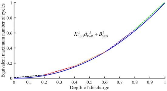
Figure 1.
Schematic diagram of piecewise linearization for the equivalent maximum number of cycles.
Equations (6) and (7) involve product terms between Boolean and continuous variables; such nonconvex nonlinear structures are difficult to directly incorporate into a linear optimization framework. For this reason, this paper linearizes the above formulas separately. For Equation (6), the original expression can be linearly relaxed and converted into an equivalent linear expression based on the logical dependence between variables, as shown in (9). For Equation (7), in order to deal with the product term between the mixed variables, this paper introduces the Big-M Method, which realizes the linear equivalent reconstruction of the constraints by constructing a set of auxiliary inequalities, and the corresponding linear constraints are in the form shown in (10). It should be noted that the Big-M method employed to linearize the product of a binary variable and a continuous term is an exact reformulation when M is sufficiently large. More specially, constraints (7) and (10) are algebraically equivalent: when the auxiliary binary = 1, the original relation holds exactly, and when = 0, , no further approximation is introduced by this reformulation.
where M is a positive real number with a sufficiently large value.
So far, an operation model of battery energy storage systems based on the rainfall-counting method has been constructed, which takes into account the loss of energy storage lifetime and is able to reduce this through the reasonable scheduling of energy storage to improve the economics of the distribution network’s operation.
2.2. Optimized Operational Model of an HNEDN Considering ESS Refinement Modeling
The optimal operation model of an HNEDN considering ESS refinement modeling aims to rationally dispatch distributed power sources, energy storage systems, and gas units in HNEDNs to reduce the system operation cost and increase the rate of new-energy consumption.
The objective function of the proposed model is to minimize the total operating cost, f, of HNEDNs, including the energy cost and the penalty cost for wind and light abandonment, as shown in (11).
where , , and are the unit prices of electricity, natural gas, and wind and light rejection penalties, respectively, at time t; and are the purchased power and natural gas volume, respectively, at time t; is the volume of natural gas consumed by the gas unit at time t; is the power of wind and light rejection of the HNEDN at time t; and and are the number of Gas Turbines (GTs) and Renewable Energy Sources (RESs), respectively, in the HNEDN.
The constraints of the proposed model include equipment operation constraints, power balance constraints, and power flow constraints. Specifically, the equipment operation constraints include ESS operation constraints, such as the service life losses shown in (1)–(8), and the operation constraints of GTs, wind turbines (WTs) [23], and PVs, which are are shown in (12)–(14) [24]; the power balance constraints are shown in (15) and (16); and the HNEDN trend constraints, based on the linear approximation of the AC tidal current method, are shown in (17)–(20).
where and are the GT electric power and the volume of natural gas consumed at time t, respectively; is the gas-to-electricity conversion coefficient of GT; , , and are the maximum values of the electric power of GT, WT, and PV, respectively; and are the electric power of WT and PV at time t, respectively; is the actual wind speed at time t; and , , and are the tangential, cut-out, and rated wind speeds, respectively; and are the efficiency and area of the PV module, respectively; is the light intensity at time t; is the renewable energy output at time t; is the electrical load power at time t; is the approximate auxiliary variable of ; k is the number of tangents to the approximate polyhedron of the cosine function; is the demand-responsive cut-load power at time t; and are the demand-responsive turnout and turn-in power at time t, respectively; is the safe range of the given phase angle (,); d is the spacing of the tangent points of the hyperplane tangents; is the nodal voltage deviation scalar value; and are the active and reactive power of line (i, j) at time t, respectively; is the voltage of the bus i at time t; and , , and are the conductance, conductivity, and phase angle of the line (i, j) at time t, respectively; and v = 1, 2, …, k are auxiliary scalars.
3. SDRO-Based Reconstruction and Linearization Method for the Optimal Operation Model of an HNEDN
3.1. Reconstruction Method of an HNEDN Optimal Operation Model Based on the Stochastic Distribution Robust Optimization Method
For the optimized operation model of an HNEDN described above, the high degree of uncertainty in both renewable energy output and load forecasting presents a critical challenge. Failure to address these uncertainties could render the resulting operation strategy impractical. Therefore, in this section, the source-load uncertainty is modeled using the Wasserstein distance and CVaR, and then the proposed model is reconstructed using the stochastic distribution robust optimization method to have the ability to cope with the source-load uncertainty.
For the new-energy output uncertainty, the output prediction error of the ith new-energy unit in the HNEDN is defined as . In practice, the true probability distribution of is usually difficult to determine, but the empirical probability distribution of can be obtained by extracting part of the probabilistic information about through Cartesian measures based on the limited historical data on prediction error, i.e., , as shown in (21). Then, a fuzzy set of probability distributions for the uncertainty of the new-energy outflow prediction error is established, centered on . In this paper, the Wasserstein distance is used to precisely measure the distance between and . Specifically, for two probability distributions, and , in a given tight support space , their Wasserstein distance can be expressed as (22). According to the previous definition, the fuzzy set of probability distributions of can be regarded as a Wasserstein ball with the empirical distribution as the center and as the radius, whose specific expression is shown in (23). can regulate the robustness of the optimization strategy, and is an important parameter in the distributional robust optimization framework, whose specific expression is shown in (24) and can be obtained using the dichotomy method.
where is the Cartesian measure of ; is the number of historical samples of new-energy output prediction errors; is the empirically distributed random variable; is the joint distribution function of and ; is the Wasserstein distance (1-norm) between the two random variables; is the confidence level of ; is an auxiliary variable; and is the average of the historical data of new-energy output prediction errors.
For load forecast uncertainty, this paper uses CVaR theory [25] to quantify the conditional value-at-risk of the HNEDN operating costs, taking into account load forecast uncertainty at a given confidence level. The expression for the loss function f resulting from load forecast uncertainty is first given as shown in (25). On this basis, the CVaR value of the HNEDN operating costs, considering load forecast uncertainty, can be obtained using (26).
where is the unit loss cost from the load forecast error at time t; and are the forecast and actual values of load at time t in scenario s, respectively; is the conditional value-at-risk of the HNEDN operating cost, taking into account the uncertainty of the load forecast; and is the value-at-risk of the HNEDN operating cost, which excludes the value of the cost loss after the occurrence of an extreme scenario as compared to ; is the number of typical operating scenarios for load forecasting; is the probability of the sth typical operating scenario occurring; denotes that the larger value of a and b is being used; is the confidence level; and is the HNEDN’s operating cost under scenario s, whose specific expression is shown in (11).
Based on the aforementioned modeling of HNEDN source-load uncertainty, the objective function after reconstruction based on SDRO is shown in (27). Specifically, in the first stage, where only new-energy output and load-demand forecast data are available, an initial optimized HNEDN operation strategy is developed to obtain the CVaR of the total HNEDN operation cost when considering the load forecast error scenario. In the second stage of real-time scheduling, a resource decision is made based on the actual data of new-energy output, and the reserved power of GT is invoked to smooth the power deviation generated by the uncertainty in the new-energy output prediction. It should be noted that GT is widely used for standby management due to its advantages of a fast response, high reliability, simplicity, flexibility, and controllability. Therefore, GT is selected in this paper to smooth the power deviation generated by the uncertainty in the new-energy output. It should be noted that the amount of natural gas consumed by the GT needs to be deducted from (11) because the operating cost of the GT is reflected in (27). In addition, the power deviation between the actual and planned output of the jth GT is equal to the power deviation caused by the prediction error in the new-energy output, as shown in (28).
where ,, and are the cost coefficients of the jth GT; is the actual power output of the jth GT at time t. denotes the mathematical expectation of the cost incurred by the GT to smooth the deviation of the predicted power for all the probability distribution scenarios, and is the decision variable of the power allocation coefficient of the jth GT at time t.
The source-load uncertainty of the HNEDN generates power deviations, which may cause the output power of the GT to exceed its safe operation range or the upper and lower backup limits, thus affecting the safe and stable operation of the HNEDN. Therefore, the reconfigured HNEDN optimized operation model needs to add the new distribution robust chance constraint presented in (29) to ensure that the GT can operate safely and stably within a certain probability range. Specifically, the first row constraint indicates that the probability that the output power of the ith GT is within its safe operation range is at least 1−; The second row constraint indicates that the probability that the new-energy power-deviation balance value assigned to the ith GT is within its standby power range is at least 1−.
where and are the upper and lower output power limits of the ith GT, respectively; is the upper reserve power limit of the ith GT; and are the confidence levels of the two distribution robust chance constraints, respectively.
3.2. Linearization of the HNEDN Optimized Operational Model Based on the Multiple Linearization Technique [26]
The above HNEDN optimization operation model is a non-convex nonlinear model, which is difficult to directly solve using commercial solvers.
Therefore, in this section, first, the mathematical expectation term shown in (27) is linearized using strong duality theory and the reconstructive linearization technique. On the basis of the coupling of (27) and (28), the defined auxiliary function f is used to replace the cost arising from the GT smoothing of the new-energy power deviation in the objective function. Then, according to the strong duality theory, the definite upper-bound mathematical expectation of the objective function can be equivalently converted to (30), with the three additional types of quadratic constraints shown in (31). For the three types of quadratic constraints shown in (31), the reconstructive linearization technique is used to convert them into the generic matrix expressions shown in (32). In order to express the reconstruction linearization process more clearly, an example of the first quadratic constraint in (31) is presented, which is equivalently converted to the internal elements of (32) and its sub-matrices , , , and (all m × n sub-matrices), i.e., , , , and , with the expressions shown in (33). The expressions of and are shown in (34).
where is a symmetric matrix; , , , and are auxiliary variables; .
Second, the two distributional robust chance constraints shown in (29) are also nonconvex nonlinear constraints, which are discussed in this section using the approximate linearized relaxation technique [27]. Firstly, the general form of the distributional robust chance constraints is presented, as shown in (35); then, (29) is collapsed into the general form of the distributional robust chance constraints shown in (35); and finally, the auxiliary continuous variables and are introduced and the distributional robust chance constraints of the general form are converted into the convex optimization constraints shown in (36) using the approximate linearized relaxation method.
where is the number of uncertain constraints; and are the equivalence coefficients of GT and uncertain constraints, respectively.
In addition, the constraint of ESS charging and discharging at different times, as presented in (3), can be relaxed, as demonstrated below. To analyze the charging of the ESS at a certain scheduling moment, two optimal charging strategies are assumed: one is that the ESS is charged with power while discharged with power , with > ; the other is that the ESS is charged with . These two charging strategies satisfy the constraints shown in (37). Equation (37) shows that both charging strategies can charge the ESS with the same electrical power at that scheduling moment. From the economic point of view, the charging cost of the first charging strategy is , while the charging cost of the second strategy is . Since the charging efficiency factor and the discharging efficiency factor of the ESS are both less than 1, the cost of the two associated charging strategies, as well as (37), can be obtained via (38). In Equation (38), the cost of the second charging strategy is shown to be lower than the first charging strategy. Since the objective function of the optimization model is to minimize the total operating cost of the HNEDN, the simultaneous charging and discharging shown in the first charging strategy will be excluded in the optimization search process to avoid additional charging costs. Similarly, the ESS discharge strategy will also exclude the simultaneous charging and discharging cases. Therefore, the not-simultaneous charging and discharging constraints shown in (3) can be relaxed.
So far, the HNEDN distribution robust optimization operation model considering a generalized energy storage support has been equivalently converted to a linear optimization model via the multiple linearization method, which can be mathematically modeled in the Yalmip platform of Matlab R2023a; the optimal solution can be obtained using the commercial solver Gurobi 11.0. The overall framework of the proposed SDRO-based operation approach is shown in Figure 2.
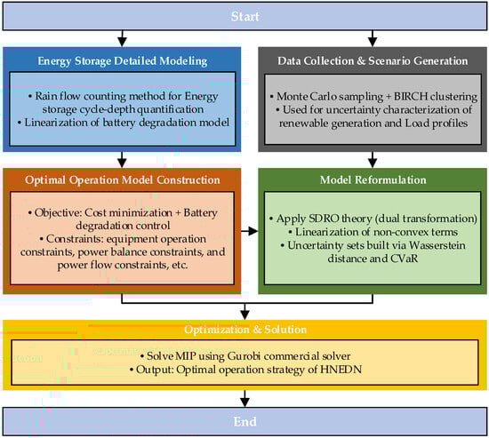
Figure 2.
Overall framework of the proposed SDRO-based operation approach.
4. Case Studies
In this paper, the modified IEEE 33-bus distribution system shown in Figure 3, which includes several wind and photovoltaic units, gas-fired units, and energy storage systems, is analyzed as an example. The Monte Carlo sampling method is used to generate a set of scenarios featuring prediction errors regarding the electric load and wind power of the HNEDN, which are superimposed on the historical data curves of load and wind power to obtain the initial operating scenarios for the electric load and wind power of the HNEDN. Then, the balanced iterative reducing and clustering using hierarchies (BIRCH) algorithm is used to reduce the scenarios to obtain the typical operating scenarios of renewable energy output and load demand of the improved IEEE-33 bus HNEDN, as shown in Figure 4. The main technical parameters of the algorithm in this paper are shown in Table 1. For other parameters, please refer to [21,24].
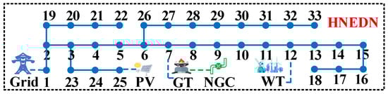
Figure 3.
Topological structure of the improved IEEE-33 bus HNEDN.
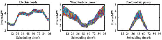
Figure 4.
Typical scenarios of renewable energy output and load demand of the improved IEEE-33 bus HNEDN.

Table 1.
Main technical parameters of the case study.
The optimal operation strategy of the HNEDN is shown in Figure 5, which depicts the actual dispatch outcomes of the HNEDN, including wind/PV utilization, demand response, and energy storage operation across the scheduling horizon. From Figure 5, it can be seen that the wind power and PV output occupied 91.3% of the total output in the whole dispatch cycle, which is a typical high-proportion new-energy distribution network. At moments 1~18, the HNEDN promoted new-energy consumption by storing 1.06 MW of energy and 0.42 MW of demand response due to the large wind power output and low load demand, but 11.63 MW of wind and PV was still abandoned. At points 30~54, at midday, the superimposed power of PV and wind power output far exceeded the load demand, so there was 15.33 MW of wind and solar power. At points 62~90, due to the low power output of new energy and the high load, both GT and the energy storage systems were discharged, and 2.1 MW was purchased from the grid to meet the peak load demand at this time. When using the above operation strategy, the overall new-energy consumption rate of HNEDN was 91.76%.
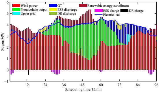
Figure 5.
Optimal operation strategy for HNEDN.
Figure 6 presents a comparison of the costs of the proposed strategy and the HNEDN optimization strategy without energy storage lifespan loss (S-WESL) [28]. As shown in Figure 6, since the strategy in this paper takes into account the lifetime loss of energy storage, it only discharges at critical moments, such as 20–26 and 68–74, to meet the new-energy consumption and load supply demands of HNEDN during the whole dispatch cycle, and the depth of discharging was limited to 70% of the total energy storage capacity. S-WESL aims to maximize economic benefits by greatly increasing the discharge depth of energy storage, with the maximum discharge depth reaching 80%. In addition, the average SOC of S-WESL in the whole dispatch cycle is only 1.09 MWh, while this paper used 1.66 MWh, which is a difference of 34%. Table 2 provides a comparison of the various costs obtained through paper’s strategy and S-WESL. Table 2 shows there were only 1.29 daily equivalent charge/discharge cycles in this strategy, and the corresponding service life of the energy storage was 3650 days, while the S-WESL strongly utilizes energy storage, so its daily equivalent charge/discharge cycles numbered 6.67, and the corresponding service life was only 705 days. The operating cost of S-WESL is USD 246 lower than this paper’s strategy when excluding the depreciation cost of energy storage, but the total operating cost of this paper’s strategy is 4.0% lower than that of S-WESL because its average daily depreciation cost of energy storage is USD 3149 higher than that of this paper’s model.
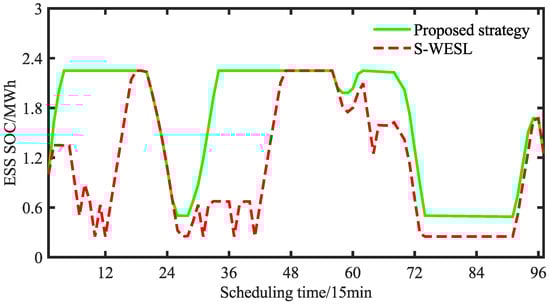
Figure 6.
Comparison between the proposed model and the S-WESL.
Table 2.
Comparison of various costs for the proposed model and the S-WESL.
Table 3 provides comparisons of the optimization results of the HNEDN under different storage capacities. In Table 3, it can be seen that the new-energy consumption rate of HNEDN increases gradually with the increase in distribution storage capacity. The increase in distribution storage capacity means that the average daily energy storage depreciation cost also increases, but the total operating cost of the HNEDN is reduced. However, the rate of increase in new-energy consumption and the rate of reduction in the total operating cost of the HNEDN gradually slows down with an increase in the allocated storage capacity. For example, when grows from 1.5 MWh to 2 MWh, the new-energy consumption rate of the HNEDN increases by 0.27% and the total operating cost decreases by 1.1%, while when grows from 3.5 MWh to 5 MWh, while the new-energy consumption rate of the HNEDN increases by only 0.12% and the total operating cost decreases by only 0.1%. Therefore, the decision-maker should consider the new-energy consumption rate, the cost of energy storage, the average daily depreciation cost of energy storage, and other factors in order to develop the most appropriate distribution program that considers the average daily depreciation cost of energy storage.
Table 3.
Solution results regarding optimized HNEDN operation with different distribution storage capacities.
To verify the advantages of SDRO compared to other uncertainty handling methods, Figure 7 presents the HNEDN operating costs, corresponding to different numbers representing historical samples for SDRO, DRO [29], RO [30], and SP [6], with β = 0.9. As can be seen from Figure 7, SP and RO make the most optimistic and conservative system operation strategies, respectively; the corresponding system operation costs are USD63,769 and USD76,558, respectively, and SP and RO are not able to utilize the information regarding uncertainty probability distributions provided by the historical samples, so they are not affected by the number of historical samples. The system operation costs of DRO are between those of SP and RO, but DRO uses Wasserstein distance to measure the Euclidean distance between the empirical distribution and the true distribution, so it can construct a suitable Wasserstein sphere based on the uncertainty probability distribution information provided by the new-energy output historical sample data, and then obtain a system operation strategy that considers the economy and robustness. The SDRO method used in this paper further uses CVaR to deal with the load forecast uncertainty based on DRO, which reduces the system’s operation costs by 2.36% on average compared with DRO for different numbers of historical samples, and further improves the system’s operation economy.
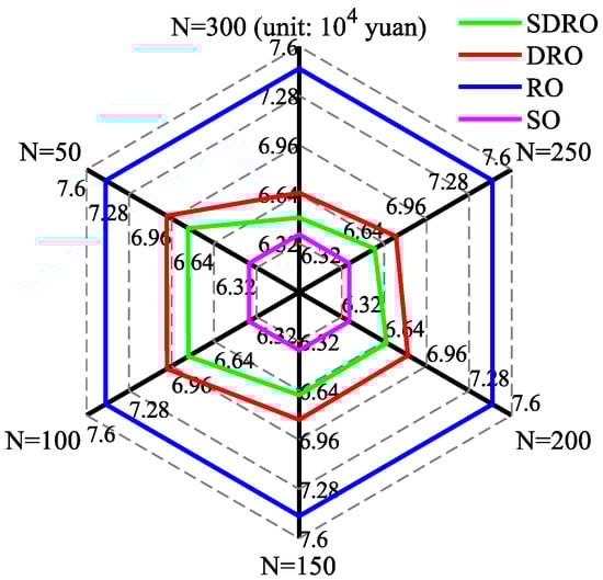
Figure 7.
Comparison of four uncertainty-handling methods.
In order to analyze the sensitivity of the distributional robust optimization method to changes in the confidence level and the number of available historical samples of new-energy output prediction errors, Figure 8 provides a comparison of the operating costs of the HNEDN for different scenarios, with different confidence levels (0.1~0.9) and different numbers of historical samples (Nsam = 50~300) of new-energy output prediction errors. Table 4 provides a comparison of the average radius of the Wasserstein sphere for different confidence level scenarios, with different numbers of historical samples of new-energy output prediction errors. Figure 8 and Table 4 show that the operating cost of HNEDN increases as the confidence level increases; this is because the higher the confidence level, the higher the requirement for HNEDN’s operational robustness, and the larger the radius of the probability distribution fuzzy ensemble sphere needs to be, based on the Wasserstein distance, to incorporate more and more extreme uncertainty scenarios. At this time, the resulting HNEDN operating strategy is more conservative, i.e., a certain amount of operating economy is sacrificed in exchange for higher operating robustness.
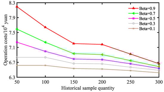
Figure 8.
Comparison of HNEDN operating costs under different confidence levels and with different amounts of historical data on renewable energy output prediction errors.
Table 4.
Comparison of Wasserstein sphere average radius under different confidence levels and historical data sizes for renewable energy output prediction errors.
Table 5 compares the time needed for the SDRO, DRO, RO, and SO methods with different historical sample or scenario sizes. It can be seen from Table 5 that the SDRO method requires the longest computation time due to the dual reformulation and the number of auxiliary variables introduced by the Wasserstein distance and CVaR modeling, which increased from 74 s at Nsam = 50 to 403 s at Nsam = 300. DRO shows a similar growth trend, with solving time rising from 69 s to 388 s, making it slightly faster than SDRO because its a simpler ambiguity structure. RO and SO feature two representative extreme settings: RO represents the most conservative case (smallest sample size and highest confidence level) and resolves it in 73 s, while SO corresponds to the most optimistic case (largest sample size and lowest risk aversion) and takes 399 s. While SDRO incurs the highest computational cost, it offers a favorable trade-off by delivering superior robustness and economic performance within an acceptable solving time.
Table 5.
Comparison of solving times for SDRO, DRO, RO, and SO methods with different historical sample or scenario sizes.
5. Conclusions
In this paper, a stochastic distributionally robust optimization operation method for a high-proportion new-energy distribution network, a considering detailed modeling of energy storage, is presented. Through arithmetic simulation, the following conclusions can be drawn:
- (1)
- The proposed HNEDN optimal operation method uses a detailed energy storage operation model. Compared to strategies that neglect energy storage life loss, the proposed strategy reduces battery energy storage system (BESS) life degradation, thereby lowering the average daily energy storage depreciation cost. This reduction leads to a 4.0% decrease in the total HNEDN operation cost.
- (2)
- The proposed SDRO method, using nested CVaR theory, was used to deal with the source-load uncertainty during system operation. Compared with stochastic planning and robust optimization methods, this method can adaptively adjust the economics and robustness of the HNEDN operation strategy according to the confidence level and the available historical sample data for new-energy output prediction errors; compared with the distributional robust optimization method, with a uniform modeling of the source-load uncertainty, this can ensure the robustness of the HNEDN operation and improve the HNEDN operation’s economics.
In future work, we will focus on applying the proposed method to larger-scale distribution networks to further verify its scalability and practicality. In addition, to improve its adaptability when using limited or biased data, the robustness of SDRO will be enhanced through data-denoising, scenario augmentation, and robust learning techniques.
Author Contributions
Conceptualization, B.L., D.Y. and C.C.; methodology, B.L. and Y.H.; formal analysis, B.L., Y.H. and D.Y.; investigation, Y.H.; writing—original draft, B.L. and C.C. visualization, C.F.; supervision, C.F. and C.C.; writing—review and editing, C.F. and C.C.; project administration, D.Y.; funding acquisition, D.Y. All authors have read and agreed to the published version of the manuscript.
Funding
This work was funded by the Science and Technology Project of State Grid Fujian Electric Power Co., Ltd. (No. 52136024000P).
Data Availability Statement
The original contributions presented in this study are included in the article. Further inquiries can be directed to the corresponding author.
Conflicts of Interest
Authors Bin Lin and Yan Huang were employed by State Grid Longyan Power Supply Company of Fujian Electric Power Co., Ltd. Author Dingwen Yu was employed by State Grid Fujian Economic and Technology Research Institute. The remain authors declare that the research was conducted in the absence of any commercial or financial relationship that could be construed as a potential conflict of interest.
Nomenclature
| Abbreviations | |
| HNEDN | High-proportion new-energy distribution network |
| CvaR | Conditional value at risk |
| SP | Stochastic programming |
| RO/DRO/SDRO | Robust optimization/distributed robust optimization/stochastic distributed robust optimization |
| PV | Photovoltaic |
| DG | Distributed generator |
| ESS/RES | Energy storage systems/renewable energy source |
| SOC | State of charge |
| DR/DSR | Demand response/demand side response |
| DoD | Depth of discharge |
| GT/WT | Gas turbine/wind turbine |
| BIRCH | Balanced iterative reducing and clustering using hierarchies |
| S-WESL | Strategy without energy storage lifespan loss |
| Variables | |
| State of charge of the ESS at time t | |
| Charging powers of the ESS at time t | |
| / | Charging/discharging quantities of the ESS at time t |
| Auxiliary Boolean variables | |
| Discharge depth of the ESS at time t | |
| / | Maximum charge and discharge cycles with /100% discharge depth each time |
| Auxiliary Boolean variable | |
| / | Slope and intercept of each segment |
| Auxiliary Boolean variable reflecting the state of the ESS charge/discharge cycle at time t | |
| / | Purchased power and natural gas volume at time t |
| Volume of natural gas consumed by the gas unit at time t | |
| Power of wind and light rejection at time t | |
| / | Electric power of WT/PV at time t |
| Actual wind speed at time t | |
| Light intensity at time t | |
| / | Renewable energy output/electrical load power at time t |
| Approximate auxiliary variable | |
| // | Demand-responsive cut-load/turnout/turn-in power at time t |
| Nodal voltage deviation scalar value | |
| / | Active and reactive power of the line (i, j) at time t |
| Voltage of the bus i at time t | |
| // | Conductance/conductivity/phase angle of the line (i, j) at time t |
| / | ith new-energy unit/the empirically distributed random variable |
| Cartesian measure of | |
| Number of historical samples of new-energy output prediction error | |
| The Wasserstein distance (1-norm) between the two random variables | |
| Confidence level of | |
| Auxiliary variable | |
| Average of the historical data of new-energy output prediction error | |
| Unit loss cost from the load forecast error at time t | |
| / | Forecast and actual values of load at time t in scenario s |
| / | Value-at-risk/the conditional value-at-risk of the HNEDN operating cost |
| Operating cost under scenario s | |
| Actual power output of the jth GT at time t | |
| Mathematical expectation of the cost | |
| Decision variable of the power allocation coefficient of the jth GT at time t | |
| /// | Auxiliary variables |
| / | Equivalence coefficients of GT and uncertain constraints |
| Symmetric matrix | |
| Constant | |
| / | Upper and lower limits of the SOC of the ESS |
| // | Self-depletion coefficients/charging loss coefficients/discharging loss coefficients of the ESS |
| Time interval between neighboring dispatch moments | |
| / | Actual/standard number of cycles |
| Fitting parameter | |
| / | Upper and lower limits of the discharge depth of the kth segment |
| Maximum daily average number of charge and discharge cycles | |
| Expected service lives of the ESS | |
| M | Positive real number with a sufficiently large value |
| // | Unit price of electricity, natural gas price, and the unit price of wind and light rejection penalties at time t |
| / | Number of Gas Turbines/Renewable Energy Sources |
| Gas-to-electricity conversion coefficient of GT | |
| // | Maximum values of the electric power of GT/WT/PV |
| // | Tangential/cut-out/rated wind speeds |
| / | Efficiency and area of the PV module |
| k | Number of tangents to the approximate polyhedron of the cosine function |
| Safe range of the given phase angle | |
| v | Auxiliary scalars |
| Number of typical operating scenarios for load forecasting | |
| Probability of the sth typical operating scenario occurring | |
| Confidence level | |
| // | Cost coefficients of the jth GT |
| // | Upper/the upper-reserve/the lower-output power limits of the ith GT |
| / | Confidence levels of the two distribution robust chance constraints |
| Number of uncertain constraints |
References
- Wang, G.; Wang, C.; Feng, T.; Wang, K.; Yao, W.; Zhang, Z. Day-Ahead and Intraday Joint Optimal Dispatch in Active Distribution Network Considering Centralized and Distributed Energy Storage Coordination. IEEE Trans. Ind. Appl. 2024, 60, 4832–4842. [Google Scholar] [CrossRef]
- Gan, W.; Ai, X.; Fang, J.; Yan, M.; Yao, W.; Zuo, W.; Wen, J. Security constrained co-planning of transmission expansion and energy storage. Appl. Energy 2019, 239, 383–394. [Google Scholar] [CrossRef]
- Liu, J.; Sun, K.; Ding, Z.; Li, K.J.; Sun, Y. Multi-stage planning of distribution network with high penetration renewable energy considering reliability index. IEEE Trans. Ind. Appl. 2023, 60, 2344–2356. [Google Scholar] [CrossRef]
- Liao, J.; Lin, J.; Wu, G.; Lai, S. Collaborative Optimization Planning Method for Distribution Network Considering “Hydropower, Photovoltaic, Storage and Charging”. IEEE Access 2024, 12, 172115–172124. [Google Scholar] [CrossRef]
- Chen, W.; Hao, P.; Wei, Z.; Chen, L. Study on the optimization allocation method of distributed energy storage in an active distribution network taking into account transmission betweenness and source-network-load synergy. Electr. Power Syst. Res. 2025, 247, 111787. [Google Scholar] [CrossRef]
- Ding, T.; Qu, M.; Huang, C.; Wang, Z.; Du, P.; Shahidehpour, M. Multi-period active distribution network planning using multi-stage stochastic programming and nested decomposition by SDDIP. IEEE Trans. Power Syst. 2020, 36, 2281–2292. [Google Scholar] [CrossRef]
- Zhao, B.; Ren, J.; Chen, J.; Lin, D.; Qin, R. Tri-level robust planning-operation co-optimization of distributed energy storage in distribution networks with high PV penetration. Appl. Energy 2020, 279, 115768. [Google Scholar] [CrossRef]
- Baharvandi, A.; Aghaei, J.; Nikoobakht, A.; Niknam, T.; Vahidinasab, V.; Giaouris, D.; Taylor, P. Linearized hybrid stochastic/robust scheduling of active distribution networks encompassing PVs. IEEE Trans. Smart Grid 2019, 11, 357–367. [Google Scholar] [CrossRef]
- Zhu, J.; Huang, Y.; Lu, S.; Shen, M.; Yuan, Y. Incorporating local uncertainty management into distribution system planning: An adaptive robust optimization approach. Appl. Energy 2024, 363, 123103. [Google Scholar] [CrossRef]
- Wu, M.; Kou, L.; Hou, X.; Ji, Y.; Xu, B.; Gao, H. A bi-level robust planning model for active distribution networks considering uncertainties of renewable energies. Int. J. Electr. Power Energy Syst. 2019, 105, 814–822. [Google Scholar] [CrossRef]
- Sheng, H.; Wang, C.; Li, B.; Liang, J.; Yang, M.; Dong, Y. Multi-timescale active distribution network scheduling considering demand response and user comprehensive satisfaction. IEEE Trans. Ind. Appl. 2021, 57, 1995–2005. [Google Scholar] [CrossRef]
- Nejad, B.M.; Vahedi, M.; Hoseina, M.; Moghaddam, M.S. Economic model for coordinating large-scale energy storage power plant with demand response management options in smart grid energy management. IEEE Access 2022, 11, 16483–16492. [Google Scholar] [CrossRef]
- Liu, H.; Wang, Z. Research on energy storage and high proportion of renewable energy planning considering demand. IEEE Access 2020, 8, 198591–198599. [Google Scholar] [CrossRef]
- Khani, M.; Moghaddam, M.S.; Noori, T.; Ebrahimi, R. Integrated energy management for enhanced grid flexibility: Optimizing renewable resources and energy storage systems across transmission and distribution networks. Heliyon 2024, 10, 39585. [Google Scholar] [CrossRef] [PubMed]
- Ren, Z.; Guo, H.; Yang, P.; Zuo, G.; Zhao, Z. Bi-level optimal allocation of flexible resources for distribution network considering different energy storage operation strategies in electricity market. IEEE Access 2020, 8, 58497–58508. [Google Scholar] [CrossRef]
- Azizivahed, A.; Arefi, A.; Ghavidel, S.; Shafie-Khah, M.; Li, L.; Zhang, J.; Catalão, J.P. Energy management strategy in dynamic distribution network reconfiguration considering renewable energy resources and storage. IEEE Trans. Sustain. Energy 2019, 11, 662–673. [Google Scholar] [CrossRef]
- Wang, J.; Xie, N.; Huang, C.; Wang, Y. Two-stage stochastic-robust model for the self-scheduling problem of an aggregator participating in energy and reserve markets. Prot. Control. Mod. Power Syst. 2023, 8, 1–20. [Google Scholar] [CrossRef]
- Dong, Z.Y.; Zhang, Z.; Zhang, R.; Wang, T. Battery Doctor-next generation battery health assessment: Definition, approaches, challenges and opportunities. Energy Convers. Econ. 2023, 4, 417–424. [Google Scholar] [CrossRef]
- Sioshansi, R.; Denholm, P.; Arteaga, J.; Awara, S.; Bhattacharjee, S.; Botterud, A.; Cole, W.; Cortés, A.; De Queiroz, A.; DeCarolis, J.; et al. Energy-storage modeling: State-of-the-art and future research directions. IEEE Trans. Power Syst. 2021, 37, 860–875. [Google Scholar] [CrossRef]
- Alharbi, H.; Bhattacharya, K. Stochastic optimal planning of battery energy storage systems for isolated microgrids. IEEE Trans. Sustain. Energy 2018, 9, 211–227. [Google Scholar] [CrossRef]
- Andrenacci, N.; Chiodo, E.; Lauria, D.; Mottola, F. Life cycle estimation of battery energy storage systems for primary frequency regulation. Energies 2018, 11, 3320. [Google Scholar] [CrossRef]
- He, Q.; Chen, C.; Fu, X.; Yu, S.; Wang, L.; Lin, Z. Joint planning method of shared energy storage and multi-energy microgrids based on dynamic game with perfect information. Energies 2024, 17, 4792. [Google Scholar] [CrossRef]
- Verma, N.; Kumar, N.; Gupta, S.; Malik, H.; Márquez, F.P.G. Review of sub-synchronous interaction in wind integrated power systems: Classification, challenges, and mitigation techniques. Prot. Control Mod. Power Syst. 2023, 8, 1–26. [Google Scholar] [CrossRef]
- Liu, H.; Li, H.; Liu, H.; Gu, C.; Li, Q.; Ren, Q. A closed-loop representative day selection framework for generation and transmission expansion planning with demand response. Energy Convers. Econ. 2024, 5, 93–109. [Google Scholar] [CrossRef]
- Zhang, Q.; Leng, S.; Ma, X.; Liu, Q.; Wang, X.; Liang, B.; Liu, Y.; Yang, J. CVaR-constrained policy optimization for safe reinforcement learning. IEEE Trans. Neural Netw. Learn. Syst. 2024, 36, 830–841. [Google Scholar] [CrossRef] [PubMed]
- Chen, C.; Wu, X.; Li, Y.; Zhu, X.; Li, Z.; Ma, J.; Qiu, W.; Liu, C.; Lin, Z.; Yang, L.; et al. Distributionally robust day-ahead scheduling of park-level integrated energy system considering generalized energy storages. Appl. Energy 2021, 302, 117493. [Google Scholar] [CrossRef]
- Zhou, A.; Yang, M.; Wang, M.; Zhang, Y. A linear programming approximation of distributionally robust chance-constrained dispatch with Wasserstein distance. IEEE Trans. Power Syst. 2020, 35, 3366–3377. [Google Scholar] [CrossRef]
- Ma, M.; Huang, H.; Song, X.; Peña-Mora, F.; Zhang, Z.; Chen, J. Optimal sizing and operations of shared energy storage systems in distribution networks: A bi-level programming approach. Appl. Energy 2022, 307, 118170. [Google Scholar] [CrossRef]
- Ma, M.; Long, Z.; Liu, X.; Lee, K.Y. Distributionally robust optimization of electric-thermal-hydrogen integrated energy system considering source-load uncertainty. Energy 2025, 316, 134568. [Google Scholar] [CrossRef]
- Jeddi, B.; Vahidinasab, V.; Ramezanpour, P.; Aghaei, J.; Shafie-khah, M.; Catalão, J.P. Robust optimization framework for dynamic distributed energy resources planning in distribution networks. Int. J. Electr. Power Energy Syst. 2019, 110, 419–433. [Google Scholar] [CrossRef]
Disclaimer/Publisher’s Note: The statements, opinions and data contained in all publications are solely those of the individual author(s) and contributor(s) and not of MDPI and/or the editor(s). MDPI and/or the editor(s) disclaim responsibility for any injury to people or property resulting from any ideas, methods, instructions or products referred to in the content. |
© 2025 by the authors. Licensee MDPI, Basel, Switzerland. This article is an open access article distributed under the terms and conditions of the Creative Commons Attribution (CC BY) license (https://creativecommons.org/licenses/by/4.0/).