Discrete-Time Internal Model Control with Equal-Order Fractional Butterworth Filter for Multivariable Systems

Abstract

A novel discrete-time internal model control (IMC) method cascaded with a discrete-time equal-order fractional Butterworth (EFBW) filter is proposed for multivariable systems with time-delay and non-minimum-phase (NMP) zeros. This is the first attempt to design such a control scheme in the discrete-time domain, as previous work has typically focused on continuous-time systems. An inverted decoupling (ID) method is introduced and integrated with the discrete-time IMC controller, forming a discrete-time ID-IMC scheme that mitigates coupling effects among control loops. Additionally, a discrete-time EFBW filter is designed to balance flexibility and design complexity effectively, with technical specifications guiding the determination of the filter’s optimal order. Structured singular value analysis is conducted to guarantee the stability and robustness of the resulting closed-loop system. Illustrative examples are provided, demonstrating the effectiveness and advantages of the proposed control method.

1. Introduction

The internal model control (IMC), a sophisticated model-based control strategy pioneered by Morari and his co-workers [1,2], is widely applied in chemical process control. The IMC technique provides a convenient structure for not only avoiding the design complexity of the control system but also achieving a good trade-off between the closed-loop performance and robustness [3,4]. Therefore, the IMC approach has been widely discussed (see refs. [1,2,3,4,5,6,7,8,9,10,11,12,13,14,15] for more details). For linear multivariable systems, the IMC scheme offers a practical inverse controller that can approximate desired closed-loop performance, even in the presence of time-delay and non-minimum-phase (NMP) zeros [13].

Selecting an appropriate IMC filter is crucial for the IMC-based controller design to enhance system robustness against external disturbances or model uncertainties [2,3,13,14,15]. Ogunba et al. [14] proposed a decoupling IMC method for multivariable stable processes with time-delays and NMP zeros, such that achieved the decoupling and improved the closed-loop performance. In the presence of disturbances and process uncertainties, Kumar et al. [15] introduced a modified two-degrees-of-freedom IMC based on the maximum peak gain margin stability criteria to address weaknesses in the presence of disturbances and process uncertainties. The authors in refs. [16,17] added conventional diagonal low-pass filters into the feedback loop to ensure the robustness of control systems. Subsequently, many IMC filter optimization methods, such as non-diagonal filter [18], lead-lag filter [19], and Butterworth (BW) filter [20], were developed to further enhance the robustness and improve disturbance rejection ability.

In addition, fractional-order (FO) design methods offer significant advantages over traditional integer-order (IO) methods in modeling and control applications. They provide greater flexibility and possess infinite memory, enabling more precise dynamical descriptions with fewer parameters [21,22]. Leveraging the advantages of the FO design, the IMC has been extended to develop FO-IMC schemes. References [19,21,22] introduced a FO-IMC design based on the PID structure, which combines an IO PID controller with a FO filter. This design was later adapted for multiple-input-multiple-output (MIMO) systems in [23,24], which offers enhanced flexibility in controller and filter design, along with more adjustable time and frequency responses, thus achieving a robust performance. For IO processes with time-delay, Li et al. [7] proposed a FO-IMC controller based on a FO filter, which surpassed the IO filters in robustness and design flexibility. Further, a two-degrees-of-freedom FO-IMC controller was designed for FO systems with time-delay by Gnaneshwar et al. [25]; the set-point tracking and robustness can be adjusted by the tunable parameters of the controller directly.

Note that the aforementioned works for multivariable systems were designed in the continuous-time domain, which in fact, needs to be discretized for practical applications [26]. With the widespread use of computers and microprocessors in modern industrial engineering, the discrete-time IMC design method is crucial for enhancing control effectiveness and boosting productivity [3]. However, discrete-time IMC schemes have been rarely explored, with only a few studies available [1,2,8,9,26]. Garcia et al. [1] first introduced the discrete-time IMC for single-input-single-output (SISO) systems, and later extended it to MIMO systems [2]. Until recently, a discrete-time IMC controller for industrial processes with time-delay was proposed by a few authors [8,9]. Silva et al. [10] developed a novel discrete-time adaptive IMC, which was robust to changes in modeling by minimizing the performance index. For MIMO systems, modified discrete-time IMC techniques were proposed by refs. [11,12]. Typically, the discrete-time IMC controller is often augmented with a discrete-time IMC filter, primarily for the purpose of achieving an optimal compromise between the set-point tracking and robustness [27].

It is also important to mention that the tuning rules of the above literature incorporate a classical low-pass IMC filter with fewer tunable parameters, which limits flexibility and performance. Furthermore, few of these studies have focused on discrete-time IMC schemes for MIMO processes with multiple time-delays and NMP zeros. In this study, we propose a novel discrete-time IMC controller based on inverted decoupling (ID) for MIMO processes, considering multiple time-delays and NMP zeros. To ensure closed-loop realizability and enhance system performance, a discrete-time ID-IMC controller with a cascaded FO filter is designed, replacing the traditional IO filter. While traditional BW filter approximations, which have no ripple in the pass band or the stop band [28,29], could be employed to construct a FO Butterworth (FOBW) filter with more flexibility, however, the tuning of the filter would be much more complex. Therefore, an equal-order fractional BW (EFBW) filter is adopted to simplify the tuning and further discretized in the discrete-time domain. Indeed, the design in the discrete-time domain is quite different numerically from its continuous-time counterpart. An efficient discretization algorithm based on interpolations between Tustin’s and Euler’s methods [30] is proposed to create the discrete-time EFBW filter, which exactly preserves the stability domain and avoids complex impulse response calculations. To the best of our knowledge, this is the first study to combine an EFBW filter with an IMC controller in the discrete-time domain. In practice, the proposed control scheme also provides an acceptable trade-off between process magnitude and phase through filter parameter tuning.

The rest of this paper is structured as follows: Section 2 derives the general expressions for multivariable systems using the discrete-time ID-IMC controller and discusses conditions for system physical realizability. In Section 3, the traditional IMC filter is modified as an EFBW filter in the discrete-time domain, and then integrated with the ID-IMC controller. Section 4 and Section 5 provide stability and robustness analyses of the proposed scheme. Simulation examples are presented in Section 6 to illustrate the effectiveness of the proposed method. Finally, Section 7 provides the conclusion of this paper.

2. Discrete-Time Internal Model Control with Inverted Decoupling

2.1. Structure of the Discrete-Time ID-IMC

Let $P\left(z\right)={\left[p_{ij}\right]}_{n\times n}$, $i,j=1,2,\dots ,n$ denote the controlled process matrix with $n$ inputs and $n$ outputs, and ${\mathit{P}}_{\mathrm{m}}\left(z\right)$ represents the discrete-time transfer matrix of the process model. In order to decrease the sensitivity to uncertainties and enhance the robustness to disturbances, the general IMC structure is applied, as illustrated in Figure 1.

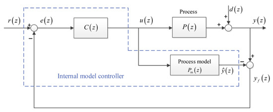
Figure 1. The IMC structure.

Given that the controlled process $P\left(z\right)$ exhibits a $n\times n$ MIMO structure with significant coupling between inputs and outputs, to mitigate the effect of the couplings and simplify parameter tuning for achieving desired performance indicators, it is necessary to decouple $P\left(z\right)$. Common decoupling methods include ideal decoupling [31], simple decoupling [32,33,34,35], and inverted decoupling (ID) [36,37,38,39]. Notably, as the ID integrates the advantages of the other two approaches [40,41], an Inverse Decoupling-based Internal Model Control (ID-IMC) structure is adopted, as illustrated in Figure 2, where $C\left(z\right)$ includes a discrete-time forward channel matrix $C_{\mathrm{d}}\left(z\right)$ and a feedback channel matrix $C_{\mathrm{o}}\left(z\right)$, which will achieve precise decoupling and ensure robust system stability, enabling the system output $y\left(z\right)$ to accurately track the reference signal $r\left(z\right)$ in the presence of time-delay, model uncertainties, and external disturbances $d\left(z\right)$.

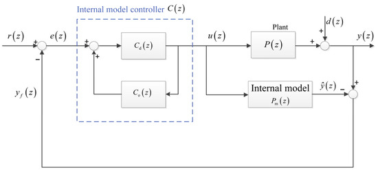
Figure 2. The discrete-time ID-IMC structure.

Applying the ID structure yields

$$C\left(z\right)={\left[I-C_{\mathrm{d}}\left(z\right)C_{\mathrm{o}}\left(z\right)\right]}^{-1}{C}_{\mathrm{d}}\left(z\right)$$

(1)

Then the control task is converted to design the decoupling matrices $C_{\mathrm{d}}\left(z\right)$ and $C_{\mathrm{o}}\left(z\right)$.

2.2. Design of $C_{\mathrm{d}}\left(z\right)$ and $C_{\mathrm{o}}\left(z\right)$

The input and output transfer matrix derived from Figure 2 is

$$y\left(z\right)=d\left(z\right)+P\left(z\right){\left[I+C\left(z\right)\left(P\left(z\right)-P_m\left(z\right)\right)\right]}^{-1}C\left(z\right)\left(r\left(z\right)-d\left(z\right)\right)$$

(2)

According to the design concept of the IMC, it is first assumed that the model is matched, i.e., $P_{\mathrm{m}}\left(z\right)=P\left(z\right)$, by which Equation (2) becomes

$$y\left(z\right)=P\left(z\right)C\left(z\right)r\left(z\right)+\left(I-P\left(z\right)C\left(z\right)\right)d\left(z\right)$$

(3)

From Figure 2, the closed-loop transfer matrix of the discrete-time system can be derived as $T\left(z\right)\triangleq y\left(z\right)/r\left(z\right)=P\left(z\right)C\left(z\right){\left[I+\left(P\left(z\right)-P_{\mathrm{m}}\left(z\right)\right)C\left(z\right)\right]}^{-1}$, which reduces to $T\left(z\right)=P\left(z\right)C\left(z\right)=\mathrm{diag}\left(t_1\left(z\right),t_2\left(z\right),\dots ,t_n\left(z\right)\right)$ under the conditions $P\left(z\right)=P_{\mathrm{m}}\left(z\right)$ and $d=0$. Using Equation (1), the following expression can be obtained:

$$C_{\mathrm{d}}^{-1}\left(z\right)-C_{\mathrm{o}}\left(z\right)=T^{-1}\left(z\right)P\left(z\right)$$

(4)

which is expanded as

$$\left[\begin{array}{cccc}{\displaystyle \frac{1}{c_{{\mathrm{d}}_{11}}}}& -c_{{\mathrm{o}}_{12}}& \dots & -c_{{\mathrm{o}}_{1n}}\\ -c_{{\mathrm{o}}_{21}}& {\displaystyle \frac{1}{c_{{\mathrm{d}}_{22}}}}& \dots & -c_{{\mathrm{o}}_{2n}}\\ ⋮& ⋮& \ddots & ⋮\\ -c_{{\mathrm{o}}_{n1}}& -c_{{\mathrm{o}}_{n2}}& \dots & {\displaystyle \frac{1}{c_{{\mathrm{d}}_{nn}}}}\end{array}\right]=\left[\begin{array}{cccc}{\displaystyle \frac{p_{11}}{t_1}}& {\displaystyle \frac{p_{12}}{t_1}}& \dots & {\displaystyle \frac{p_{1n}}{t_1}}\\ {\displaystyle \frac{p_{21}}{t_2}}& {\displaystyle \frac{p_{22}}{t_2}}& \ddots & {\displaystyle \frac{p_{2n}}{t_2}}\\ ⋮& ⋮& \ddots & ⋮\\ {\displaystyle \frac{p_{n1}}{t_n}}& {\displaystyle \frac{p_{n2}}{t_n}}& \dots & {\displaystyle \frac{p_{nn}}{t_n}}\end{array}\right]$$

(5)

Given that $C\left(z\right)$ establishes a one-to-one mapping between $e\left(z\right)$ and $u\left(z\right)$, it means $C_{\mathrm{d}}\left(z\right)$ must have only $n$ non-zero element that connects the system error $e\left(z\right)$ and controller output $u\left(z\right)$. In addition, since $C_{\mathrm{o}}\left(z\right)$ feeds back $u\left(z\right)$ towards the controller input, it must have only $n$ zero element corresponding to $C_{\mathrm{d}}\left(z\right)$.

Note that $C_{\mathrm{d}}\left(z\right)$ has to be non-singular since it is inverted; when its non-zero elements are chosen, they are distributed exclusively in each row and column. Therefore, for $n\times n$ square multivariable systems, there are $n!$ possible configurations for $C_{\mathrm{d}}\left(z\right)$ and $C_{\mathrm{o}}\left(z\right)$, including the matrix form, as seen in Equation (5). For the $i$-th row of $C_{\mathrm{d}}\left(z\right)$, let the position of the non-zero element be $q_i$, according to the ID technique [41], and $C_{\mathrm{d}}\left(z\right)$ and $C_{\mathrm{o}}\left(z\right)$ can be given as

$$c_{{\mathrm{d}}_{ij}}\left(z\right)=\left\{\begin{array}{l}{\displaystyle \frac{t_j\left(z\right)}{p_{ji}\left(z\right)}}, \forall i; j=q_i\\ 0,\hspace{1em}\hspace{1em}\hspace{1em}\mathrm{otherwise}. \end{array}\right.$$

(6)

$$c_{{\mathrm{o}}_{ij}}\left(z\right)=\left\{\begin{array}{l}-{\displaystyle \frac{p_{ij}\left(z\right)}{t_i\left(z\right)}}, \forall i,j;\hspace{0.17em} i\ne q_i\\ 0,\hspace{1em}\hspace{1em}\hspace{1em}\mathrm{otherwise}. \end{array}\right.$$

(7)

Compared with the conventional multivariable decoupling IMC, the main advantage of the ID-IMC is its computational simplicity, regardless of the size of the system, because each row of Equation (4) contains only one value to be calculated for each position.

2.3. Realizability and the Closed-Loop Performance

However, it is often impossible to achieve an exact match between models. Furthermore, the vast majority of industrial processes inherently involve time-delay and NMP zeros, which may result in non-causal and unstable poles during model inversion according to Equation (6). To tackle these challenges, only the causal and minimum-phase components can be inverted, thereby leading to the realizability problem. For a physically realizable ID-IMC controller, $C_{\mathrm{d}}\left(z\right)$ and $C_{\mathrm{o}}\left(z\right)$ must satisfy the following criteria.

• Stability. The controller must generate a bounded response to bounded inputs; therefore, all poles of $C_{\mathrm{d}}\left(z\right)$ and $C_{\mathrm{o}}\left(z\right)$ must lie inside the unit circle of the z-plane;
• Causality. The controller must be causal, which means that the controller must make no prediction;
• Properness. A strictly proper transfer function has a denominator order equal to/greater than the numerator order.

2.3.1. Multiple Time-Delays

Let the plant transfer matrix $P\left(z\right)$ with multiple time-delay terms have the following form:

$$P\left(z\right)=\left[\begin{array}{cccc}{z}^{-{\tau }_{11}}{p\prime }_{11}\left(z\right)& z^{-{\tau }_{12}}{p\prime }_{12}\left(z\right)& \dots & z^{-{\tau }_{1n}}{p\prime }_{1n}\left(z\right)\\ z^{-{\tau }_{21}}{p\prime }_{21}\left(z\right)& z^{-{\tau }_{22}}{p\prime }_{22}\left(z\right)& \dots & z^{-{\tau }_{2n}}{p\prime }_{2n}\left(z\right)\\ ⋮& ⋮& ⋮& ⋮\\ z^{-{\tau }_{n1}}{p\prime }_{n1}\left(z\right)& z^{-{\tau }_{n2}}{p\prime }_{n2}\left(z\right)& \dots & z^{-{\tau }_{\mathit{nn}}}{p\prime }_{\mathit{nn}}\left(z\right)\end{array}\right]$$

(8)

i.e., $P\left(z\right)={\left[p_{ij}\left(z\right)\right]}_{n\times n}\triangleq {\left[z^{-{\tau }_{ij}}{p\prime }_{ij}\left(z\right)\right]}_{n\times n}$, $i,j=1,2,\dots ,n$, in which the positive integer ${\tau }_{ij}$ is the time-delay of each element $p_{ij}\left(z\right)$. For the $i$-th row of $P\left(z\right)$, if $p_{ik}\left(z\right)$, $\mathrm{k}=1,2,\dots ,n$ is a transfer function of the $k$-th column with the minimum time-delay ${\tau }_{ik}$, and the time-delay ${\tau }_i$ specification of the desired closed-loop transfer function $t_i\left(z\right)$ must satisfy

$${\tau }_{ik}<{\tau }_i=\max \left({\tau }_{ij}\right),\forall i,j$$

(9)

which yields the biggest time-delay in each output response, such that the realizability of causality can be guaranteed for the desired closed-loop transfer matrix $T\left(z\right)$ according to Equations (6) and (7).

2.3.2. Zeros Outside the Unit Circle

Note that $C_{\mathrm{d}}\left(z\right)$ and $C_{\mathrm{o}}\left(z\right)$ should be stable, implying that the inverse of $t_i\left(z\right)$ and $p_{ij}\left(z\right)$ should be stable from Equations (6) and (7); therefore, $t_i\left(z\right)$ should be carefully selected based on the zeros of $P\left(z\right)$. Let ${\sigma }_x, \left(x=1,2,\dots ,N\right)$ be the unstable zeros of $P\left(z\right)$ outside the unit circle, let $N$ be the multiplicity of the unstable zeros, and define ${\upsilon }_{ik}$ as the smallest zero multiplicity outside the unit circle of row $i$. The zero multiplicity ${\upsilon }_i$ outside the unit circle of the closed-loop transfer function $t_i\left(z\right)$ of row $i$ should be chosen as

$${\upsilon }_{ik}<{\upsilon }_i=\min \left({\upsilon }_{ij}\right), \forall i,j$$

(10)

such that the inverse of $t_i\left(z\right)$ and $p_{ij}\left(z\right)$ defined by Equations (6) and (7) are stable.

Therefore, Section 2.3.1 and Section 2.3.2 discussed the realizable conditions for achieving a rational desired closed-loop transfer matrix $T\left(z\right)$; thereby, $t_i\left(z\right)$ should be suggested as a transfer function with the minimum time-delay and smallest zero multiplicity outside the unit circle given by

$$t_i\left(z\right)=z^{-{\tau }_i}\prod _{x=1}^N{\left[{\displaystyle \frac{z-{\sigma }_x}{z-{\widehat{\sigma }}_x}}\right]}^{{\upsilon }_i}\overline{H}\left(z\right)$$

(11)

where ${\sigma }_x$ is the zeros of $P\left(z\right)$, and ${\widehat{\sigma }}_x$ is their images inside the unit circle, which meet

$${\widehat{\sigma }}_x=\left\{\begin{array}{c}{\sigma }_x,\hspace{1em}\left|{\sigma }_x\right|\le 1\\ {\displaystyle \frac{1}{{\sigma }_x}},\hspace{1em}\left|{\sigma }_x\right|>1\end{array}\right.$$

(12)

and $\overline{H}\left(z\right)$ is the low-pass EFBW filter to be designed to enhance the robustness.

3. Discrete-Time Equal-Order Fractional Butterworth Filter

It is worth noting that the model exhibits a mismatch. Specifically, the IMC structure depicted in Figure 1 does not represent an open-loop configuration. If the model mismatch remains uncompensated, it could degrade the system performance and potentially lead to instability. Consequently, a filter must be cascaded to enhance the robustness of the system. It should be emphasized that, in most industrial processes, the order of the IMC filter is typically restricted to integer values (primarily first-order or second-order), which limits both flexibility and robustness. By contrast, fractional-order (FO) filters are more appealing than integer-order (IO) ones due to their superior robustness properties and additional degrees of freedom for meeting design specifications [19].

In this section, a novel discrete-time EFBW filter is added to the discrete-time ID-IMC system, whose response in discrete-time domain is approximated using fractional calculus. The proposed filter decreases the tunable parameters for proper degrees of freedom with a simplified structure compared with the FO filter in ref. [42]. Thereafter, a discrete-time controller incorporating an ID-IMC structure cascaded with a discrete-time EFBW filter, replacing the conventional IO filters, to ensure closed-loop realizability and improve overall system performance.

According to Equations (6) and (7), the general form of the controller is rewritten as

$$c_{{\mathrm{d}}_{ij}}\left(z\right)=\underset{\mathrm{discrete}-\mathrm{time}\hspace{0.33em}\mathrm{ID}-\mathrm{IMC}\hspace{0.17em}\hspace{0.17em}\mathrm{controller}}{\underbrace{{\displaystyle \frac{z^{-{\tau }_i}{\displaystyle \prod _{x=1}^N}{\left[\left(\frac{z-{\sigma }_x}{z-{\widehat{\sigma }}_x}\right)\left(\frac{1-{\sigma }_x}{1-{\widehat{\sigma }}_x}\right)\right]}^{{\upsilon }_i}}{p_{ji}\left(z\right)}}\cdot }}\underset{\mathrm{discrete}-\mathrm{time} \mathrm{EFBW}\hspace{0.17em}\hspace{0.17em}\mathrm{filter}}{\underbrace{\overline{H}\left(z\right)}}$$

(13)

$$c_{{\mathrm{o}}_{ij}}\left(z\right)=\underset{\mathrm{discrete}-\mathrm{time}\hspace{0.33em}\mathrm{ID}-\mathrm{IMC}\hspace{0.17em}\hspace{0.17em}\mathrm{controller}}{\underbrace{-{\displaystyle \frac{p_{ij}\left(z\right)}{z^{-{\tau }_i}{\displaystyle \prod _{x=1}^N}{\left[\left(\frac{z-{\sigma }_x}{z-{\widehat{\sigma }}_x}\right)\left(\frac{1-{\sigma }_x}{1-{\widehat{\sigma }}_x}\right)\right]}^{{\upsilon }_i}}}}}\cdot \underset{\mathrm{discrete}-\mathrm{time}\hspace{0.33em}\mathrm{EFBW}\hspace{0.17em}\hspace{0.17em}\mathrm{filter}}{\underbrace{{\displaystyle \frac{1}{\overline{H}\left(z\right)}}}}$$

(14)

3.1. Definitions of the Fractional Calculus

The fractional calculus is discussed here as the mathematical background of the EFBW filter design. Based on the R-L definition [43], the α^th-order differentiation of a function $f\left(t\right)$ is given by

$${}_{a}D_t^{\alpha }f\left(t\right)={\displaystyle \frac{1}{\mathsf{\Gamma }\left(1-\alpha \right)}}{\displaystyle \frac{\mathrm{d}}{\mathrm{d}t}}{\displaystyle {\int }_a^t\frac{f\left(\tau \right)}{{\left(t-\tau \right)}^{\alpha -1}}}\mathrm{d}\tau$$

(15)

where $a$ represents the initial value, and under general assumptions, a zero initial condition can be assumed, i.e., $a=0$. The subscripts on the left and right sides of the differential operator $D$ indicate the lower and upper bounds of the differential operation, respectively. $\mathsf{\Gamma }\left(\alpha \right)$ is the Euler’s gamma function, $\alpha$ is an arbitrary rational or irrational number, $\alpha \in {ℝ}^{+}$ and $0<\alpha <1$.

Applying the Laplace transformation to Equation (15) yields

$$\mathcal{l}\left\{D_t^{\alpha }f\left(t\right)\right\}=s^{\alpha }F\left(s\right)$$

(16)

where $\mathcal{l}\left\{f\left(t\right)\right\}=F\left(s\right)$, $s^{\alpha }$ is the FO Laplacian operator.

The FO system is defined as

$$\begin{array}{l}{b}_m{D}_t^{{\alpha }_m}y\left(t\right)+\dots +b_i{s}^{{\alpha }_i}+\dots +b_1{D}_t^{{\alpha }_1}y\left(t\right)+b_0{D}_t^{{\alpha }_0}y\left(t\right)\\ =a_n{D}_t^{{\beta }_n}x\left(t\right)+\dots +a_j{s}^{{\beta }_j}+\dots +a_1{D}_t^{{\beta }_1}x\left(t\right)+a_0{D}_t^{{\beta }_0}x\left(t\right)\end{array}$$

(17)

where $a_j$, $\left(j=0,1,\dots ,n\right)$ and $b_i$, $\left(i=0,1,\dots ,m\right)$ are any rational numbers.

According to Equation (17), the FO transfer function is

$$G\left(s\right)={\displaystyle \frac{Y\left(s\right)}{X\left(s\right)}}={\displaystyle \frac{b_m{s}^{{\alpha }_m}+b_{m-1}{s}^{{\alpha }_{m-1}}+\dots +b_i{s}^{{\alpha }_i}+\dots +b_1{s}^{{\alpha }_1}+b_0{s}^{{\alpha }_0}}{a_n{s}^{{\beta }_n}+a_{n-1}{s}^{{\beta }_{n-1}}+\dots +a_j{s}^{{\beta }_j}+\dots +a_1{s}^{{\beta }_1}+a_0{s}^{{\beta }_0}}}$$

(18)

Since the FO calculus offers advantages like infinite memory and richer information, enabling FO controllers to outperform their integer-order (IO) counterparts. Figure 3 and Figure 4 demonstrate the fractional differential of a unit step signal and a sinusoidal function, respectively.

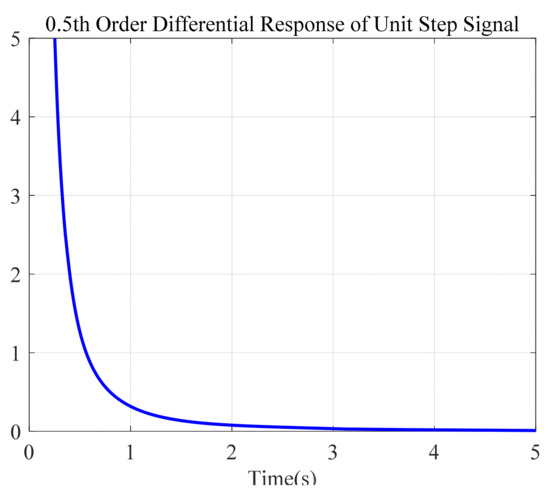
Figure 3. The fractional differential curve of the unit step signal.

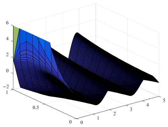
Figure 4. Three-dimensional fractional differential diagram of the sinusoidal function under different orders.

As evident from Figure 3, the 0.5-th-order differential response of the unit step signal does not manifest as a pure impulse. The fractional differential value surges toward infinity at the initial moment, followed by a gradual decline. This behavior underscores the memory capability inherent to fractional-order calculus.

Figure 4 presents a 3D visualization of the fractional differential of a sinusoidal function $y\left(t\right)=\sin \left(3t+1\right)$ across different orders. The fractional derivative alternates between sinusoidal and cosine signals, highlighting the enhanced information captured by fractional calculus.

3.2. Design of Continuous-Time Equal-Order Fractional Butterworth Filter

Given its advantages, the FO calculus is employed to approximate the BW filter response through a novel fractional-order BW (FOBW) filter design. While FO filters offer greater flexibility than IO filters, this flexibility can complicate controller tuning. To address this, an EFBW filter is introduced to reduce the number of tunable parameters and maintain appropriate degrees of freedom. The definition of an equal-order fractional system is provided first.

Lemma 1. [44]

In a fractional differential equation, all fractional orders are integer multiples of a basic order, denoted as $\alpha$ i.e., $\alpha$ is the greatest common divisor) to satisfy ${\alpha }_i,{\beta }_j=k\alpha , \alpha \in {ℝ}^{+}, k\in {ℝ}^{+}$.

Applying Lemma 1 to Equation (18) yields

$$G\left(s\right)={\displaystyle \frac{b_m{s}^{k_m\alpha }+b_{m-1}{s}^{k_{m-1}\alpha }+\dots +b_i{s}^{k_i\alpha }+\dots +b_1{s}^{k_1\alpha }+b_0{s}^{k_0\alpha }}{a_n{s}^{k_n\alpha }+a_{n-1}{s}^{k_{n-1}\alpha }+\dots +a_j{s}^{k_j\alpha }+\dots +a_1{s}^{k_1\alpha }+a_0{s}^{k_0\alpha }}}$$

(19)

Let $\lambda =s^{\alpha }$, then Equation (19) can be rewritten as

$$G\left(\lambda \right)={\displaystyle \frac{{\displaystyle \sum _{i=0}^m{b}_i{\lambda }^{k_i}}}{{\displaystyle \sum _{j=0}^n{a}_j{\lambda }^{p_j}}}}$$

(20)

Once the equal-order fractional system is defined, the general procedure for the EFBW filter is as follows. First, consider a normalized low-pass Butterworth (BW) filter [45], which has the following magnitude equation:

$$H\left(\mathsf{\Omega }\right)={\displaystyle \frac{1}{\sqrt{1+{\mathsf{\Omega }}_n^{2N}}}}$$

(21)

where $N$ is a positive integer representing the filter order, ${\mathsf{\Omega }}_n=\mathsf{\Omega }/{\mathsf{\Omega }}_c$ is the normalized frequency, and ${\mathsf{\Omega }}_c$ is the cutoff frequency

The magnitude squared function of the characteristic polynomial is derived from Equation (21) as

$${\left|D\left(\mathrm{j}\mathsf{\Omega }\right)\right|}^2=1+{\mathsf{\Omega }}_n^{2\mathrm{N}}$$

(22)

To generalize the EFBW filter design beyond the integer-order filter, the above equation is modified by expressing ${\left|D\left(j\mathsf{\Omega }\right)\right|}^2$ as a fractional-order function through the following expression:

$${\left|D\left(\mathrm{j}\mathsf{\Omega }\right)\right|}^2=1+{\mathsf{\Omega }}_n^{2m}$$

(23)

where $m$ is a real positive number.

The general form of the low-pass FO filter transfer function is given by

$$\overline{H}\left(s\right)={\displaystyle \frac{k_1}{s^{\alpha +\beta }+b_1{s}^{\alpha }+b_2{s}^{\beta }+c}}$$

(24)

where the design parameters $b_1,b_2,c,k_1>0$ and $\alpha ,\beta \in \left(0,2\right]$ denote the fractional orders of the filter.

The primary objective is to approximate the transfer function of the FO low-pass filter to that of a BW filter by determining the coefficients. In the case of the equal order, i.e., $\alpha =\beta$, Equation (24) can be written as

$$\overline{H}\left(s\right)={\displaystyle \frac{k_1}{s^{2\alpha }+b{s}^{\alpha }+c}}$$

(25)

where $b=b_1+b_2$. To achieve a normalized pass-band gain, $c$ must be equal to $k_1$ in the transfer function [46]. The following aims at designing the equal-order fractional filter to satisfy the BW response by calculating filter coefficients $b, c, k_1$.

When $\mathrm{s}=\mathrm{j}\mathsf{\Omega }$, the characteristic polynomial of Equation (24) equals to

$$\overline{D}\left(\mathrm{j}\mathsf{\Omega }\right)=\left({\mathsf{\Omega }}^{2\alpha }\cos \left(\alpha \pi \right)+b{\mathsf{\Omega }}^{\alpha }\cos \left({\displaystyle \frac{\alpha \pi }{2}}\right)+c\right)+\mathrm{j}\left({\mathsf{\Omega }}^{2\alpha }\sin \left(\alpha \pi \right)+b{\mathsf{\Omega }}^{\alpha }\sin \left({\displaystyle \frac{\alpha \pi }{2}}\right)\right)$$

(26)

The magnitude squared function of Equation (26) can be deduced as

$${\left|\overline{D}\left(\mathrm{j}\mathsf{\Omega }\right)\right|}^2={\mathsf{\Omega }}^{4\alpha }+2b\left({\mathsf{\Omega }}^{3\alpha }+c{\mathsf{\Omega }}^{\alpha }\right)\cos \left({\displaystyle \frac{\alpha \pi }{2}}\right)+\left(b^2+2c\cos \left(\alpha \pi \right)\right){\mathsf{\Omega }}^{2\alpha }+c^2$$

(27)

To approximate the BW filter response, the magnitude squared function of Equation (27) should be similar to Equation (23) as

$${\left|\overline{D}\left(\mathrm{j}\mathsf{\Omega }\right)\right|}^2=c^2+{\mathsf{\Omega }}^{4\alpha }$$

(28)

By comparing Equation (23) with Equation (28), the cutoff frequency is obtained as

$${\mathsf{\Omega }}_c=c^{{\displaystyle \frac{1}{2\alpha }}}$$

(29)

Therefore, the remaining terms of Equation (27) should be equal to zero, expressed by

$$2b\left({\mathsf{\Omega }}^{3\alpha }+c{\mathsf{\Omega }}^{\alpha }\right)\cos \left({\displaystyle \frac{\alpha \pi }{2}}\right)+\left(b^2+2c\cos \left(\alpha \pi \right)\right){\mathsf{\Omega }}^{2\alpha }=0$$

(30)

Define ${\mathsf{\eta }}^{\alpha }=b{\mathsf{\Omega }}^{\alpha }/\mathrm{c}$ and $\mathsf{\xi }=\mathrm{c}/b^2$, then Equation (30) is equal to

$${\mathsf{\xi }\mathsf{\eta }}^{2\alpha }+\left({\displaystyle \frac{2\xi \cos \left(\alpha \pi \right)+1}{2\cos \left(\frac{\alpha \pi }{2}\right)}}\right){\mathsf{\eta }}^{\alpha }+1=0$$

(31)

The expression between $\mathsf{\eta }$ and $\mathsf{\xi }$ at ${\mathsf{\Omega }}_c$ is given by

$$\mathsf{\xi }={\displaystyle \frac{1}{{\mathsf{\eta }}^{2\alpha }}}$$

(32)

By analyzing the range of $\alpha$, the solution of Equation (31) can be divided into three different cases:

$$\mathsf{\eta }=\left\{\begin{array}{c}0\hspace{1em}\hspace{1em}\hspace{1em}\hspace{1em}\hspace{1em}\hspace{1em}\hspace{1em}\hspace{1em}\hspace{1em}\hspace{1em}0<\alpha <0.5\\ {\left(-2\cos \left(0.5\alpha \pi \right)+\sqrt{2}\right)}^{{\displaystyle \frac{1}{\alpha }}}\hspace{0.33em}\hspace{1em}0.5\le \alpha <1.5\\ {\left(-2\cos \left(0.5\alpha \pi \right)\pm \sqrt{2}\right)}^{{\displaystyle \frac{1}{\alpha }}}\hspace{0.33em}\hspace{1em}1.5\le \alpha <2.0\end{array}\right.$$

(33)

Consequently, once the fractional order $\alpha$ is known, $\mathsf{\eta }$ can be calculated using Equation (33). Subsequently, the filter coefficients $b, c, k_1$ can be determined for the fixed cutoff frequency ${\mathsf{\Omega }}_c$. This process enables the realization of the continuous-time EFBW filter.

3.3. Design Advantages of EFBW Filter

From Equations (24), (25), and (31), it is obtained that the two variables $b_1, b_2$ are consolidated into a single parameter $b$ as $b=b_1+b_2$. This reduces the degrees of freedom of the EFBW filter compared to different-order fractional BW filters $\alpha \ne \beta$. Therefore, the proposed EFBW filter reduces tunable parameters to achieve appropriate degrees of freedom. Figure 5 presents a frequency characteristics diagram of the BW filters across different orders. The magnitude characteristics diagram shows that the 2.2-th- to 2.8-th-order FOBW filters approximate the ideal response better than the 2nd-order filter. Meanwhile, the phase characteristics diagram indicates that the 2.2-th- to 2.8-th-order FOBW filters have less phase lag than the 3rd-order filter. Therefore, compared to the IOBW filter, the EFBW filter demonstrates an improved balance between magnitude response and phase characteristics.

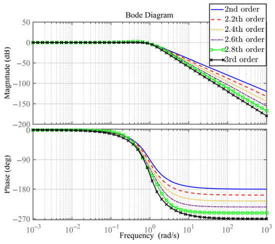
Figure 5. The frequency characteristics of the BW filter in different orders.

It is important to mention that the ideal BW filter is not physically realizable, mainly due to the abrupt changes in its frequency response between different frequency bands. Therefore, to achieve physical realizability, four key technical specifications must be addressed: pass-band edge frequency ${\mathsf{\Omega }}_p$, stop-band edge frequency ${\mathsf{\Omega }}_{\mathrm{s}}$, maximum pass-band attenuation $A_p$, and minimum stop-band attenuation $A_{\mathrm{s}}$ [47]. By optimizing these parameters, the optimal order $N$ and cutoff frequency ${\mathsf{\Omega }}_c$ of the low-pass BW filter can easily be obtained as

$$N=\lg \sqrt{{\displaystyle \frac{{10}^{A_{\mathrm{s}}/10}-1}{{10}^{A_p/10}-1}}}/\lg {\displaystyle \frac{{\mathsf{\Omega }}_{\mathrm{s}}}{{\mathsf{\Omega }}_p}}$$

(34)

$${\mathsf{\Omega }}_c={{\mathsf{\Omega }}_{\mathrm{s}}/\left({10}^{A_{\mathrm{s}}/10}-1\right)}^{1/2N}$$

(35)

Obviously, the optimal order $N$ may be an integer or a fraction. For IOBW filters, the optimal fractional orders are typically rounded to the nearest integer due to the lack of FO options, which introduces some approximation error. In contrast, the EFBW filter can precisely meet technical specifications without under- or oversatisfying design requirements.

3.4. Discretization Algorithm

In this section, the design of the EFBW filter for discrete-time applications is addressed. An efficient approximation algorithm based on impulse response is employed, aiming to derive a rational discrete-time transfer function for the EFBW filter from its continuous-time counterpart.

The first step is to discretize the equal fractional-order Laplace operator $s^{\alpha }$ using appropriate generating functions, which are expressed as follows.

• Euler transformation:

$$s\left(z^{-1}\right)={\displaystyle \frac{1-z^{-1}}{T}}$$

• Tustin transformation:

$$s\left(z^{-1}\right)={\displaystyle \frac{2}{T}}\left({\displaystyle \frac{1-z^{-1}}{1+z^{-1}}}\right)$$

where $z=e^{sT}$ is the ordinary $z$ transformation, and $T$ is the sample time. The above classical transformations, which map the Laplace operator $s$ to the discrete-time operator $z^{-1}$, can provide a good discrete-time approximation for a continuous-time transfer function if $T$ is selected appropriately. To construct the generating function, an interpolation of the Euler and Tustin discretization transformations is used, expressed as

$$s\left(z^{-1}\right)={\displaystyle \frac{\left(1+\rho \right)\left(1-z^{-1}\right)}{T\left(1+\rho z^{-1}\right)}}$$

(36)

where $\rho \in \left[0, 1\right]$ is a weight that balances the interpolation between the Euler and Tustin transformations. Note that $\rho =0$ leads to the Euler transformation, while $\rho =1$ corresponds to the Tustin transformation.

The main objective in this step is to create a discrete-time operator ${\left(s\left(z^{-1}\right)\right)}^{\alpha }$ for the EFBW filter, replacing $s^{\alpha }$ via Equation (36) within the proper frequency range $\mathsf{\Omega }\in \left(0, {\mathsf{\Omega }}_{\mathrm{h}}\right)$, given a specific weight $\rho$ and maximum frequency ${\mathsf{\Omega }}_{\mathrm{h}}$. According to the Nyquist sampling theorem [47], the maximum sampling period is selected as $T=\pi /{\mathsf{\Omega }}_{\mathrm{h}}$.

The frequency response is utilized as the basis for computing the impulse response, aiming to avoid the computational complexity that would otherwise be caused by the impulse response of the discrete-time EFBW filter. Based on $z^{-1}=e^{-sT}$, the operator $z^{-1}$ should be replaced with $z^{-1}=e^{-j\mathsf{\Omega }T}$ to obtain the frequency response of the discrete-time EFBW filter $\overline{H}\left(e^{-j\mathsf{\Omega }T}\right)$, where $\mathsf{\Omega }={\displaystyle \frac{2\pi }{L_{s}T}}\left[0\hspace{1em}1\hspace{1em}2\hspace{1em}{\displaystyle \frac{L_s}{2}}\right]$ is a vector of equally spaced frequencies, $L_s$ is the total number of samples. The bigger the value of $L_s$, the better the approximation performance. Furthermore, the inverse Fast Fourier Transform (FFT) algorithm is used to transform the frequency response of the discrete-time EFBW filter into an impulse response at discrete intervals $\left[0, T, 2T, \dots , \left(L_s-1\right)T\right]$.

The impulse response is given by

$$\overline{h}\left(n\right)={\displaystyle \frac{1}{L_s}}{\displaystyle \sum _{k=0}^{L_s-1}\overline{H}\left[k\right]e^{+j\frac{2\pi }{L_{s}nk}}}, n=0, 1, \dots , L_s-1$$

(37)

where $\overline{H}\left[k\right]$ is the frequency response of $\overline{H}\left(s\right)$.

Finally, the discrete-time transfer function of the EFBW filter is determined to match the impulse response derived from the inverse FFT, resulting in a complexity of O(N log N), described by

$$\overline{H}\left(z^{-1}\right)={\displaystyle \frac{e_0+e_1{z}^{-1}+\dots +e_N{z}^{-L}}{f_0+f_1{z}^{-1}+\dots f_N{z}^{-L}}}$$

(38)

in which the discrete-time transfer function of the EFBW filter is obtained using the simple signal modeling technique described in [48], with its coefficients $e_i, f_i, \left(i=1, 2, \dots , L\right)$ determined by the desired order $L$.

4. Stability Analysis

Theorem 1 [2] (Internal Stability).

If the plant $P\left(z\right)$ is stable and the discrete-time model $P_{\mathrm{m}}\left(z\right)$ perfectly describes the plant $P\left(z\right)$, then the stability of the controller $C\left(z\right)$ is equivalent to the internal stability of the overall system.

According to Equations (13) and (14), the stability of the controller $C\left(\mathrm{s}\right)$ is characterized by the stability of the EFBW filter. In a discrete-time ID-IMC system, the internal stability is guaranteed as long as the poles of $\overline{H}\left(z\right)$ lie inside the unit circle. Once the internal stability is achieved, the ID-IMC framework enables designers to concentrate solely on optimizing system performance and robustness.

5. Robustness Analysis

The model mismatch in MIMO systems is highly intricate, and cannot be merely dissected into individual SISO cases due to the coupling in $P\left(z\right)$ is coupled. Therefore, the robustness analysis for the model mismatch of $P\left(z\right)$ using the structured singular value (SSV) $\mu -$ analysis is carried out to evaluate the robust stability (RS) and robust performance (RP) of the proposed discrete-time ID-IMC controller. Similarly to the continuous-time case, multiplicative input uncertainty $\mathsf{\Delta }$ is added, where the diagonal matrices $W_I$ and $W_P$ represent the uncertainty weight function and the performance weight function, as shown in Figure 6.

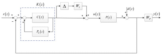
Figure 6. The discrete-time ID-IMC system with multiplicative input uncertainty.

To achieve RS and RP, the following necessary and sufficient conditions must be met [49]:

$${\mu }_{\mathrm{RS}}\iff \mu \left[W_I{T}_I\left(z\right)\right]<1, \forall \omega >0$$

(39)

$${\mu }_{\mathrm{RP}}\iff \mu \left[\begin{array}{cc}-W_I{T}_I\left(z\right)& -W_{I}K\left(z\right)S_I\left(z\right)\\ W_P{S}_I\left(z\right)P\left(z\right)& W_P{S}_I\left(z\right)\end{array}\right]<1, \forall \omega >0$$

(40)

where $K\left(z\right)=C\left(z\right){\left(I-P_m\left(z\right)C\left(z\right)\right)}^{-1}$, $S_I\left(z\right)={\left(I+P\left(z\right)K\left(z\right)\right)}^{-1}$ is the sensitivity transfer matrix, and $T_I\left(z\right)=K\left(z\right)P\left(z\right){\left(I+K\left(z\right)P\left(z\right)\right)}^{-1}$ is the complementary sensitivity transfer matrix.

6. Simulations

To illustrate the proposed controller design method, simulation results are carried out on two typical IO processes.

Example 1.

Consider the two-input-two-output (TITO) binary distillation column model [50] as follows:

$$P\left(\mathrm{s}\right)=\left[\begin{array}{cc}{\overline{p}}_{11}\left(s\right)& {\overline{p}}_{12}\left(s\right)\\ {\overline{p}}_{21}\left(s\right)& {\overline{p}}_{22}\left(s\right)\end{array}\right]=\left[\begin{array}{cc}{\displaystyle \frac{12.8e^{-s}}{16.7s+1}}& {\displaystyle \frac{-18.9e^{-3s}}{21s+1}}\\ {\displaystyle \frac{6.6e^{-7s}}{10.9s+1}}& {\displaystyle \frac{-19.4e^{-3s}}{14.4s+1}}\end{array}\right]$$

(41)

The sampling time is set to $T=0.5\mathrm{s}$; thereby, the discrete-time model of the process is given by

$$\begin{array}{l}P\left(z\right)=\left[\begin{array}{cc}{\overline{p}}_{11}\left(z\right)& {\overline{p}}_{12}\left(z\right)\\ {\overline{p}}_{21}\left(z\right)& {\overline{p}}_{22}\left(z\right)\end{array}\right]\\ =\left[\begin{array}{cc}{z}^{-2}{\displaystyle \frac{0.3776}{z-0.9705}}& z^{-6}{\displaystyle \frac{0.4447}{z-0.9917}}\\ z^{-14}{\displaystyle \frac{0.2959}{z-0.9552}}& z^{-6}{\displaystyle \frac{-0.6621}{z-0.9659}}\end{array}\right]\end{array}$$

(42)

The technical specifications of the EFBW are given as $A_p=4 \mathrm{dB}$, $A_s=12 \mathrm{dB}$, ${\mathsf{\Omega }}_p=2 \mathrm{rad}/\mathrm{s}$, and ${\mathsf{\Omega }}_s= 4.5\mathrm{rad}/\mathrm{s}$, then according to Equations (34) and (35), the optimal order $N$ and cutoff frequency ${\mathsf{\Omega }}_c$ are calculated as $N=1.4$ and ${\mathsf{\Omega }}_c=1.73 \mathrm{rad}/\mathrm{s}$. By Equations (25) and (29), the continuous-time EFBW filter is obtained as

$$\overline{H}\left(\mathrm{s}\right)={\displaystyle \frac{4.55}{s^{1.4}+5.53s^{0.7}+4.55}}$$

(43)

Using the discretization algorithm proposed in Equation (38), with $L=4$, $\rho =0.9$, $T=0.5 \mathrm{s}$, the discrete-time transfer function of the continuous-time EFBW filter is given by

$$\overline{H}\left(z^{-1}\right)={\displaystyle \frac{{0.1812z}^0+0.02999z^{-1}-0.2389z^{-2}-0.0266z^{-3}+0.06964z^{-4}}{z^0-1.266z^{-1}-0.2216z^{-2}+0.6506z^{-3}-0.1468z^{-4}}}$$

(44)

The frequency responses for the continuous-time and discrete-time EFBW filters are shown in Figure 7, which suggests that the proposed discrete-time filter can approximate the frequency response of the original continuous-time EFBW filter. Figure 8 shows that all the poles are distributed in the unit circle, which means that the EFBW filter is stable, and the closed-loop system is stable according to Theorem 1.

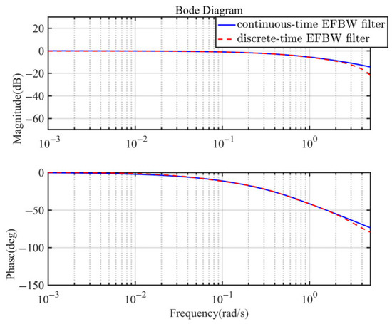
Figure 7. Frequency responses for the continuous-time and discrete-time EFBW filters.

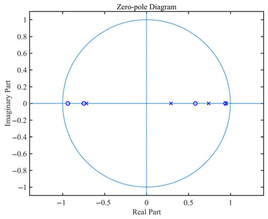
Figure 8. The zero-pole map of the discrete-time EFBW filter.

From Equation (42), the minimum time-delay terms in each row of the process model transfer matrix are ${\overline{p}}_{11}\left(z\right)$ and ${\overline{p}}_{22}\left(z\right)$. According to Equations (6) and (7), the elements $c_{{\mathrm{d}}_{11}}\left(z\right)$ and $c_{{\mathrm{d}}_{22}}\left(z\right)$ are chosen to be non-zero. In order to meet the realizable conditions by Equations (9) and (10), the time-delay terms of the desired closed-loop transfer functions $t_1\left(z\right)$ and $t_2\left(z\right)$ are chosen to be ${\tau }_1=2$ and ${\tau }_2=6$, respectively. Then applying Equation (37) to Equation (43), the desired system closed-loop transfer matrix $T\left(z\right)=\mathrm{diag}\left(t_1\left(z\right), t_2\left(z\right)\right)$ is calculated as

$$\begin{array}{l}{t}_1\left(z\right)=z^{-{\tau }_1}{\displaystyle \prod _{x=1}^N}{\left[{\displaystyle \frac{z-{\sigma }_x}{z-{\widehat{\sigma }}_x}}\right]}^{{\upsilon }_i}\overline{H}\left(z\right)\\ \hspace{1em}\hspace{1em}=z^{-2}{\displaystyle \frac{{0.1812z}^0+0.02999z^{-1}-0.2389z^{-2}-0.0266z^{-3}+0.06964z^{-4}}{z^0-1.266z^{-1}-0.2216z^{-2}+0.6506z^{-3}-0.1468z^{-4}}}\end{array}$$

(45)

$$\begin{array}{l}{t}_2\left(z\right)=z^{-{\tau }_2}{\displaystyle \prod _{x=1}^N}{\left[{\displaystyle \frac{z-{\sigma }_x}{z-{\widehat{\sigma }}_x}}\right]}^{{\upsilon }_i}\overline{H}\left(z\right)\\ \hspace{1em}\hspace{1em}=z^{-6}{\displaystyle \frac{{0.1812z}^0+0.02999z^{-1}-0.2389z^{-2}-0.0266z^{-3}+0.06964z^{-4}}{z^0-1.266z^{-1}-0.2216z^{-2}+0.6506z^{-3}-0.1468z^{-4}}}\end{array}$$

(46)

Substituting Equations (42), (45), and (46) into Equations (13) and (14) yields

$$c_{{\mathrm{d}}_{11}}\left(z\right)={\displaystyle \frac{t_1\left(z\right)}{p_{11}\left(z\right)}}={\displaystyle \frac{\left(z-0.6894\right)\left({0.1812z}^0+0.02999z^{-1}-0.2389z^{-2}-0.0266z^{-3}+0.06964z^{-4}\right)}{0.3776\left(z-0.5\right)\left(z^0-1.266z^{-1}-0.2216z^{-2}+0.6506z^{-3}-0.1468z^{-4}\right)}}$$

(47)

$$c_{{\mathrm{d}}_{22}}\left(z\right)={\displaystyle \frac{t_2\left(z\right)}{p_{22}\left(z\right)}}=-{\displaystyle \frac{\left(z-0.9659\right)\left({0.1812z}^0+0.02999z^{-1}-0.2389z^{-2}-0.0266z^{-3}+0.06964z^{-4}\right)}{0.6621\left(z-0.5\right)\left(z^0-1.266z^{-1}-0.2216z^{-2}+0.6506z^{-3}-0.1468z^{-4}\right)}}$$

(48)

$$c_{{\mathrm{o}}_{12}}\left(s\right)=-{\displaystyle \frac{p_{12}\left(z\right)}{t_1\left(z\right)}}=z^{-4}{\displaystyle \frac{0.4447\left(z-0.5\right)\left(z^0-1.266z^{-1}-0.2216z^{-2}+0.6506z^{-3}-0.1468z^{-4}\right)}{\left(z-0.9765\right)\left({0.1812z}^0+0.02999z^{-1}-0.2389z^{-2}-0.0266z^{-3}+0.06964z^{-4}\right)}}$$

(49)

$$c_{{\mathrm{o}}_{21}}\left(z\right)=-{\displaystyle \frac{p_{21}\left(z\right)}{t_2\left(z\right)}}=-z^{-8}{\displaystyle \frac{0.2959\left(z-0.5\right)\left(z^0-1.266z^{-1}-0.2216z^{-2}+0.6506z^{-3}-0.1468z^{-4}\right)}{\left(z-0.9552\right)\left({0.1812z}^0+0.02999z^{-1}-0.2389z^{-2}-0.0266z^{-3}+0.06964z^{-4}\right)}}$$

(50)

where the diagonal matrix $D\left(z\right)$ is introduced as the multiplicative factor of $P\left(z\right)$ in Equation (42), to satisfy the physical realizability of the system

$$D\left(z\right)=\left[\begin{array}{cc}z-0.5& 0\\ 0& z-0.5\end{array}\right]$$

(51)

Figure 9 and Figure 10 illustrate the system output and controller output responses of the proposed method. Unit step changes are added into the two input variables of the model, as the step changes of 0.2 magnitude are added at $t=50\mathrm{s}$. Figure 9 indicates that the proposed method’s output variables track the unit step signal more quickly than the conventional low-pass filter method. They also recover faster from disturbances, highlighting the proposed method’s superior anti-disturbance capability. Figure 10 reveals that the controller output curves using the EFBW filter are smoother, with less chattering and a better decoupling effect.

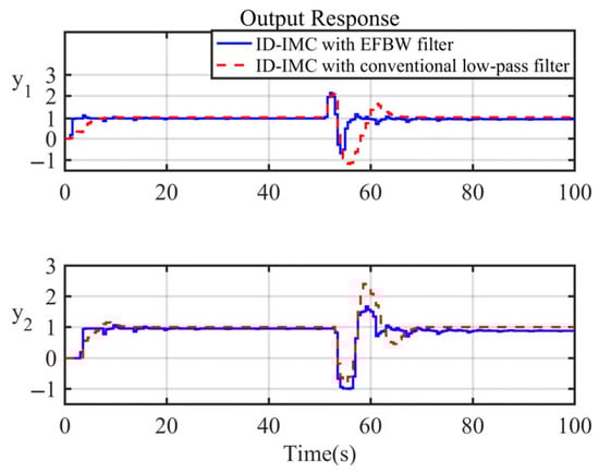
Figure 9. The system output response.

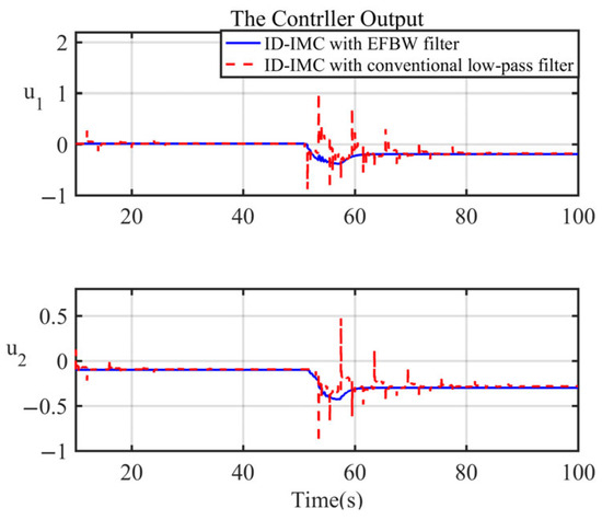
Figure 10. The controller output.

For robustness analysis, structured singular values for the RS and RP are shown in Figure 11, where the uncertainty weight function is chosen as $W_I=\left(s+0.2\right)\cdot I/\left(s+1\right)$, representing approximately 20% uncertainties in the low frequencies and 100% uncertainties in the high frequencies. The performance weight function is given by $W_P=\left(s/2.2+0.001\right)\cdot I/s$, where the maximum peak for the singular value of the sensitivity transfer matrix is selected as 2.2 and the bandwidth is 0.001 rad/s. It can be seen that the proposed method remains robust stable and has good robust performance since the RS and RP are less than 1 in all frequencies.

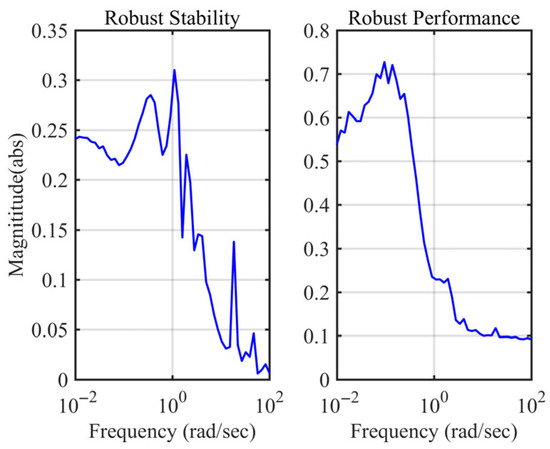
Figure 11. The robust stability and robust performance of Example 1.

Example 2.

The continuous-time plant is given by Equation (52). It has time-delays and multivariable NMP zeros at $s=1$.

$$P\left(s\right)=\left[\begin{array}{cc}{\overline{p}}_{11}\left(s\right)& {\overline{p}}_{12}\left(s\right)\\ {\overline{p}}_{21}\left(s\right)& {\overline{p}}_{22}\left(s\right)\end{array}\right]=\left[\begin{array}{cc}{\displaystyle \frac{\left(-s+1\right)e^{-s}}{15.1\mathrm{s}+1}}& -{\displaystyle \frac{\left(-s+1\right)e^{-3s}}{15.1s+1}}\\ {\displaystyle \frac{4.4e^{-7s}}{13.6s+1}}& -{\displaystyle \frac{6.3e^{-3s}}{14.2s+1}}\end{array}\right]$$

(52)

For a sampling time $T=0.5\mathrm{s}$, the corresponding discrete-time transfer matrix is given by

$$P\left(z\right)=\left[\begin{array}{cc}{\overline{p}}_{11}\left(z\right)& {\overline{p}}_{12}\left(z\right)\\ {\overline{p}}_{21}\left(z\right)& {\overline{p}}_{22}\left(z\right)\end{array}\right]=\left[\begin{array}{cc}{z}^{-2}{\displaystyle \frac{-0.06623z+0.0988}{z-0.9674}}& z^{-6}{\displaystyle \frac{0.06623z-0.0988}{z-0.9674}}\\ z^{-14}{\displaystyle \frac{0.1588}{z-0.9638}}& z^{-6}{\displaystyle \frac{-0.218}{z-0.9654}}\end{array}\right]$$

(53)

Similar to Example 1, $c_{{\mathrm{d}}_{11}}\left(z\right)$ and $c_{{\mathrm{d}}_{22}}\left(z\right)$ are selected to be non-zero. Due to the realizable conditions given by Equations (9) and (10), the minimum time-delays in Loop 1 and Loop 2 are chosen to be ${\tau }_1=2$ and ${\tau }_2=6$, respectively. The smallest zero multiplicity outside the unit circle in Loop 1 is 1.49. Hence, according to Equation (11) and the discrete-time EFBW filter given by Equation (44), the desired closed-loop transfer matrix $T\left(z\right)=\mathrm{diag}\left(t_1\left(z\right),t_2\left(z\right)\right)$ is obtained as

$$\begin{array}{l}{t}_1\left(z\right)=z^{-{\tau }_1}{\displaystyle \prod _{x=1}^N}{\left[{\displaystyle \frac{z-{\sigma }_x}{z-{\widehat{\sigma }}_x}}\right]}^{{\upsilon }_i}\overline{H}\left(z\right)\\ \hspace{1em}\hspace{1em}=z^{-2}{\displaystyle \frac{\left(z-1.49\right)\left({0.1812z}^0+0.02999z^{-1}-0.2389z^{-2}-0.0266z^{-3}+0.06964z^{-4}\right)}{\left(z-0.67\right)\left(z^0-1.266z^{-1}-0.2216z^{-2}+0.6506z^{-3}-0.1468z^{-4}\right)}}\end{array}$$

(54)

$$\begin{array}{l}{t}_2\left(z\right)=z^{-{\tau }_2}{\displaystyle \prod _{x=1}^N}{\left[{\displaystyle \frac{z-{\sigma }_x}{z-{\widehat{\sigma }}_x}}\right]}^{{\upsilon }_i}\overline{H}\left(z\right)\\ \hspace{1em}\hspace{1em}=z^{-6}{\displaystyle \frac{{0.1812z}^0+0.02999z^{-1}-0.2389z^{-2}-0.0266z^{-3}+0.06964z^{-4}}{z^0-1.266z^{-1}-0.2216z^{-2}+0.6506z^{-3}-0.1468z^{-4}}}\end{array}$$

(55)

By means of Equations (13) and (14), the forward channel transfer matrix $C_{\mathrm{d}}\left(z\right)$ and the feedback channel transfer matrix $C_{\mathrm{o}}\left(z\right)$ are obtained as

$$c_{{\mathrm{d}}_{11}}\left(s\right)={\displaystyle \frac{t_1\left(s\right)}{p_{11}\left(s\right)}}=-{\displaystyle \frac{\left(z-0.9674\right)\left({0.1812z}^0+0.02999z^{-1}-0.2389z^{-2}-0.0266z^{-3}+0.06964z^{-4}\right)}{0.06623\left(z-0.67\right)\left(z^0-1.266z^{-1}-0.2216z^{-2}+0.6506z^{-3}-0.1468z^{-4}\right)}}$$

(56)

$$c_{{\mathrm{d}}_{22}}\left(s\right)={\displaystyle \frac{t_2\left(s\right)}{p_{22}\left(s\right)}}=-{\displaystyle \frac{\left(z-0.9654\right)\left({0.1812z}^0+0.02999z^{-1}-0.2389z^{-2}-0.0266z^{-3}+0.06964z^{-4}\right)}{0.218\left(z-0.5\right)\left(z^0-1.266z^{-1}-0.2216z^{-2}+0.6506z^{-3}-0.1468z^{-4}\right)}}$$

(57)

$$c_{{\mathrm{o}}_{12}}\left(s\right)=-{\displaystyle \frac{p_{12}\left(s\right)}{t_1\left(s\right)}}=-z^{-4}{\displaystyle \frac{0.06623\left(z-0.67\right)\left(z^0-1.266z^{-1}-0.2216z^{-2}+0.6506z^{-3}-0.1468z^{-4}\right)}{\left(z-0.9674\right)\left({0.1812z}^0+0.02999z^{-1}-0.2389z^{-2}-0.0266z^{-3}+0.06964z^{-4}\right)}}$$

(58)

$$c_{{\mathrm{o}}_{21}}\left(s\right)=-{\displaystyle \frac{p_{21}\left(s\right)}{t_2\left(s\right)}}=-z^{-8}{\displaystyle \frac{0.1588\left(z^0-1.266z^{-1}-0.2216z^{-2}+0.6506z^{-3}-0.1468z^{-4}\right)}{\left(z-0.9638\right)\left({0.1812z}^0+0.02999z^{-1}-0.2389z^{-2}-0.0266z^{-3}+0.06964z^{-4}\right)}}$$

(59)

The system output response curves are shown in Figure 12, where Figure 12a shows the unit step changes applied to the process inputs, while Figure 12b illustrates the addition of 0.2 magnitude step disturbances at $t=150\mathrm{s}$. It can be observed that the proposed method using the EFBW filter exhibits less overshoot and superior disturbance rejection compared to the conventional low-pass filter method. Figure 13a,b indicate that the proposed method yields smoother controller output curves with better decoupling performance, even when subjected to disturbances.

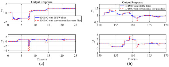
Figure 12. (a) The system output response of (0–25 s); (b) the system output response of (150–170 s).

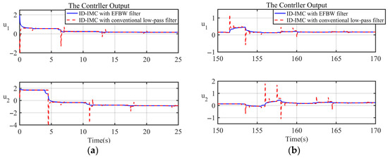
Figure 13. (a) The controller output of (0–25 s); (b) the controller output of (150–170 s).

Similar to Example 1, choosing $W_I=\left(s+0.1\right)\cdot I/\left(s+1\right)$ and $W_P=\left(s/2.5+0.001\right)\cdot I/s$, the $\mu -$ analysis process is applied to evaluate the RS and RP. As shown in Figure 14, the proposed method is robust stable in all frequencies, as the peak value of the RS and RP curves is less than 1.

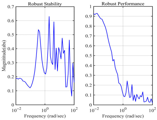
Figure 14. The robust stability and robust performance of Example 2.

7. Conclusions

A novel discrete-time ID-IMC controller based on a discrete-time EFBW filter has been proposed for multivariable systems with time-delays and non-minimum zeros in this paper. The proposed strategy makes use of the discrete-time EFBW filter to obtain a good trade-off between the additional flexibility and the design complexity. By combining the discrete-time EFBW filter with the discrete-time ID-IMC controller, we obtain a desired set-point tracking and decoupling effect with provable guarantees of stability and robustness. Two simulation examples show that the proposed method has a better performance in the set-point tracking and robustness compared with the conventional IMC method.

References

- Garcia, C.E.; Morari, M. Internal model control. A unifying review and some new results. Ind. Eng. Chem. Process Des. Dev. 1982, 21, 308–323. [Google Scholar] [CrossRef]
- Garcia, C.E.; Morari, M. Internal model control. 2. Design procedure for multivariable systems. Ind. Eng. Chem. Process Des. Dev. 1985, 24, 472–484. [Google Scholar] [CrossRef]
- Ouardani, D.; Bodian, A.; Cardenas, A. Comparative Analysis of PID and Robust IMC Control in Cascaded Processes with Time-Delay. IEEE Access 2024, 12, 14199–142014. [Google Scholar] [CrossRef]
- Xie, J.; Bonassi, F.; Scattolini, R. Learning Control Affine Neural NARX Models for Internal Model Control Design. IEEE Trans. Autom. Sci. Eng. 2025, 22, 8137–8149. [Google Scholar] [CrossRef]
- Maamar, B.; Rachid, M. IMC-PID-fractional-order-filter controllers design for integer order systems. ISA Trans. 2014, 53, 1620–1628. [Google Scholar] [CrossRef]
- Bettayeb, M.; Mansouri, R. Fractional IMC-PID-filter controllers design for non integer order systems. J. Process Control 2014, 24, 261–271. [Google Scholar] [CrossRef]
- Li, D.; Liu, L.; Jin, Q.; Hirasawa, K. Maximum sensitivity based fractional IMC–PID controller design for non-integer order system with time delay. J. Process Control 2015, 31, 17–29. [Google Scholar] [CrossRef]
- Cui, J.; Chen, Y.; Liu, T. Discrete-time domain IMC-based PID control design for industrial processes with time delay. In Proceedings of the 2016 35th Chinese Control Conference (CCC), Chengdu, China, 27–29 July 2016; IEEE: New York, NY, USA; pp. 5946–5951. [Google Scholar]
- De Keyser, R.; Copot, C.; Hernandez, A.; Ionescu, C. Discrete-time internal model control with disturbance and vibration rejection. J. Vib. Control 2017, 23, 3–15. [Google Scholar] [CrossRef]
- Silva, G.J.; Datta, A. Adaptive internal model control: The discrete-time case. Int. J. Adapt. Control Signal Process. 2001, 15, 15–36. [Google Scholar] [CrossRef]
- Hannachi, M.; Soudani, D. Internal model control of multivariable discrete-time systems. In Proceedings of the 2015 7th International Conference on Modelling, Identification and Control (ICMIC), Sousse, Tunisia, 18–20 December 2015; IEEE: New York, NY, USA; pp. 1–6. [Google Scholar]
- Touati, N.; Saidi, I. Dahlin Deadbeat Internal Model Control for Discrete MIMO Systems. Int. J. Electr. Comput. Eng. Syst. 2024, 15, 483–490. [Google Scholar] [CrossRef]
- Mondal, R.; Dey, J. On Non-Integer Order Internal Model Control of Non-Minimum Phase Systems and Plants with Transport Delay. In Proceedings of the 2024 IEEE 3rd International Conference on Control, Instrumentation, Energy & Communication (CIEC), Kolkata, India, 25–27 January 2024; IEEE: New York, NY, USA; pp. 37–42. [Google Scholar]
- Ogunba, K.S.; Fakunle, A.A.; Ogunfunmi, T.; Taiwo, O. Extended Approach to Analytical Triangular Decoupling Internal Model Control of Square Stable Multivariable Systems with Delays and Right-Half-Plane Zeros. IEEE Access 2023, 11, 32201–32228. [Google Scholar] [CrossRef]
- Kumar, A.; Anwar, M.N.; Huba, M. Load Frequency Controller Design Based on the Direct Synthesis Approach Using a 2DoF-IMC Scheme for a Multi-Area Power System. Symmetry 2022, 14, 1994. [Google Scholar] [CrossRef]
- Kumar, K.; Patwardhan, S.C.; Noronha, S. Development of an adaptive and explicit dual model predictive controller based on generalized orthogonal basis filters. J. Process Control 2019, 83, 196–214. [Google Scholar] [CrossRef]
- Hasan, M.J.; Bashar, N.; Sarker, S.; Lopa, S.A.; Hamim, T. Harmonic reduction of second order sallen and key lowpass filter and second order MFB lowpass filter through closed loop PID controlled method. Int. J. Inf. Technol. 2024, 16, 2635–2645. [Google Scholar] [CrossRef]
- Speakman, J.; Papasavvas, A.; Francois, G. A robust modifier adaptation method via Hessian augmentation using model uncertainties. J. Process Control 2021, 99, 28–40. [Google Scholar] [CrossRef]
- Gnaneshwar, K.; Trivedi, R.; Sharma, S.; Padhy, P.K. A frequency domain fractional order tilted integral derivative controller design for fractional order time delay processes. Asian J. Control 2025, 27, 1384–1404. [Google Scholar]
- Zhou, Y.; Sun, H.; Xu, J.; Rui, X.; Li, J.; Shi, Y.; Qian, Y. Multisim-based Optimized Design of Butterworth Low-pass Filters. In Proceedings of the 2024 7th International Conference on Electronics, Communications, and Control Engineering (ICECC), Kuala Lumpur, Malaysia, 22–24 March 2024; IEEE: New York, NY, USA; pp. 33–40. [Google Scholar]
- Dahake, V.R.; Patil, M.D.; Vyawahare, V.A. Analysis of networked control system with integer-order and fractional-order PID controllers. Int. J. Control Autom. Syst. 2024, 22, 373–386. [Google Scholar] [CrossRef]
- Joshi, M.; Bhosale, S.R.; Vyawahare, V.A. Fractional-order artificial neural network models for linear systems. Int. J. Dyn. Control 2025, 13, 118. [Google Scholar] [CrossRef]
- Maurya, P.; Paul, N.; Prasad, D.; Singh, R.S. Modified Fractional-Order PID Controller Design for the Mixing Tank Process. Chem. Eng. Technol. 2025, 48, e70026. [Google Scholar] [CrossRef]
- Medjili, F.; Bouguerra, A.; Ladjal, M.; Babes, B.; Ali, E.; Ghoneim, S.S.; Aeggegn, D.B.; Sharaf, A.B.A. HIL co-simulation of an optimal hybrid fractional-order type-2 fuzzy PID regulator based on dSPACE for quadruple tank system. Sci. Rep. 2025, 15, 7583. [Google Scholar] [CrossRef]
- Gnaneshwar, K.; Padhy, P.K. A TDF Fractional Order Controller Design for Time Delay Systems Using IMC Approach. In Proceedings of the 2023 Ninth Indian Control Conference (ICC), Visakhapatnam, India, 18–20 December 2023; IEEE: New York, NY, USA; pp. 425–430. [Google Scholar]
- Znidi, A.; Nouri, A.S. Discrete adaptive sliding mode control for uncertain fractional-order Hammerstein system. Trans. Inst. Meas. Control 2025. [Google Scholar] [CrossRef]
- Morari, M.; Zafiriou, E. Robust Process Control; Prentice Hall: Englewood Cliffs, NJ, USA, 1989. [Google Scholar]
- Acharya, A.; Das, S.; Pan, I.; Das, S. Extending the concept of analog Butterworth filter for fractional order systems. Signal Process. 2014, 94, 409–420. [Google Scholar] [CrossRef]
- Liu, K.; Chen, J. Internal Model Control with Improved Butterworth Filter Based on Inverted Decoupling for Multivariable Systems. In Proceedings of the 2019 IEEE International Conference on Systems, Man and Cybernetics (SMC), Bari, Italy, 6–9 October 2019; pp. 511–517. [Google Scholar]
- De Keyser, R.; Muresan, C.I.; Ionescu, C.M. An efficient algorithm for low-order direct discrete-time implementation of fractional order transfer functions. ISA Trans. 2018, 74, 229–238. [Google Scholar] [CrossRef] [PubMed]
- Aouiche, E.M.; Liu, X.; Aouiche, A.; Hassan, M.A.; Aguida, M.E.; Khan, J.A.; Cao, Y. Dynamic Decoupled Current Control 674 for Smooth Torque of the Open-Winding Variable Flux Reluctance Motor Using Integrated Torque Harmonic Extended State Observer. Processes 2025, 13, 263. [Google Scholar] [CrossRef]
- Wang, L.; Zhang, X.; Han, X.; Ren, Y.; Zhang, B.; Wang, P. A Transformerless Converter with Common-Mode Decoupling in Low-Voltage Hybrid Grids. Processes 2024, 12, 507. [Google Scholar] [CrossRef]
- Zhang, Y.; Zhang, Y. Dual-band dual-polarized antenna using a simple radiation restoration and decoupling structure. IEEE Antennas Wirel. Propag. Lett. 2023, 22, 709–713. [Google Scholar] [CrossRef]
- Tran, D.N.V.; Tran, H.H.; Park, H.C.; Nguyen-Trong, N. Simple Decoupling Structure for Dual-Sense CP MIMO Antenna. In Proceedings of the 2022 International Conference on Advanced Technologies for Communications (ATC), Hanoi Capital, Vietnam, 20–22 October 2022; IEEE: New York, NY, USA; pp. 35–38. [Google Scholar]
- Fu, B.; You, B.; Hu, G. Layered Composite Decoupling Control Based on Regional Dynamic Sparrow Search Algorithm. Processes 2023, 11, 3350. [Google Scholar] [CrossRef]
- Lara, M.; Ruz, M.L.; Mulders, S.P.; Vázquez, F.; Garrido, J. Individual pitch controller with static inverted decoupling for periodic blade load reduction on monopile offshore wind turbines. Ocean Eng. 2025, 334, 121608. [Google Scholar] [CrossRef]
- Huairong, C.; Xi, W.; Haonan, W.; Nannan, G.; Meiyin, Z.; Shubo, Y. Inverted decoupling and LMI-based controller design for a turboprop engine with actuator dynamics. Chin. J. Aeronaut. 2020, 33, 1774–1787. [Google Scholar]
- Shen, L.; Chen, Z.; He, J. Multi-zone integrated iterative-decoupling control of temperature ffeld of large-scale vertical quenching furnaces based on ESRNN. Processes 2023, 11, 2106. [Google Scholar] [CrossRef]
- Song, M.; Liu, H.; Xu, Y.; Wang, D.; Huang, Y. Decoupling adaptive smith prediction model of ffatness closed-loop control and its application. Processes 2020, 8, 895. [Google Scholar] [CrossRef]
- Liu, K.; Chen, J. Internal model control design based on equal order fractional Butterworth filter for multivariable systems. IEEE Access 2020, 8, 84667–84679. [Google Scholar] [CrossRef]
- Liu, K.; Wang, R.; Lyu, S. Inverted decoupling internal model control for MIMO time-delay systems based on improved Butterworth Filter. IEEE Access 2024, 12, 193241–193253. [Google Scholar] [CrossRef]
- Wade, H.L. Inverted decoupling: A neglected technique. ISA Trans. 1997, 36, 3–10. [Google Scholar] [CrossRef]
- Miller, K.S.; Ross, B. An Introduction to the Fractional Calculus and Fractional Differential Equations; Wiley: New York, NY, USA, 1993. [Google Scholar]
- Das, S. Functional Fractional Calculus; Springer: Berlin/Heidelberg, Germany, 2011. [Google Scholar]
- Butterworth, S. On the theory of filter amplifiers. Wirel. Eng. 1930, 7, 536–541. [Google Scholar]
- Said, L.A.; Ismail, S.M.; Radwan, A.G.; Madian, A.H.; Abu El-Yazeed, M.F.; Soliman, A.M. On the optimization of fractional order low-pass filters. Circuits Syst. Signal Process. 2016, 35, 2017–2039. [Google Scholar] [CrossRef]
- Manolakis, D.G.; Ingle, V.K. Applied Digital Signal Processing: Theory and Practice; Cambridge University Press: Cambridge, UK, 2011. [Google Scholar]
- Stoica, P.; Soderstrom, T. The Steiglitz-McBride identification algorithm revisited–Convergence analysis and accuracy aspects. IEEE Trans. Autom. Control 1981, 26, 712–717. [Google Scholar] [CrossRef]
- Skogestad, S.; Postlethwaite, I. Multivariable Feedback Control: Analysis and Design; John Wiley & Sons: Hoboken, NJ, USA, 2005. [Google Scholar]
- Wood, R.; Berry, M. Terminal composition control of a binary distillation column. Chem. Eng. Sci. 1973, 28, 1707–1717. [Google Scholar] [CrossRef]
Disclaimer/Publisher’s Note: The statements, opinions and data contained in all publications are solely those of the individual author(s) and contributor(s) and not of MDPI and/or the editor(s). MDPI and/or the editor(s) disclaim responsibility for any injury to people or property resulting from any ideas, methods, instructions or products referred to in the content. |
© 2025 by the authors. Licensee MDPI, Basel, Switzerland. This article is an open access article distributed under the terms and conditions of the Creative Commons Attribution (CC BY) license (https://creativecommons.org/licenses/by/4.0/).