Abstract
With the expansion of oil and gas exploration and development to complex oil and gas resource areas such as deep and ultra-deep formation onshore and offshore, the kick is one of the high drilling risks, and timely and accurate early kick detection is increasingly important. Based on the kick generation mechanism, kick characterization parameters are preliminarily selected. According to the characteristics of the data and previous research progress, Random Forest (RF), Support Vector Machine (SVM), Feedforward Neural Network (FNN), and Long Short-term Memory Neural Network (LSTM) are established using experimental data from Memorial University of Newfoundland. The test results show that the accuracy of the SVM-linear model was 0.968, and the missing alarm and the false alarm rate only was 0.06 and 0.11. Additionally, through the analysis of the kick response time, the lag time of the SVM-linear model was 1.3 s, and the comprehensive equivalent time was 23.13 s, which showed the best performance. The different effects of the model after data transformation are analyzed, the mechanism of the best effect of the SVM model is analyzed, and the changes in the effect of other models including RF are further revealed. The proposed early-warning model warns in advance in historical well logging data, which is expected to provide a fast, efficient, and accurate gas kick warning model for drilling sites.
1. Introduction
With the continuous exploitation of crude oil, the oil and gas exploration and development sector is transitioning from conventional resources to complex oil and gas resource areas such as deep and ultra-deep formation onshore and offshore [1,2], while confronting challenges such as resource degradation and exploration diversification [3,4,5,6,7]. Due to factors including inaccurate formation information prediction and improper drilling operations, bottom hole pressure (BHP) may fall below formation pore fluid pressure during drilling [8]. This pressure imbalance enables formation fluid influx into the wellbore, resulting in kick incidents [9]. Untimely detection of such influxes may escalate into blowout accidents [10].
Studies indicate that blowout progression varies temporally: severe outcomes manifest within 10 min of kick initiation, while slower escalation occurs within 10–30 min [11,12]. Notable incidents including Chongqing Kaixian’s “12.23” blowout and the Gulf of Mexico oil spill [13,14] demonstrate catastrophic consequences such as equipment destruction, casualties, environmental contamination, and well abandonment [15,16]. Consequently, kicks represent medium-to-high frequency, high-consequence drilling accidents [17]. Although most kicks are ultimately controlled, delayed response significantly increases economic costs and blowout risks [18,19]. Current kick management employs Differential Flow (DF), drilling fluid parameters, BHP monitoring [20,21], and integrated data analysis for early detection. Operational protocols rely on manually configured thresholds for kick/loss identification. Nevertheless, the multifactorial nature and complex dynamics of kicks contribute to persistent challenges including warning latency and high false alarm rates [22].
Advancements in information technology and IoT have accelerated adoption of machine learning for intelligent fault diagnosis [23]. For kick prediction, scholars increasingly utilize ML methods due to their cost efficiency and accuracy. For example, Zhang et al. [24] implemented a backpropagation neural network (BPNN), achieving preliminary high-accuracy warnings. Si [11] enhanced neural networks through momentum terms and adaptive learning rates, developing real-time software to predict kick flow rates and shut-in pressures. Gurina et al. [25] developed a gradient-boosted decision tree model using MWD data, achieving 50% anomaly detection with 53% average false alarms. Liang et al. [26,27,28,29] sequentially implemented four methodologies using standpipe pressure (SPP) and casing pressure (CP) measurements: (1) Enhanced DBSCAN incorporating time-series scanning and stratification, improving both clustering efficiency and effectiveness. (2) Genetic Algorithm-optimized BP neural network (GA-BP), accelerating convergence while avoiding local minima—demonstrating 73.73% lower error than conventional BP networks. (3) Pattern recognition with K-means dynamic clustering, where linear fitting results compared against kick recognition sensitivity thresholds overcome traditional methods’ hysteresis and inaccuracy. (4) Information entropy-enhanced Fuzzy C-Means (FCM) clustering, showing superior stability and 86–99% recognition accuracy in comparative simulations. Muojeke et al. [30] utilized test-derived parameters—including mud flow rate, electrical conductivity, density, and downhole pressure—as inputs to a standard neural network, achieving a 100% accurate kick prediction model. Osarogiagbon et al. [31] implemented Long Short-Term Memory (LSTM) networks with time-series D-exponent and riser pressure data inputs, enabling real-time kick detection while significantly reducing false and missed alarms. Nhat et al. [32] employed data-driven Bayesian Networks (BNs) for early kick detection, identifying events within 1–4 s using experimental and synthetic data—demonstrating substantial improvement over surface monitoring technologies in detection speed. Yin et al. [33,34] developed multiple architectures—Recurrent Neural Networks (RNNs), LSTM, and Sparse Autoencoder Support Vector Machines—through feature-engineered parameter optimization. Their results confirmed LSTM’s superior accuracy and effective early warning capabilities with minimal false alarms in actual drilling tests. Fjetland et al. [35] incorporated logging parameters (flow rate difference, d-exponent) while Sha et al. [36] utilized standpipe pressure and conductivity measurements. Collectively, these studies established LSTM-based kick warning models achieving 90% alarm accuracy.
Although the scholars have conducted extensive research on kick early warning, the following limitations persist: (1) Parameter selection relies primarily on basic utilization or data-driven filtering, lacking parameter optimization mechanism analysis. (2) The results of multiple algorithms with different principles are less compared. (3) Result analyses are predominantly confined to confusion matrices, overlooking temporal dynamics of kick events. (4) Inadequate examination of hyperparameter tuning impacts on model behavior. (5) Data- and time-intensive training requirements, with limited methodologies for small-sample modeling under time constraints.
The existing literature demonstrates that neural networks’ robust classification and regression capabilities have accelerated their adoption for early warning systems. However, inherent limitations including poor interpretability and stochastic variability remain unresolved. To address these challenges, this study selects four artificial intelligence algorithms for real-time kick warning: Random Forest (RF), Support Vector Machine (SVM), Feedforward Neural Network (FNN), Long Short-Term Memory Neural Network (LSTM). RF and SVM represent classical machine learning approaches with well-established theoretical foundations, while the FNN and LSTM constitute fundamental neural architectures widely applied across industries. All four exhibit superior classification capabilities.
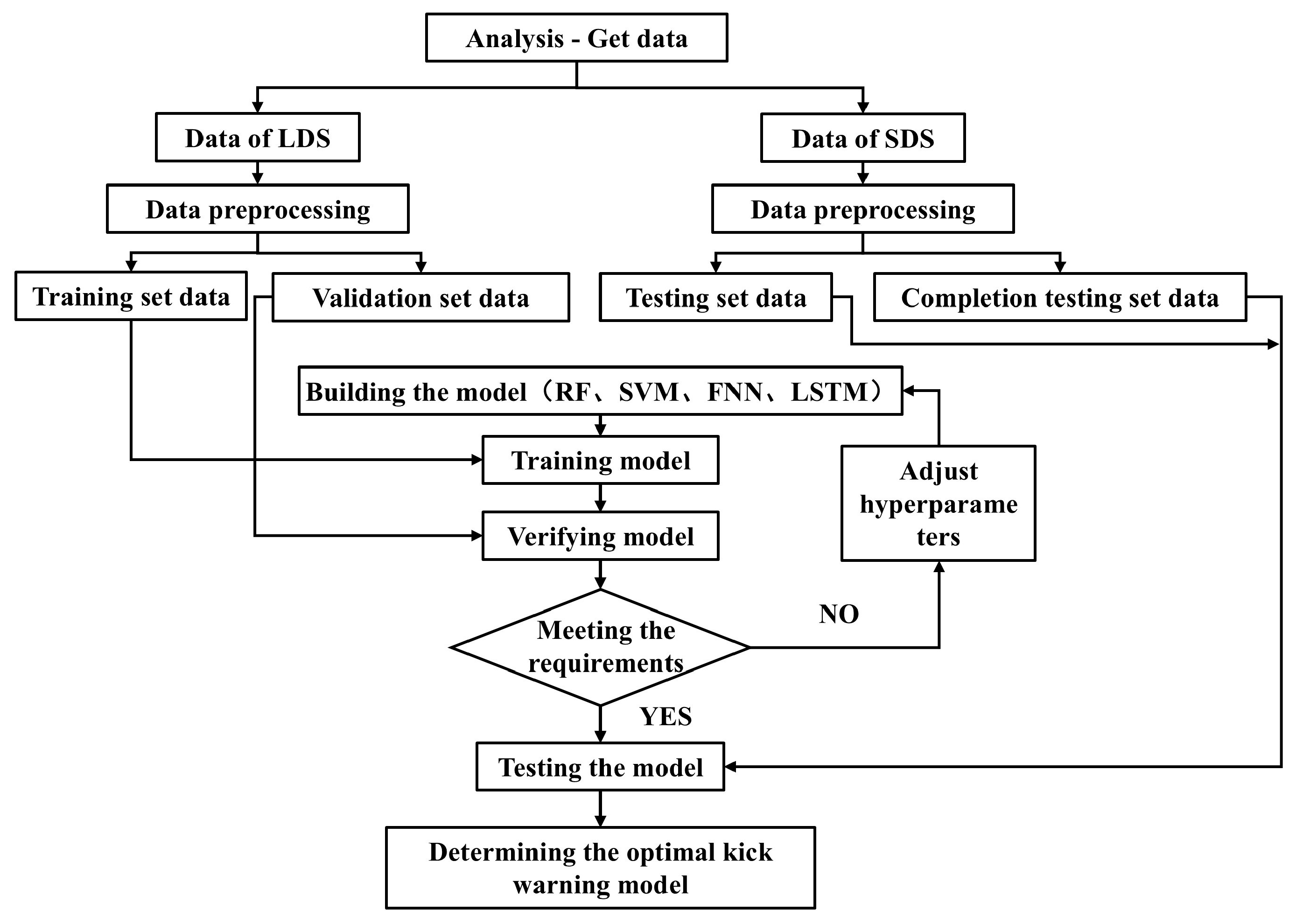
As illustrated in Figure 1, our methodology comprises the following:

Figure 1.
Flow chart of kick inversion.
Step 1: Analyze the causes of kick and the characteristic factors of kick, and theoretically preliminarily determine the parameters of kick early-warning model based on machine learning by evaluation indexes.
Step 2: Compare the obtained parameters with the analysis parameters in the first step, select/supplement parameters, determine the final characteristic parameters, preprocess the data, and determine the training set, verification set, and test set data required for the model establishment.
Step 3: Implement the model through Python programming 3.11.5, compare the verification results, and determine the optimal hyperparameters of each algorithm.
Step 4: Test the optimal model through the test set, and analyze the mechanism of the effects of different models.
Step 5: Determine the optimal kick warning model.
2. Analysis of Kick Characterization Parameters
2.1. Kick Mechanism
The fundamental cause of kick incidents is bottom hole pressure (BHP) falling below formation pressure. Multiple operational mechanisms contribute to this pressure imbalance [11,33].
For conventional oil fields: (1) Drilling design problem: Inaccurate prediction of formation pressure or underbalanced drilling; the density of drilling fluid is low, causing kick. (2) Loss of annulus pressure loss: Stopping the pump causes the loss of annulus pressure; the BHP is lower than the formation pressure to cause kick. (3) Swab pressure: When tripping, the upward movement of the drilling tool causes the BHP to decrease and kick. (4) The height of the drilling fluid column decreased: The drilling fluid was not injected into the wellbore in time during tripping to cause kick; when a lost circulation occurred, the height of the drilling fluid column decreased and caused the kick. (5) When the adjacent well is a water well, water injection development will artificially increase the formation pressure and cause formation fluids to invade the wellbore. (6) Other reasons are as follows: the drill bit drills into other wells; the gas-bearing sandstone is drilled quickly; underbalanced perforation or inaccurate perforation control BHP may make the BHP insufficient to balance the formation pressure, causing kick.
The predominant causal factors include inadequate wellbore filling during tripping up, excessive swab pressure, low mud density, abnormal formation pressures, and circulation loss [24].
The compressibility of gases and geological conditions such as carbonate rocks can lead to unique risk characteristics. Microscopic bubbles generated during drilling undergo significant volumetric expansion during ascent as pressure decreases. This continuously reduces equivalent circulating density (ECD), particularly in high-pressure formations, ultimately triggering kicks [37]. When the BHP is less than the formation pressure, (1) formation gas enters the wellbore under the action of pressure difference, causing kick; (2) the drill bit crushes the rock and the gas in the rock debris enters the wellbore, triggering kick; and (3) the formation gas enters under the action of the concentration difference, causing kick. The pressure difference is the main cause of kick. When the BHP is greater than or equal to the formation pressure, in addition to the above-mentioned crushed rock and concentration difference causing gas to enter the wellbore to cause kick, there are also density difference displacement gas and drilling and swabbing gas, and these two are the main reasons for kick. Especially when drilling into fractured reservoirs, kick occurs very easily for this reason.
2.2. Characteristic Parameters of Kick
Numerous studies have investigated kick characteristic parameters [11,37]. Based on kick manifestation mechanisms, indicators are categorized as direct or indirect symptoms:
- (1)
- Direct Symptom Parameters:
(1) Increased drilling fluid DF. (2) There are oil stains and air bubbles in the drilling fluid returned. (3) Changes in relevant parameters of drilling fluid: due to formation fluid invasion, drilling fluid density decreases; the conductivity of drilling fluid (CDF) increases due to the increase or decrease in monitored chlorine content (oil or gas invasion or freshwater entry); H2S concentration increases as gas composition changes in drilling fluid; C1 component increases (gas invasion) or decreases (oil invasion), but water invasion does not affect.
- (2)
- Indirect Symptom Parameters:
(1) Changes in weight on hook (WOH): formation fluid invasion leads to lower drilling fluid density and lowers buoyancy to drill string, which increases hook load; when the local fluid intrudes into the wellbore quickly, it is also possible to lift the drilling tool, thus reducing the hook load. (2) Pump pressure and riser pressure drop or rise briefly and then fall: due to fluid intrusion into the wellbore, annulus drilling fluid density drops, which will result in lower pump pressure and riser pressure based on the U-pipe principle; on the other hand, the formation pressure and the invasion of oil, gas, and water into the wellbore make the drilling fluid flocculate, thus causing the pump pressure or riser pressure to rise briefly and then fall. (3) The drilling speed increases sharply, the drilling pressure, torque, and drilling time decrease, and WOH rises sharply. In other words, the normal pressure layer is drilled into the abnormally high-pressure formation. Due to the insufficient compaction of the abnormally high-pressure formation, the drilling speed is accelerated, and the weight of bit (WOB) and torque are decreased. (4) Changes in the characteristics of returned cuttings: the returned cuttings change from small round and flat cuttings to larger and angular cuttings. (5) Change in bottom hole parameters: the annulus pressure in the bottom hole increases; bottom hole annulus temperature increases (oil or water invasion) or decreases (gas invasion).
2.3. Parameter Selection
To address prevalent wellsite challenges of delayed alarms, false positives, and missed detections, optimization of input data types is essential for enhancing alarm timeliness and reliability. Timeliness is the data delay time and data transmission time of sensor acquisition of survey data [38]. For the surface, the parameters include DFO, WOH, SPP, casing pressure, ROM, ROP (rate of penetration), torque, and so on. The required transmission time of these parameters is seconds. The mud pulse transmission method is widely used for downhole parameters at present. The transmission speed is 0.5–10 bit/s, and the pulse speed in the drilling fluid is 1200–1500 m/s. The time required for the pulse is generally between 20 and 97 s according to the mass of information and transmission distance. For credibility, to investigate and compare characteristic parameters of the common drilling complex accidents and the kick, Table 1 is established. The timeliness and credibility of the above parameters are analyzed: for the timeliness of 10 points in total, 1 point is deducted for increasing 10 s of response time; for the data credibility, the total score is 10 points, and 1 point is deducted for each additional disturbing working condition. The score calculation formula for each parameter is as follows and Table 2 is sorted by total points:

Table 1.
Changes in drilling accident parameters.
Table 2.
Kick parameter final score table.
DFO and ROP have a high score of 19, but the ROP data fluctuate greatly, so the ranking is lower than the DFO. The third place is torque and a series of 15-point parameters. The 15-point parameters are sorted according to the ease of data collection, including SPP, casing pressure, DDF, CDF, annulus pressure, bottom hole temperature, gas composition, and the last one is WOH.
3. Data Acquisition and Preprocessing
3.1. Data Acquisition
This paper analyzes two sets of experimental data from the Center for Risk, Integrity and Safety Engineering, Faculty of Engineering and Applied Sciences, Memorial University of Newfoundland. The first one was obtained using the small-scale drilling simulator (SDS) experiment reported by Islam et al. (2017) [39], and the second was obtained from the simulated well-kick experiment using the large-scale drilling simulator (LDS) [30]. The two drilling systems are similar, but the amount and method of the kick are different. SDS is powered by a 20 kW drill motor and operated manually; while LDS is powered by a 33 kW drill motor, and fully automatic control is achieved through a graphical user interface.
SDS well kick experiment: The experiment operation was tested in two different steps. The first step is to carry out an experimental operation without any air inflow to find safe operating limits. Three experiments were conducted under different pump flow rates to capture the working range of downhole parameter changes. The second step is to inject air within a predetermined period and perform the above three experiments again, keeping the pump flow rate almost the same as the three experiments in the first step.
LDS well kick experiment: During the drilling and circulation process of this experiment, when the drill bit grinds the synthetic rock sample fixed in place by the pressure drilling system and hits the area of high-pressure air, kick occurs. Before drilling, high-pressure air was trapped in a pre-drilled hole at the bottom of the synthetic rock sample. The gas is provided by a pneumatic kick injection system connected to the bottom of the drilling chamber.
The summary of SDS and LDS recording parameters is shown in Table 3. Because the fluid is not changed in the experiment, the outlet density parameter can be equivalently regarded as the DDF parameter.
Table 3.
SDS and LDS data summary table.
3.2. Data Preprocessing
3.2.1. Data Label
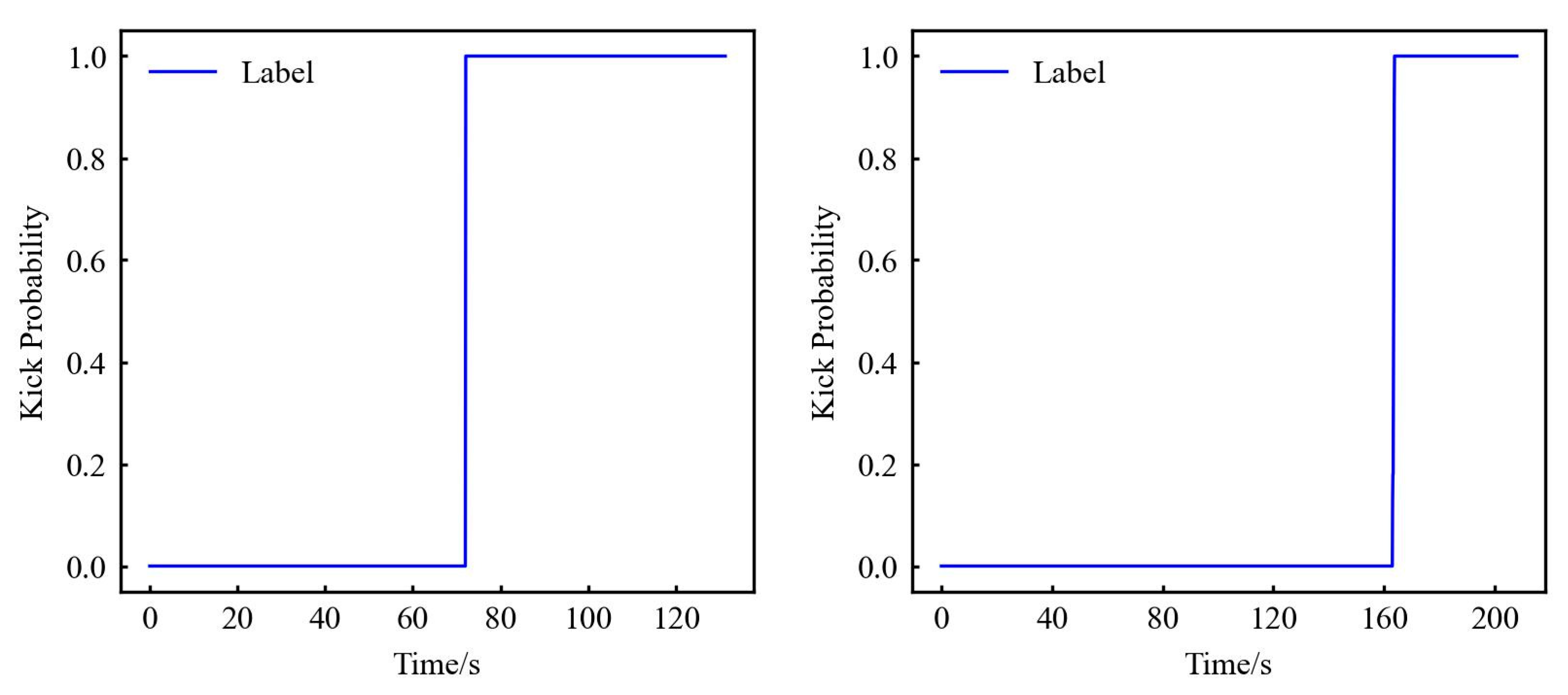
First set the label for the kick: Islam et al. [39] set the time of kick point about 70 s after the start of the experiment, and through comparison with the normal experiment, it can be judged that the data start the kick experiment at about 70 s. So, the labels of 0–70 s data are normal drilling data, and the data from 70 s and later are kick data (although the kick is stopped at about 124 s, considering that there is still gas rising, the label lasts until 130 s), labelled as shown in Figure 2. The LDS data begin the kick experiment at about 160 s, and the data thereafter are kick data, labelled as shown in Figure 2. The data label of kick is number 1; otherwise, the data label of non-kick is number 0. For specific data, please refer to the Supplementary Materials.
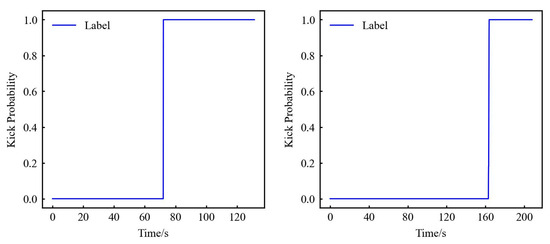
Figure 2.
SDS (left) and LDS (right) experiment result data label.
3.2.2. Data Completion
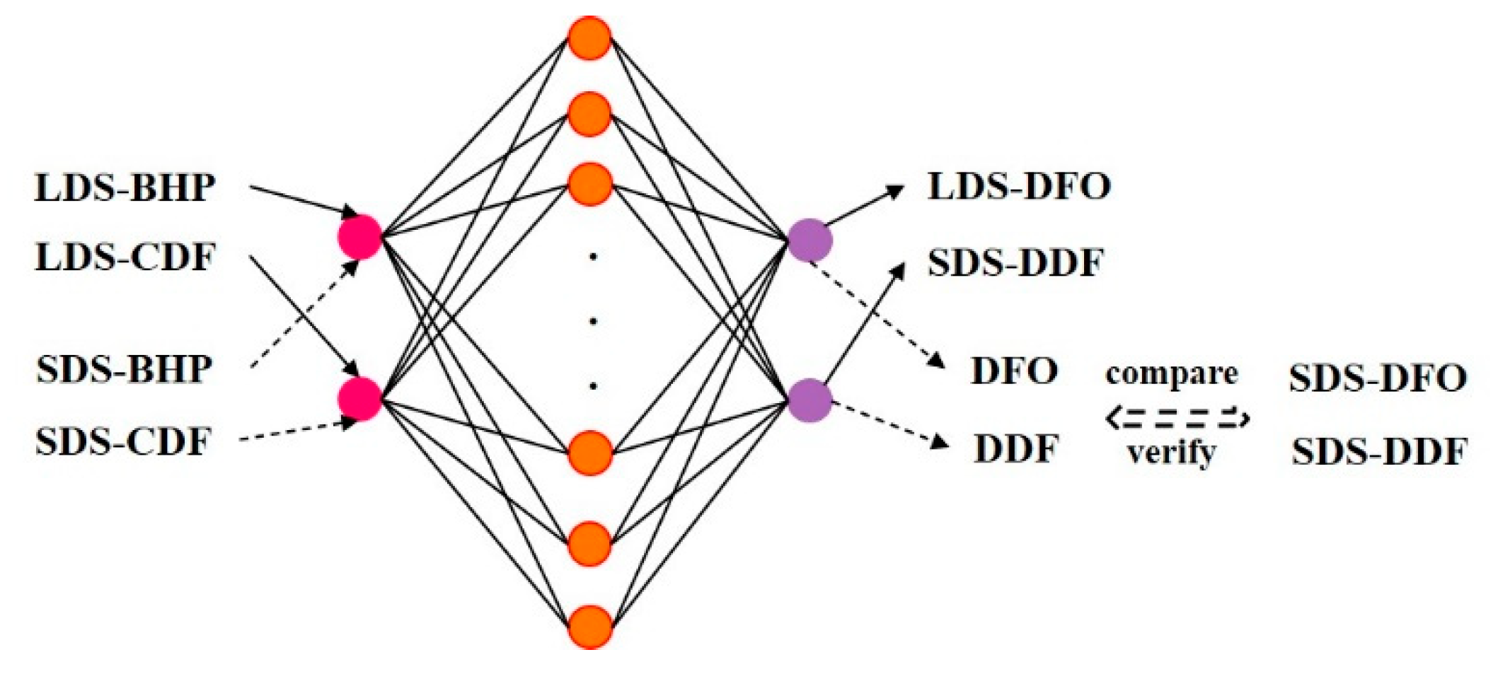
Due to parameter discrepancies between SDS and LDS data sets, models cannot be cross-tested. Among SDS parameters (DFO, BHP, DDF, CDF), only DFO scores highly, potentially skewing results. We address this via ① feature completion using fully connected neural networks (leveraging their strong approximation capabilities); ② restricted-input testing (only DFO/BHP/DDF/CDF).
For method ①: SDS torque, RPM, WOB, and GP (primarily surface parameters) are completed. To validate this approach, firstly, a training model with LDS downhole parameters (CDF/BHP) as inputs is used to predict surface parameters (DFO/DDF) (Figure 3 solid line). Secondly, inputting SDS CDF/BHP into trained model to compare outputs with actual SDS DFO/DDF (Figure 3 dashed line). This comparison evaluates the neural network’s drilling data completion efficacy.

Figure 3.
Schematic diagram of data completion principle.
Theoretically, increased neural network units/layers enable handling more complex problems. Given the data set’s simplicity, single-layer architectures with 200 or 500 units are selected. Hyperparameter selection used MSE loss and the Adam optimizer (Table 4), with training involving 200-epoch runs validated by 10-fold cross-testing. Results are averaged across tests. For regression performance, the coefficient of determination (R2) is employed. The final R-value represents the mean of R2 measurements for DFO and DDF parameters, with maximum R per parameter defining the optimal model (Table 5).
Table 4.
Data completion network parameter optimization.
Table 5.
Complete neural network results.
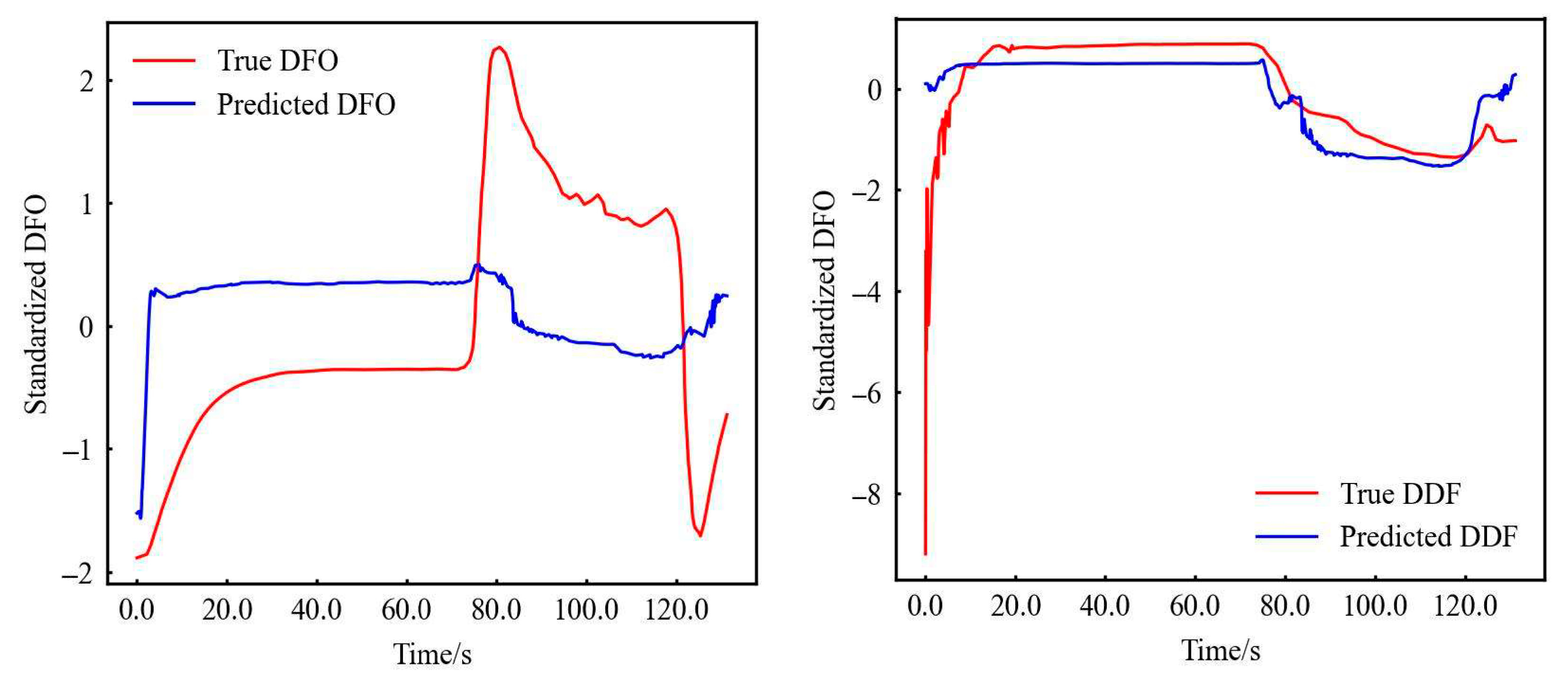
It can be seen that the above parameters with the best effect are standardization, 500 neurons, and tanh activation function. The fitting result is plotted as follows Figure 4.
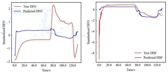
Figure 4.
Comparison of DFO (left) and DDF (right) completion results.
The kick detection relies on parameter trend analysis, which is prioritized trend fidelity over absolute value accuracy. Although true vs. predicted DFO values diverge significantly (Figure 4), the neural network perfectly captures its trend. This stems from DFO’s magnitude disparity versus other parameters: tanh activation compresses outputs to [−1, 1], impairing regression for values exceeding input scales. Therefore, when the input is the original value, R is the smallest, and the magnitude of adjustment (original value divided by 1000 decreases by three magnitudes) increases the R-value; for the other features (DDF) of the same order of magnitude as the input, not only the values after regression are similar, but the trend is captured completely.
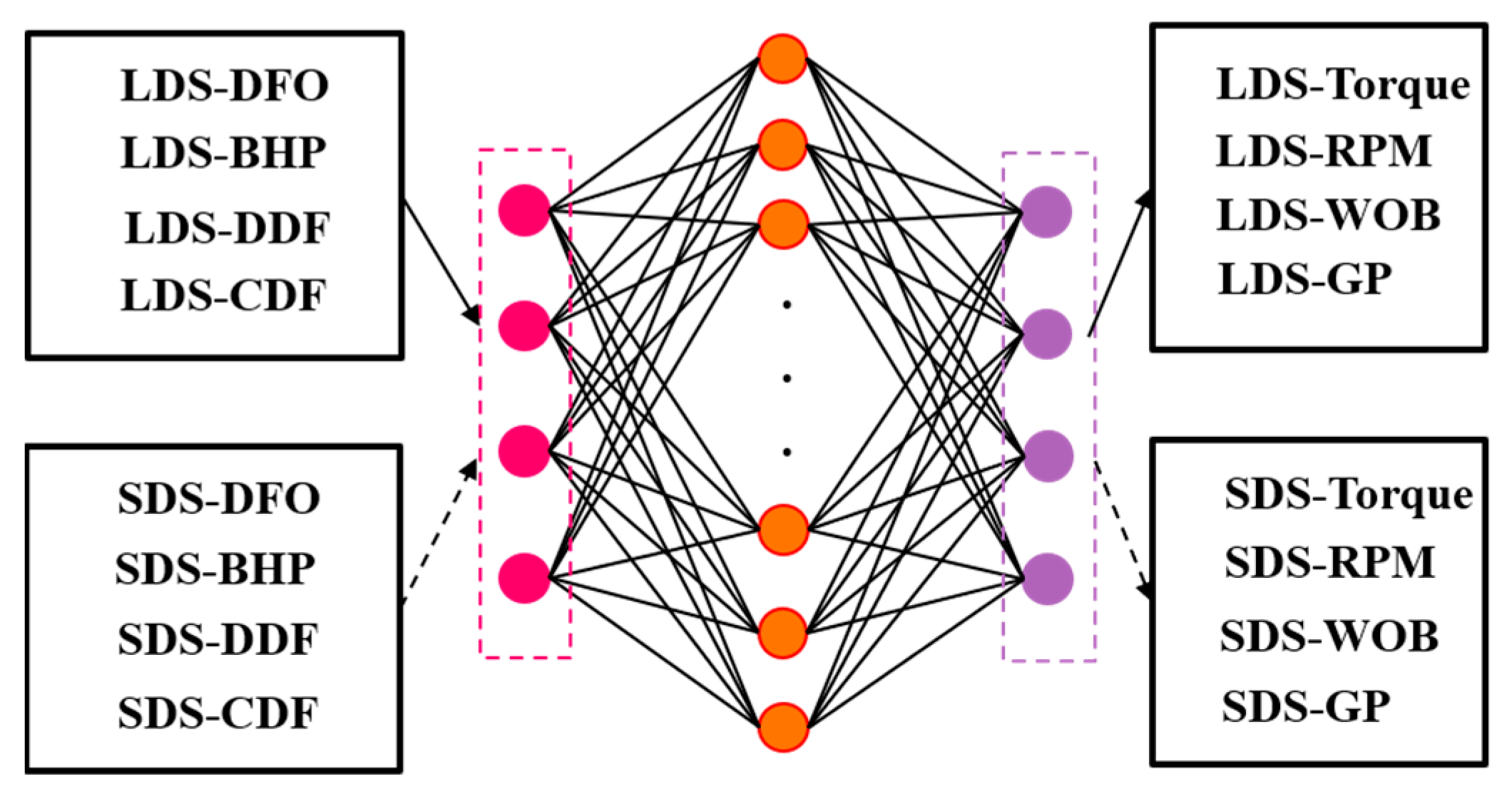
Therefore, this article finally decided to use 500 neurons, use the tanh activation function, Adam activation function, and train 1400 times, using the DFO, BHP, DDF, and CDF of the LDS data as input, and torque, GP, RPM, and WOB as output in the training model; bring the SDS data into the trained model to obtain the completed SDS data (CSDS data). The model structure is shown in Figure 5.
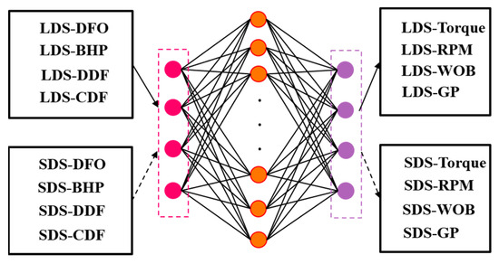
Figure 5.
SDS data completion.
3.2.3. Split Data Set
This paper divides the LDS data set 2:1 as the training set and the validation set; uses RF, SVM, FNN, and LSTM four algorithms to build the model; and uses all the SDS data as the test set to test the effectiveness of the model. At the same time, to test the effectiveness of the theoretical analysis feature selection, the standardized SDS original data and the CSDS data are used as the test set to compare the results.
The final data is shown in Table 6:
Table 6.
Introduction to SDS and LDS data.
4. Model Building and Results
4.1. Results Evaluation Indicators
For evaluating the classification results of a two-class problem, in addition to the commonly used accuracy rate (A), the evaluation indicators usually also consider four other criteria: recall rate (R), precision (P), false alarm rate (F), and missed alarm rate (M).
Accuracy (A) represents the proportion of samples that are classified correctly. The calculation formula is as follows:
where TP is the True Positives, TN is the True Negatives, FP is the False Positives, and FN is the False Negatives in the confusion matrix from the binary classified output of the FNN model. So, indicates the number of samples with positive labels classified into positive classes; indicates the number of samples with negative labels classified into negative classes; indicates the number of samples with negative labels classified as positive; and indicates the number of samples with positive labels classified as negative.
4.2. Algorithm Implementation and Model Optimization
This paper establishes four models, among which two models of RF and SVM are established by scikit-learn, and the FNN and LSTM using TensorFlow 2.12.0.
For the RF algorithm, the most important parameter is the number of trees in the forest. Generally, the higher the number of trees, the better the effect; the second is the maximum depth of the tree because when the number of experimental parameters is not high, the maximum depth is used; again, the minimum number of examples is of leaf nodes; indices of branching use Gini coefficients.
The two most important parameters for the SVM are the penalty term coefficient of the relaxation coefficient and the type of kernel function.
The important parameters of the FNN are the number of neurons and the activation function; the important parameter of LSTM is the number of neurons.
Table 7 details the hyperparameter optimization process for all algorithms.
Table 7.
Model hyperparameter adjustment.
4.2.1. Train and Validate the Model
Because there are two data sets, one is data with four characteristics after LDS (FLDS) data is standardized, the other is data with eight characteristics after LDS (ELDS) data is standardized, and two modeling verifications are performed. The optimal model of each algorithm is selected, and the optimal verification effects of the four models are as follows in Table 8. After finding the optimal model, SDS data and CSDS data will be used for testing.
Table 8.
Final verification of the four models.
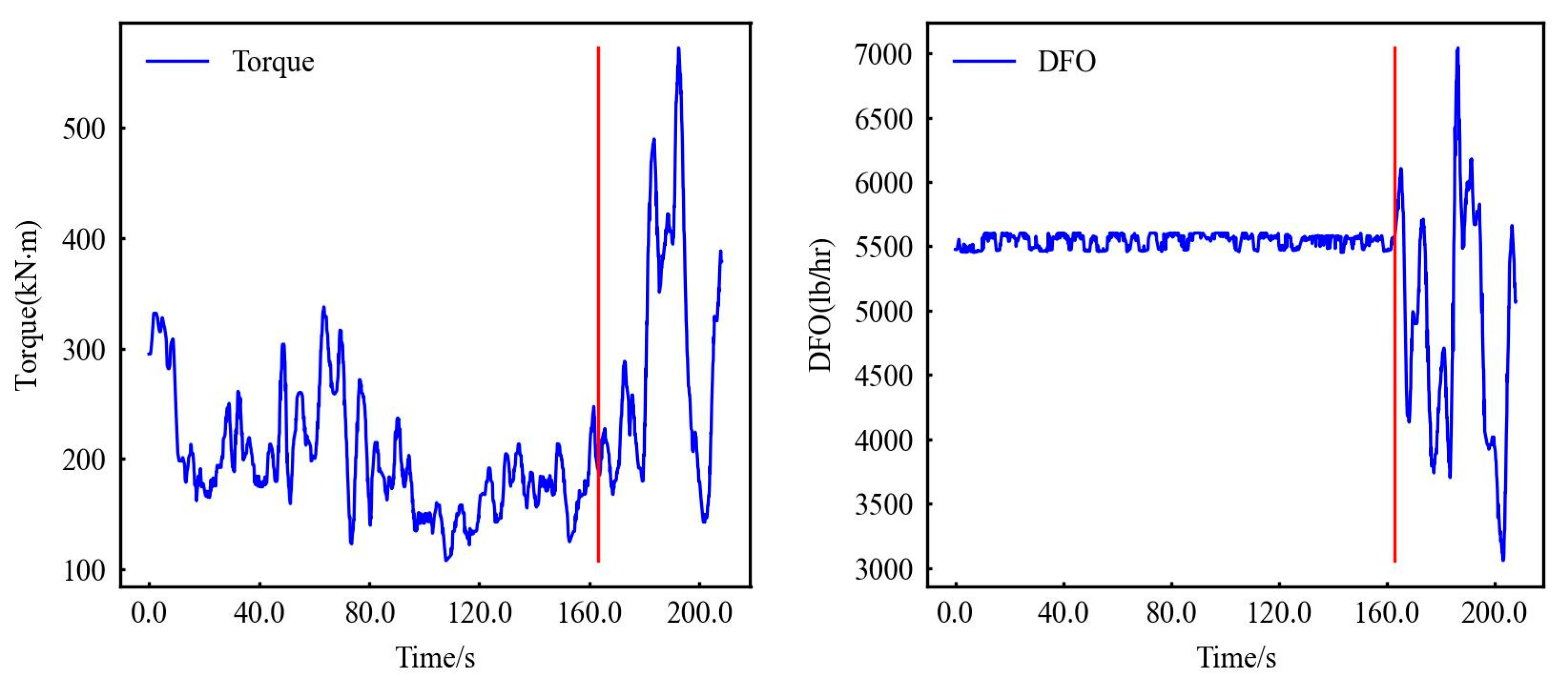
From the perspective of APRFM only, the four algorithm models after training and optimization using FLDS data have the same A and have the same M. It can be seen from Figure 6 and Figure 7 that the missed alarms are mainly caused by the lack of timely warning a few seconds after the kick occurs. The reason is mainly that among the input four characteristics, including DFO, BHP, DDF, and CDF, fluctuation exists. When the actual kick occurs, the short-term change is within the normal fluctuation range of the data, so there is no timely and accurate warning, which leads to missed alarms.
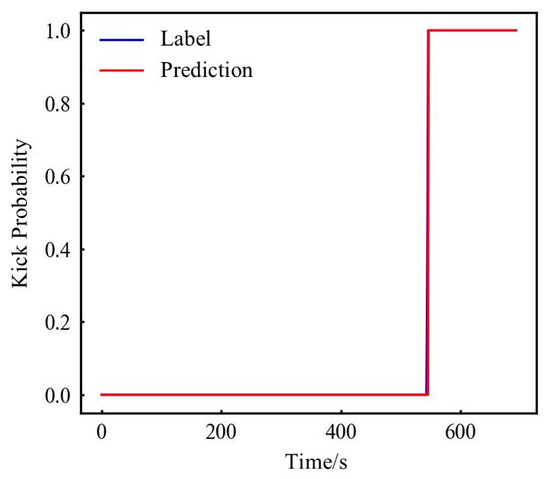
Figure 6.
Comparison of verification results.
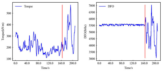
Figure 7.
LDS torque data and LDS DFO data. (Red line: Kick point).
Although the RF and SVM have reached 100% of the four algorithm models after training and optimization using the ELDS data, it does not mean that these two models are the best, nor can deny the FNN and LSTM models that do not reach 100%, because the risks of a model include experience risk and confidence risk. So far, it has been shown that RF and SVM perform better in experience risk. But in actual production, we tend to pay more attention to the confidence risk, that is, the performance of the trained model on the unknown data. Therefore, we used SDS data and CSDS data to test the above model.
4.2.2. Test the Model
Use the above-mentioned model, SDS data, and CSDS data to test, evaluate, and compare APRFM and alarm time results to determine the optimal model and clarify the optimal significance of the parameters.
- (1)
- The results of the APRFM are as follows Table 9.
Table 9. SDS data and CSDS data test results.
To analyze the stability of the model, all models were tested 10 times, and the best, worst and average results of APRMF were selected for display. In addition, the range, relative error, standard deviation, and coefficient of variation in the test results for 10 times judge the stability of the model effect. It can be seen from Table A1 that there is a certain gap in the completed model through the same training due to the influence of some initialized hyperparameters of RF, the FNN, and LSTM. In particular, the FNN model fluctuates the most. The accuracy of the SDS data and CSDS data fluctuates by about 0.03. From the point of view of 90% accuracy, the results of the FNN judged from the range, relative error, standard deviation, and coefficient of variation have not changed much. But the relative error is between −2.5% and 106.7% from the point of view of the M and F, and the maximum coefficient of variation is 1.789, the data fluctuate greatly. The specific reasons will be analyzed later. Compared with the FNN model with huge data fluctuations, the RF and LSTM models are relatively stable. The SVM model is classified due to its rigorous reasoning and is not affected by initialization, and the data results are the same.
To facilitate the analysis and display of the effects of the four models, the APRMF results of experiments 1, 2, and 3 of the ten tests are averaged and analyzed, as shown in Table 9. This article regards the A as the overall evaluation indicator, looking for models with low F and M and high P and R.
It can be seen from the evaluation indicators in Table 9 that when using the SDS data set for testing, both SVM-linear and the FNN have a higher A of 0.952, and the risks of missed and false alarms of both are lower. SVM-linear has an M of 0.064 and an F of 0.035; the FNN has an M of 0.102 and a F of 0.006. Although RF has a lower M (only 0.021), the F is as high as 0.106, and A is just 0.932. It can be seen that RF achieves a lower M by capturing more points, which may not have value for actual production because of higher F. While the LSTM model is relatively inferior to the SVM-linear and FNN models, the SVM-rbf model has the worst performance.
Bring CSDS data into the models to test and use the difference and the ratio of improvement relative to the SDS data to express the comparison effect as shown in Table 10. The specific calculation formula for the two is as follows:
Table 10.
Comparison of SDS data and CSDS data test results.
The results show that it can be found that the effects of SVM-linear and SVM-rbf are significantly improved, and the A is increased by 0.049 and 0.015, respectively. From Table 10, it can be seen that for the two models tested using CSDS data, the overall improvement effect of the two models, APR rises and MF falls. For the three models of RF, the FNN, and LSTM, the effect of adding features is not obvious from the overall evaluation (A). But in fact, it can be seen that due to the increase in the number of input parameter features, the model obtains more information, thereby reducing the tendency of the model to target a certain direction. Finally, the M and F of the model are close to the equilibrium direction, that is, the sensitivity of the model to overflow or non-overflow is weakened, and the generalization ability of the model is enhanced to a certain extent. However, compared with the other three models of the SVM model, the overall effect has not changed much, and the M and F have a balanced trend.
From the analysis of APRMF and result fluctuations, the optimal model should be the SVM-linear model, followed by the FNN model, LSTM model, SVM-rbf model, and the RF model. And the RF model has the lowest M and the highest F.
- (2)
- Warning time analysis
The timeliness of the kick warning is a very important issue. Although it does not need to be considered when it is 100% accurate, it is impossible to completely achieve 100%. Therefore, this article analyzes each time point.
The analysis mainly includes four-time periods before and after the kick time, namely the following:
(1) The period during which the data abruptly changes when the equipment is just running at the beginning of the experiment. This period simulates the drilling conditions when the pump turns on after the drilling is stopped for some uncertain reason. The abnormal situation during this period is a false alarm, and the recording time has a false alarm time of 0 (FT0). (2) The non-kick time after the data is stable. This period represents the normal drilling conditions. The abnormal situation during this period is a false alarm, and the recording time has a false alarm time of 1 (FT1). (3) After the kick occurs, the late time is the difference between the alarm time point and the actual kick time point. This period is the most important. It determines the response speed and how much time is left for the engineer to deal with the complicated time. The abnormal situation during this period is a late alarm, and the recording time is the late alarm time (LT). (4) The alarm stops when the kick still occurs. The abnormal situation during this period is the missed alarm, and the recording time is the missed alarm time (MT).
To analyze the above four periods of time, the two important time points are found. They are the turning point from the beginning of work to normal working conditions and the time point of kick. The time points of the three experiments are shown in Table 11.
Table 11.
Critical time.
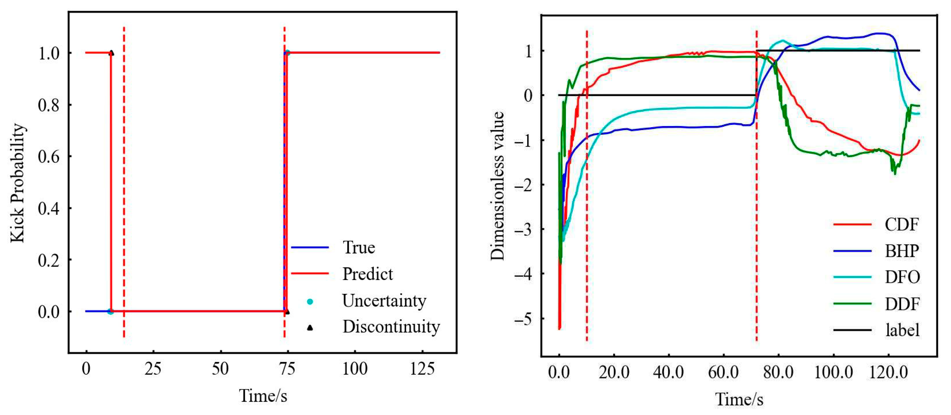
As mentioned earlier, the initialization of RF, the FNN, and LSTM has an impact on the model, which is reflected in the cyan dot named uncertainty point in Figure 8. It is due to the results of both kick and non-kick results in 10 tests. It can be seen from Figure 8 that this situation is more common in three locations: ① the time point when the experiment just started (0–14 s), ② the time point when the kick occurs (72–76 s), and ③ the time point when the experiment will end (122–124 s).
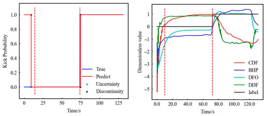
Figure 8.
Original data—RF test results (partial). (The first and second dotted red lines represent stable normal flow and the start of gas kick.)
Analyze the results of FT0, FT1, LT, and MT of the three experiments (see Table A2 for the specific data), and each kind of time has different meanings on the scene. In this paper, to comprehensively evaluate the actual effect of the model, the weighted average of each kind of time is carried out to obtain the comprehensive equivalent time (CET). The calculation formula is as follows:
where is the CET, s; is each kind of time in each case; and is the weight corresponding to each kind of time.
Using the above four periods of time and the CET, the FT0, FT1, LT, and MT are given weights of 2, 1, 5, and 3, respectively. The analysis of each model is shown in Table 12.
Table 12.
Test result analysis of time perspective.
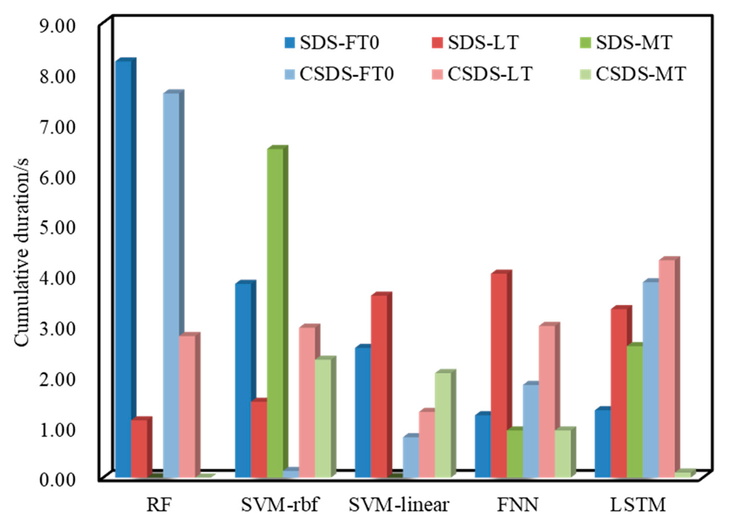
Since the FT1 of the SDS and CSDS data is 0, we will not analyze it in this article. Figure 9 shows a histogram drawn with FT0, FT1, LT, and MT. The dark color is the result of using the SDS data, and the light color is the result of using the CSDS data. The well site is most concerned about the LT. It can be seen from Figure 9 that in the model built using the SDS data, the LT increases sequentially; the highest is 4.03 s of the FNN, and the lowest is 1.13 s of RF. Secondly, the parameters of concern are the MT and the FT0. The MT of RF and SVM-linear are both 0, but the FT0 is relatively high, although the FNN has 0.93 s of MT and 1.23 s of the lowest FT.

Figure 9.
Test result analysis of time perspective.
Using the CSDS to test again, only SVM-linear and the FNN completed the original goal of CSDS data—reducing the LT, other models increase LT instead. The specific performance is that RF and SVM-rbf reduce the FT0 and MT, and the LT increases; LSTM reduces MT and the FT0 and the LT increases.
To facilitate analysis, list the comprehensive effective time histogram for analysis as follows in Figure 10. Analysis results of CET show that for the two types of input data, the SVM-linear model is the optimal model. The CET is 23.13 and 14.30, followed by the FNN’s 25.43 and 21.47.
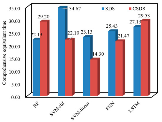
Figure 10.
The statistics of CET.
5. Analysis and Discussion
From the above results, it can be seen that for the kick simulation in the laboratory, the SVM-linear model has a good effect from the evaluation indicators to time analysis, followed by the FNN model. Through the analysis of the CSDS data, it is found that when the number of features increases, the model tends to balance between missed alarms with false alarms.
Due to the interpretability of RF and the SVM, we analyze the problem of model effect changes.
For RF, it can be seen from Table 13 that although theoretically increasing the timeliness characteristics to reduce the LT of the model, the decision tree established in the forest does not give very obvious weights to torque, RPM, and WOB, mainly because the experimental data transmission time difference is not large. And compared with the SDS data, adding features does not affect the weight of the original low-weight features, and more of the original key point feature weights are weakened. It can also be understood that the balancing phenomenon occurs because the weight of key nodes for missing or false alarms is reduced, and the weight of new features is increased.
Table 13.
The weights of different parameters in RF.
For the SVM, it is classified by selecting the support vector with label 0 and label 1, as shown in Table 14. For SVM-linear, the typical support vector for 22 non-kick states and 8 kick time points are selected; for SVM-rbf, 19 non-kick state points and 15 kick state points are selected. There are 15 identical support vectors for the two models, of which 9 are non-kick points and 6 are kick points. For the CSDS data, SVM-rbf also uses more support vectors, but the kick vector increases significantly. When the kick vector increases, the result is more likely to be biased toward kick. Therefore, it can be seen from Table 14 that the P and R of the SVM-rbf model established using CSDS data have increased significantly; for the SVM-linear established using CSDS data, although the total support vector is reduced, the non-kick vector is significantly reduced which is similar with the principle of kick vectors increase. So the result tends to kick and the P increases significantly.
Table 14.
SVM support vector analysis.
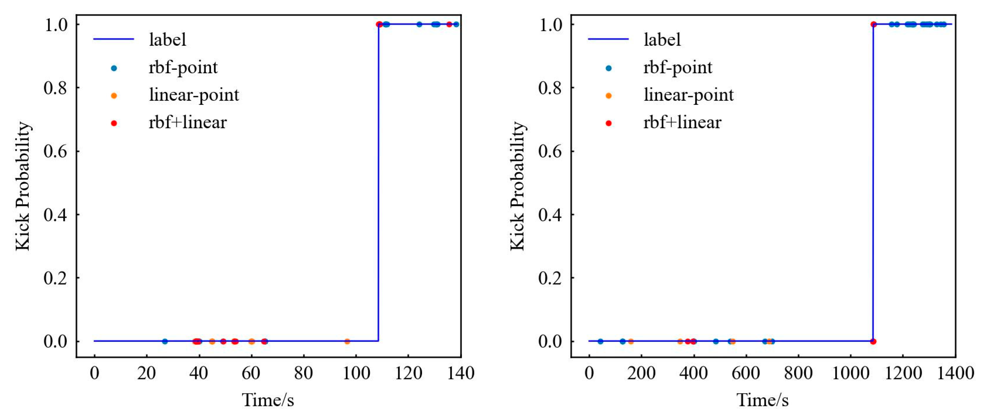
To understand the support vector situation more vividly, two SVM support vector points of two kinds of data are depicted. The most important point should be the non-overlapping points of the two models, that is, the blue and orange points in Figure 11. These points ultimately determine the root cause of the different model results. It can be seen from Figure 11 that these points are mainly distributed before 40 s and after 120 s. What is surprising is that the first one of these two values is very close to the time point when the experiment begins the steady process, and the second time point represents the time point when the experiment really ends. In fact, we modify the label, that is, when the label is shown in Figure 12, SVM-rbf becomes the best model. It can be seen that when the label is accurate, SVM-rbf should have a better effect on more complex data, but it is also due to the choice of a large number of support vectors that will increase the time-consuming training and verification. This is also one of the reasons why the SVM is suitable for small samples. It can also be seen that when the data complexity increases, the SVM-linear is weaker than the SVM-rbf model in Table 15 and Table 16.
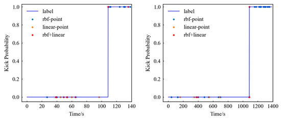
Figure 11.
SDS (left) and CSDS (right) data support vector analysis.
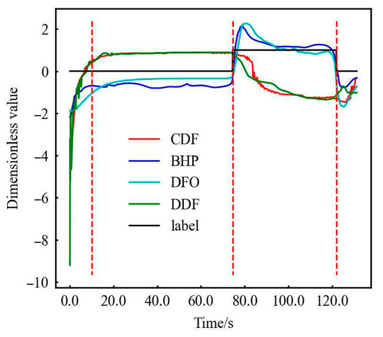
Figure 12.
SDS data characteristics after modifying the label. (The first, second and third red dotted lines represent the stable normal flow, the start and end points of gas kick.)
Table 15.
The SDS data and CSDS data test results after modifying the label.
Table 16.
Comparison of the original data and the CSDS data test results after modifying the label.
For the FNN model and the LSTM model, it is difficult to analyze the neural network due to the inexplicability of the neural network. However, according to the calculation process of the neural network, the neural network itself can reduce noise. When new features are introduced, the neural network proposes the internal correlation between the features and the kick. When the number of features increases, the increase in information obtained by the neural network reduces the development of the neural network in a certain direction (missed or false alarm). The specific principle can be roughly understood as the correction of the feature weight distribution of RF, so that the neural network result also tends to be balanced status.
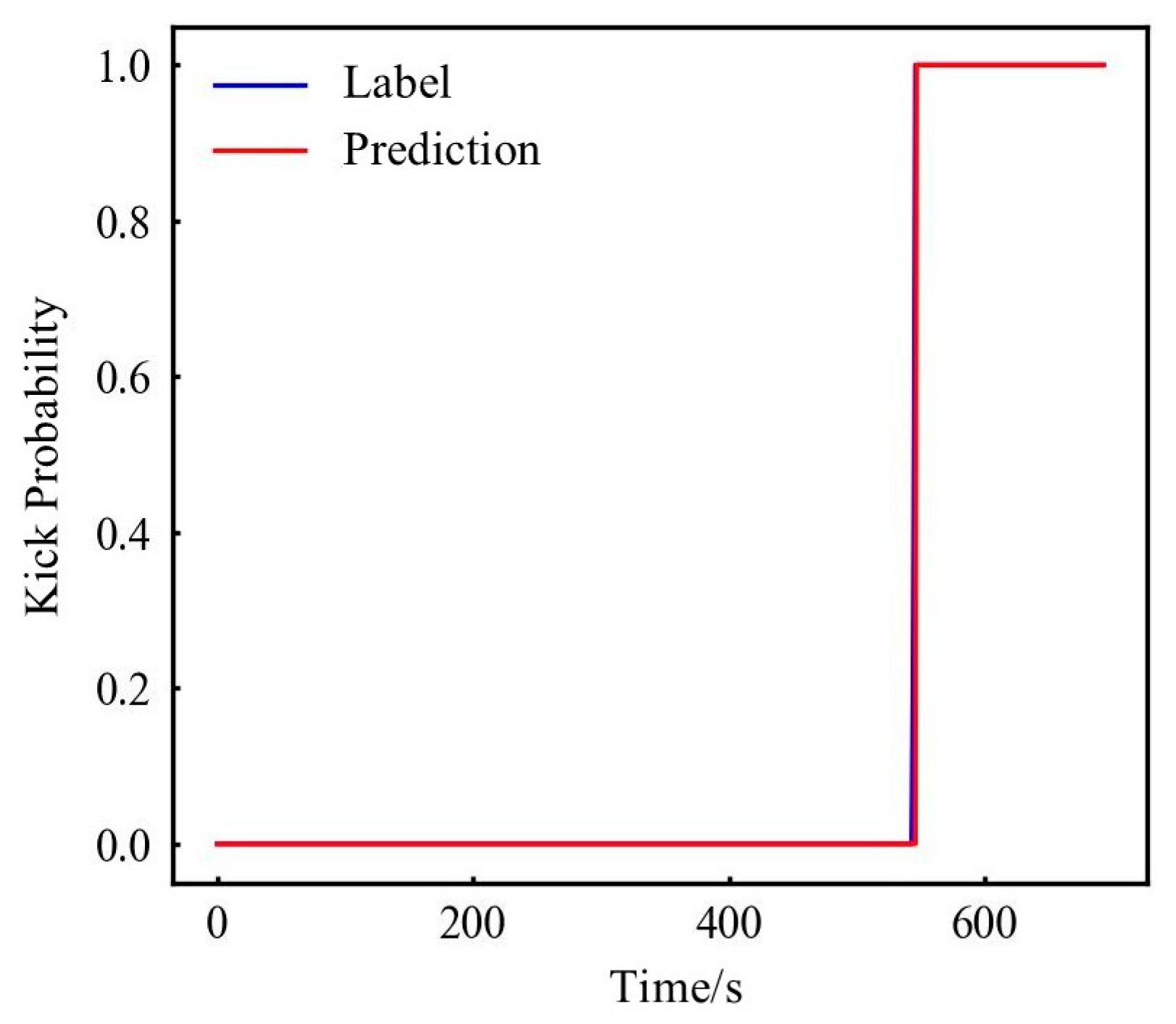
In addition, for the neural network, especially the FNN model, the data fluctuates sharply. The above analysis only uses the average value of the evaluation indicators for comparison. The ensemble thought can also be used. Count the results of 10 tests and give an early warning when the response threshold is exceeded. For example, if the threshold is 0.5, more than 50% of network warnings are true warnings, as shown in Figure 13. Early warning is given in the part above the blue dotted line in Figure 13, and no warning is given in the following part. This paper uses 0.3, 0.5, and 0.7 to analyze again, and the results are as follows in Table 17.

Figure 13.
The FNN predicts the probability curve of kick after modifying the label. (The first and second dotted red lines represent stable normal flow and the start of gas kick.)
Table 17.
The FNN predicts different threshold evaluation indicators of kick after modifying the label.
From Table 17, it can be seen that after ensemble, the model effect has been improved from the evaluation indicators, and the model stability has been strengthened, but it is still slightly inferior to the fully stable SVM model. From the CET analysis in Table 18, it is found that a higher threshold value needs to be set when there are fewer features, and a smaller threshold value needs to be set when there are more features, and the model performance is better than the SVM model when the threshold value is appropriate. The reason may be that less information can be obtained when there are fewer features, and more votes are needed to ensure the correct result; but when there are too many features, effective information is added and noise increases, and it is necessary to vote for certain sensitive features to improve results.
Table 18.
After modifying the label, the FNN predicts different threshold time indicators of kick.
At the same time, according to the evaluation indicators and time analysis, it can be seen that for a certain neural network model, when the data have similar characteristic data (SDS data and CSDS data), its performance is relatively stable. Its accuracy fluctuates less than 0.05%, and the CET fluctuates less than 4 s. And the FNN and LSTM are only slightly inferior to the SVM model, but the effect may be better than the SVM model after ensemble.
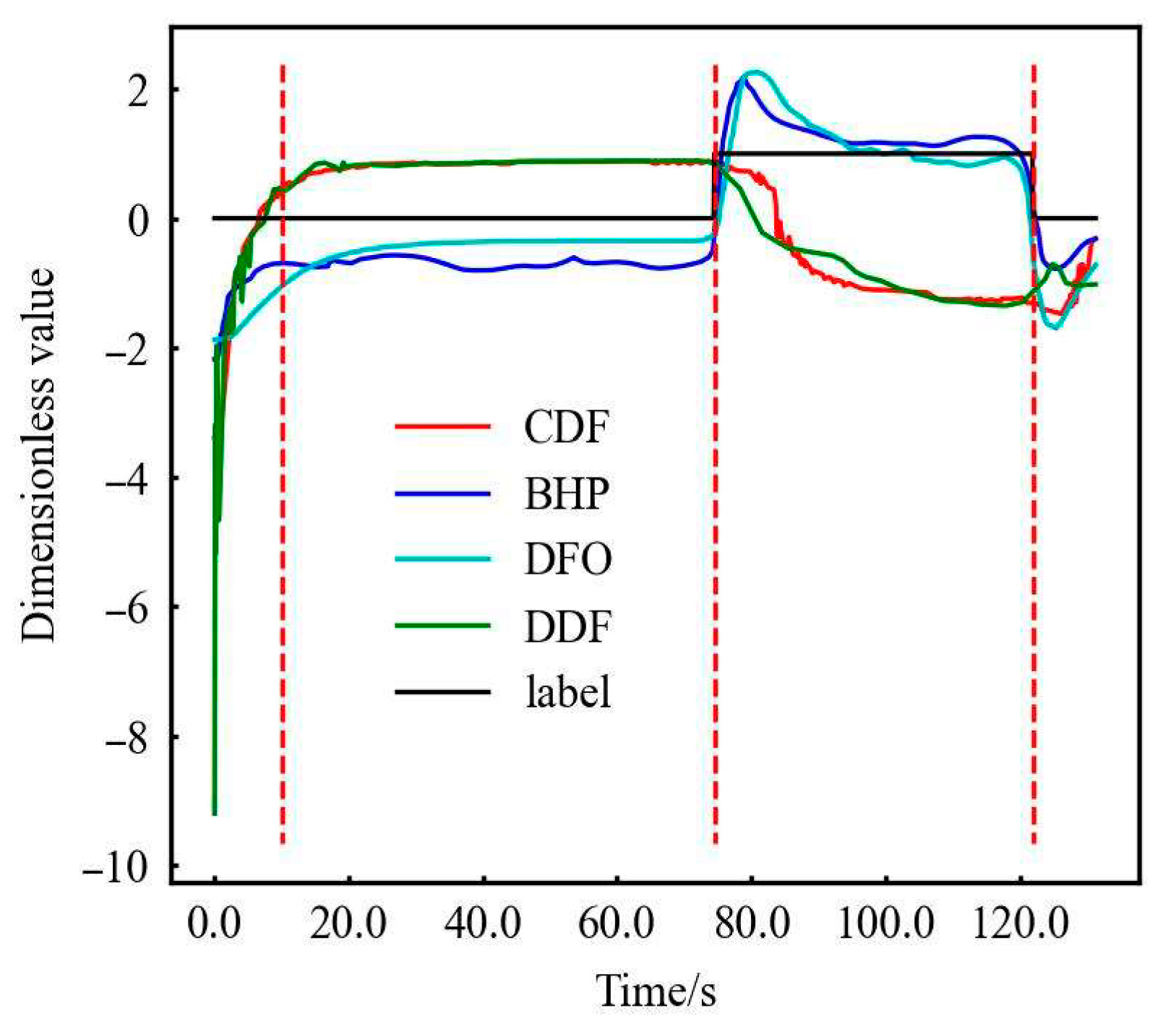
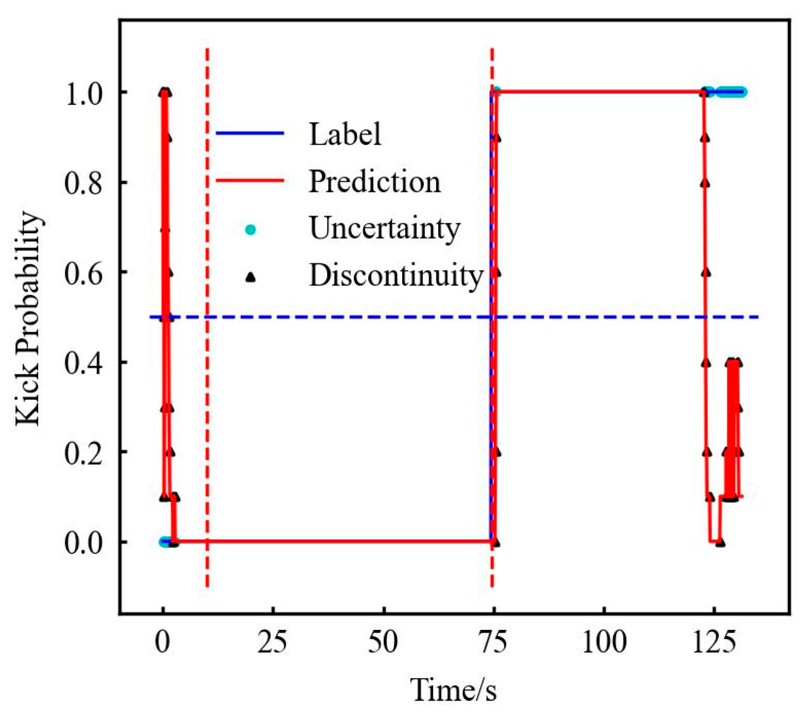
This paper utilizes authentic mud logging data sourced from Duan et al. [40] to further test the model using CDF, BHP, DFO, and DDF parameters. Figure 14 demonstrates that alerts are triggered 2 min earlier than logging timestamps.
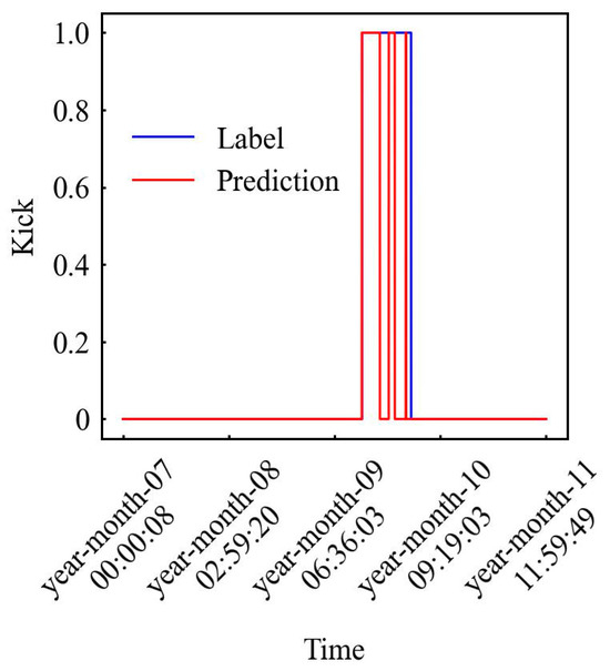
Figure 14.
Model on-site data verification results.
The paper developed a neural network-based data imputation method to address data gaps. Through comparative model analysis, the SVM algorithm was selected for optimization. The constructed SVM-linear model is trained on small gas kick samples, which enables rapid model deployment (<5 min) and effective gas kick detection, resolving challenges of limited on-site risk cases and protracted modeling timelines.
However, the process of integrating this model with field data requires further development, and it has not yet accounted for formation effects. Both limitations stem from constraints in the available field data. Future work will necessitate leveraging historical and real-time field data for more extensive validation to enhance model accuracy and analyze its generalization capabilities.
6. Conclusions
This article preliminarily selects the types of kick parameters by analyzing the mechanism and characterization parameters of kick. It establishes RF, SVM-rbf, SVM-linear, FNN, LSTM models through LDS data, optimize hyperparameters, and uses SDS and CSDS data for testing. The evaluation was conducted through evaluation indicators and CET, and the results showed the following:
- Although from theoretical analysis, parameters such as DOF, torque, and DDF contribute to the improvement of the model, the effect of actual data indicates that its effect may not be obvious during application.
- Use experimental data to test RF, the SVM, FNN, and LSTM to train, verify, and test models. The results show that the above models are evaluated by APRMF and CET. Among them, the SVM-linear model can achieve the highest accuracy rate of 0.968 and only has the M of 0.06 and the F of 0.11. The LT is 1.3 s, and the CET is 23.13. The effect of the SVM-linear model is the best. However, when using complex data, the effect of the slightly worse SVM-rbf model may exceed the SVM-linear model. The FNN and LSTM models are slightly inferior to the SVM model, but they also have an accuracy of about 0.950 and the two models are more stable for different data, and the ensemble model effect may be better than the SVM model. The RF model has an accuracy of only about 0.900, which is the worst overall.
- This article analyzes the reason for the different performance of the four models after adding features: RF reduces the original high-weight features and assigns new feature weights to increase the available information of the model. The result tends to balance the M and F; the SVM model improves the model effect by changing the number of kick and non-kick vectors, especially focusing on the vectors near the special points; the neural network extracts new feature information to balance false alarms and missed alarm, on the one hand, and keep the model stable on the other hand.
- In the comparison of the four models, the SVM model has the best effect (accuracy rate of 0.968), but it has the hidden danger of reduced effect due to complex training data. The ensemble FNN model is slightly inferior or slightly better than the SVM (accuracy rate is about 0.950) model, but it has good stability.
The paper selected an optimized SVM model for its superior efficiency and accuracy. Utilizing historical logging data, the model successfully generated kick alerts two minutes ahead of recorded alarm events. This model is expected to provide faster and more accurate kick warnings at the drilling site, enabling timely risk mitigation and enhanced drilling safety.
Supplementary Materials
The following supporting information can be downloaded at: https://www.mdpi.com/article/10.3390/pr13072162/s1, Excel S1: LDS kick data; Excel S2: SDS kick data; Excel S3: SDS normal data.
Author Contributions
Conceptualization, C.L. and Z.Z.; methodology, C.L., Z.Z. and Y.C.; software, S.D.; validation, H.W. and Z.X.; formal analysis, C.L., Z.Z. and Y.C.; investigation, C.L., Z.Z. and H.W.; resources, C.L. and Z.Z.; data curation, C.L., Z.Z., Y.C. and Y.C.; writing—original draft preparation, C.L., Z.Z. and Y.C.; writing—review and editing, C.L., Z.Z. and M.Z.; visualization, H.W. and M.Z.; supervision, Z.Z. and M.Z.; project administration, Z.Z. and M.Z.; funding acquisition, Z.Z. All authors have read and agreed to the published version of the manuscript.
Funding
The authors would like to acknowledge the project supported by the Youth Foundation of National Natural Science Foundation of China (No. 52204020).
Data Availability Statement
The data presented in this study are available on request from the corresponding author. Because the field data are not publicly available due to privacy or ethical restrictions.
Conflicts of Interest
Author C.L. were employed by the company Sinopec. The remaining authors declare that the research was conducted in the absence of any commercial or financial relationships that could be construed as a potential conflict of interest.
Nomenclature
| A | Accuracy |
| BHP | Bottom Hole Pressure |
| CDF | Conductivity of Drilling Fluid |
| DDF | Density of Drilling Fluid |
| DF | Differential Flow |
| F | Missed Alarm Rate |
| FNN | Fully Connected Neural Network |
| GP | Gas Pressure |
| LDS | Large-scale Drilling Simulator |
| LSTM | Long Short-term Memory Neural Network |
| M | False Alarm Rate |
| P | Precision |
| R | Recall Rate |
| RF | Random Forest |
| ROP | Rate Of Penetration |
| RPM | Rate Per Minute |
| SDS | Small-scale Drilling Simulator |
| SPP | Standpipe Pressure |
| SVM | Support Vector Machine |
| SVM-linear | SVM using Linear Kernel Function |
| SVM-rbf | SVM using RBF Kernel Function |
| WOB | Weight On Bit |
| WOH | Weight On Hook |
| Parameter Timeliness Score | |
| Parameter Credibility Score | |
| Parameter Total Score |
Appendix A
Table A1.
Extreme value, audit, relative error, standard deviation, and coefficient of variation.
Table A1.
Extreme value, audit, relative error, standard deviation, and coefficient of variation.
| Model | Experiment | Indicators | SDS Data | CSDS Data | ||||||||
|---|---|---|---|---|---|---|---|---|---|---|---|---|
| A | P | R | M | F | A | P | R | M | F | |||
| RF | First | max | 0.942 | 0.982 | 0.894 | 0.137 | 0.021 | 0.932 | 0.982 | 0.876 | 0.124 | 0.015 |
| min | 0.922 | 0.975 | 0.863 | 0.106 | 0.015 | 0.932 | 0.982 | 0.876 | 0.124 | 0.015 | ||
| max-min | 0.020 | 0.007 | 0.031 | 0.031 | 0.006 | 0.000 | 0.000 | 0.000 | 0.000 | 0.000 | ||
| error | 0.021 | 0.007 | 0.035 | 0.228 | 0.304 | 0.000 | 0.000 | 0.000 | 0.000 | 0.000 | ||
| std | 0.009 | 0.002 | 0.015 | 0.015 | 0.002 | 0.000 | 0.000 | 0.000 | 0.000 | 0.000 | ||
| cv | 0.009 | 0.003 | 0.017 | 0.125 | 0.112 | 0.000 | 0.000 | 0.000 | 0.000 | 0.000 | ||
| Second | max | 0.941 | 0.976 | 0.900 | 0.103 | 0.024 | 0.925 | 0.933 | 0.904 | 0.107 | 0.058 | |
| min | 0.938 | 0.973 | 0.897 | 0.100 | 0.021 | 0.919 | 0.933 | 0.893 | 0.096 | 0.057 | ||
| max-min | 0.003 | 0.003 | 0.003 | 0.003 | 0.003 | 0.005 | 0.000 | 0.010 | 0.010 | 0.001 | ||
| error | 0.003 | 0.003 | 0.003 | 0.030 | 0.125 | 0.006 | 0.000 | 0.011 | 0.096 | 0.010 | ||
| std | 0.001 | 0.001 | 0.001 | 0.001 | 0.001 | 0.002 | 0.000 | 0.004 | 0.004 | 0.000 | ||
| cv | 0.001 | 0.001 | 0.001 | 0.008 | 0.041 | 0.002 | 0.000 | 0.005 | 0.042 | 0.004 | ||
| Third | max | 0.926 | 0.984 | 0.866 | 0.141 | 0.018 | 0.920 | 0.936 | 0.888 | 0.140 | 0.054 | |
| min | 0.922 | 0.979 | 0.859 | 0.134 | 0.014 | 0.905 | 0.936 | 0.860 | 0.112 | 0.052 | ||
| max-min | 0.004 | 0.005 | 0.007 | 0.007 | 0.004 | 0.015 | 0.000 | 0.028 | 0.028 | 0.002 | ||
| error | 0.004 | 0.005 | 0.008 | 0.047 | 0.247 | 0.017 | 0.000 | 0.032 | 0.202 | 0.028 | ||
| std | 0.002 | 0.002 | 0.003 | 0.003 | 0.001 | 0.007 | 0.000 | 0.014 | 0.014 | 0.001 | ||
| cv | 0.002 | 0.002 | 0.003 | 0.022 | 0.094 | 0.008 | 0.000 | 0.016 | 0.106 | 0.014 | ||
| SVM | First | max | 0.949 | 0.968 | 0.918 | 0.082 | 0.025 | 0.958 | 0.942 | 0.961 | 0.039 | 0.044 |
| min | 0.949 | 0.968 | 0.918 | 0.082 | 0.025 | 0.958 | 0.942 | 0.961 | 0.039 | 0.044 | ||
| max-min | 0.000 | 0.000 | 0.000 | 0.000 | 0.000 | 0.000 | 0.000 | 0.000 | 0.000 | 0.000 | ||
| error | 0.000 | 0.000 | 0.000 | 0.000 | 0.000 | 0.000 | 0.000 | 0.000 | 0.000 | 0.000 | ||
| std | 0.000 | 0.000 | 0.000 | 0.000 | 0.000 | 0.000 | 0.000 | 0.000 | 0.000 | 0.000 | ||
| cv | 0.000 | 0.000 | 0.000 | 0.000 | 0.000 | 0.000 | 0.000 | 0.000 | 0.000 | 0.000 | ||
| Second | max | 0.957 | 0.921 | 0.984 | 0.016 | 0.062 | 0.957 | 0.907 | 0.996 | 0.004 | 0.071 | |
| min | 0.957 | 0.921 | 0.984 | 0.016 | 0.062 | 0.957 | 0.907 | 0.996 | 0.004 | 0.071 | ||
| max-min | 0.000 | 0.000 | 0.000 | 0.000 | 0.000 | 0.000 | 0.000 | 0.000 | 0.000 | 0.000 | ||
| error | 0.000 | 0.000 | 0.000 | 0.000 | 0.000 | 0.000 | 0.000 | 0.000 | 0.000 | 0.000 | ||
| std | 0.000 | 0.000 | 0.000 | 0.000 | 0.000 | 0.000 | 0.000 | 0.000 | 0.000 | 0.000 | ||
| cv | 0.000 | 0.000 | 0.000 | 0.000 | 0.000 | 0.000 | 0.000 | 0.000 | 0.000 | 0.000 | ||
| Third | max | 0.951 | 0.920 | 0.965 | 0.035 | 0.060 | 0.988 | 0.972 | 1.000 | 0.000 | 0.021 | |
| min | 0.951 | 0.920 | 0.965 | 0.035 | 0.060 | 0.988 | 0.972 | 1.000 | 0.000 | 0.021 | ||
| max-min | 0.000 | 0.000 | 0.000 | 0.000 | 0.000 | 0.000 | 0.000 | 0.000 | 0.000 | 0.000 | ||
| error | 0.000 | 0.000 | 0.000 | 0.000 | 0.000 | 0.000 | 0.000 | 0.000 | 0.000 | 0.000 | ||
| std | 0.000 | 0.000 | 0.000 | 0.000 | 0.000 | 0.000 | 0.000 | 0.000 | 0.000 | 0.000 | ||
| cv | 0.000 | 0.000 | 0.000 | 0.000 | 0.000 | 0.000 | 0.000 | 0.000 | 0.000 | 0.000 | ||
| FNN | First | max | 0.954 | 0.938 | 0.990 | 0.046 | 0.114 | 0.968 | 0.986 | 0.950 | 0.085 | 0.064 |
| min | 0.920 | 0.833 | 0.954 | 0.010 | 0.046 | 0.941 | 0.914 | 0.915 | 0.050 | 0.011 | ||
| max-min | 0.033 | 0.105 | 0.036 | 0.036 | 0.067 | 0.027 | 0.072 | 0.035 | 0.035 | 0.053 | ||
| error | 0.035 | 0.112 | 0.036 | 0.775 | 0.592 | 0.028 | 0.073 | 0.037 | 0.410 | 0.824 | ||
| std | 0.009 | 0.031 | 0.010 | 0.010 | 0.020 | 0.008 | 0.024 | 0.011 | 0.011 | 0.018 | ||
| cv | 0.010 | 0.036 | 0.010 | 0.429 | 0.195 | 0.008 | 0.025 | 0.012 | 0.171 | 0.777 | ||
| Second | max | 0.973 | 0.939 | 1.000 | 0.013 | 0.086 | 0.969 | 0.944 | 0.986 | 0.031 | 0.078 | |
| min | 0.944 | 0.887 | 0.987 | 0.000 | 0.048 | 0.942 | 0.899 | 0.969 | 0.014 | 0.044 | ||
| max-min | 0.029 | 0.052 | 0.013 | 0.013 | 0.038 | 0.027 | 0.046 | 0.017 | 0.017 | 0.034 | ||
| error | 0.030 | 0.056 | 0.013 | 1.000 | 0.446 | 0.027 | 0.048 | 0.017 | 0.543 | 0.435 | ||
| std | 0.007 | 0.013 | 0.004 | 0.004 | 0.009 | 0.008 | 0.015 | 0.006 | 0.006 | 0.011 | ||
| cv | 0.007 | 0.014 | 0.004 | 1.789 | 0.144 | 0.009 | 0.016 | 0.006 | 0.275 | 0.172 | ||
| Third | max | 0.976 | 0.944 | 1.000 | 0.008 | 0.064 | 0.966 | 0.948 | 0.973 | 0.055 | 0.061 | |
| min | 0.959 | 0.913 | 0.992 | 0.000 | 0.042 | 0.941 | 0.920 | 0.945 | 0.027 | 0.040 | ||
| max-min | 0.017 | 0.031 | 0.008 | 0.008 | 0.022 | 0.024 | 0.028 | 0.029 | 0.029 | 0.021 | ||
| error | 0.017 | 0.033 | 0.008 | 1.000 | 0.348 | 0.025 | 0.029 | 0.029 | 0.516 | 0.348 | ||
| std | 0.004 | 0.008 | 0.002 | 0.002 | 0.006 | 0.007 | 0.010 | 0.010 | 0.010 | 0.007 | ||
| cv | 0.004 | 0.009 | 0.002 | 2.409 | 0.100 | 0.008 | 0.011 | 0.010 | 0.239 | 0.130 | ||
| LSTM | First | max | 0.921 | 0.859 | 0.964 | 0.047 | 0.113 | 0.966 | 0.984 | 0.945 | 0.082 | 0.045 |
| min | 0.915 | 0.837 | 0.953 | 0.036 | 0.100 | 0.951 | 0.940 | 0.918 | 0.055 | 0.013 | ||
| max-min | 0.006 | 0.023 | 0.011 | 0.011 | 0.014 | 0.015 | 0.044 | 0.027 | 0.027 | 0.033 | ||
| error | 0.007 | 0.027 | 0.011 | 0.233 | 0.119 | 0.016 | 0.045 | 0.029 | 0.333 | 0.724 | ||
| std | 0.002 | 0.006 | 0.004 | 0.004 | 0.004 | 0.004 | 0.013 | 0.009 | 0.009 | 0.010 | ||
| cv | 0.002 | 0.007 | 0.004 | 0.085 | 0.034 | 0.005 | 0.013 | 0.009 | 0.123 | 0.580 | ||
| Second | max | 0.963 | 0.931 | 0.991 | 0.018 | 0.067 | 0.947 | 0.927 | 0.978 | 0.051 | 0.098 | |
| min | 0.955 | 0.914 | 0.982 | 0.009 | 0.055 | 0.922 | 0.874 | 0.949 | 0.022 | 0.058 | ||
| max-min | 0.008 | 0.017 | 0.009 | 0.009 | 0.012 | 0.024 | 0.054 | 0.028 | 0.028 | 0.039 | ||
| error | 0.008 | 0.018 | 0.009 | 0.486 | 0.183 | 0.026 | 0.058 | 0.029 | 0.560 | 0.402 | ||
| std | 0.003 | 0.006 | 0.002 | 0.002 | 0.004 | 0.008 | 0.016 | 0.009 | 0.009 | 0.012 | ||
| cv | 0.003 | 0.007 | 0.002 | 0.178 | 0.075 | 0.008 | 0.018 | 0.009 | 0.216 | 0.136 | ||
| Third | max | 0.963 | 0.932 | 0.991 | 0.034 | 0.060 | 0.945 | 0.931 | 0.955 | 0.069 | 0.067 | |
| min | 0.951 | 0.920 | 0.966 | 0.009 | 0.051 | 0.932 | 0.913 | 0.931 | 0.045 | 0.054 | ||
| max-min | 0.012 | 0.012 | 0.025 | 0.025 | 0.009 | 0.013 | 0.017 | 0.024 | 0.024 | 0.013 | ||
| error | 0.013 | 0.013 | 0.025 | 0.728 | 0.143 | 0.014 | 0.019 | 0.025 | 0.346 | 0.192 | ||
| std | 0.004 | 0.005 | 0.009 | 0.009 | 0.003 | 0.004 | 0.005 | 0.007 | 0.007 | 0.003 | ||
| cv | 0.004 | 0.005 | 0.009 | 0.460 | 0.056 | 0.004 | 0.005 | 0.007 | 0.111 | 0.053 | ||
Table A2.
Analysis of experimental time.
Table A2.
Analysis of experimental time.
| Experiment | Model | Kick Time Point | SDS Data | CSDS Data | ||||||
|---|---|---|---|---|---|---|---|---|---|---|
| Kick | LT | FT0 | MT | Kick | LT | FT0 | MT | |||
| First | RF | 74.5 | 75.80 | 1.30 | 0.00 | 7.10 | 75.40 | 0.90 | 7.80 | 0.00 |
| SVM | 76.30 | 1.80 | 3.40 | 1.10 | 75.40 | 0.90 | 1.60 | 4.80 | ||
| LSTM | 75.50 | 1.00 | 1.10 | 7.20 | 75.30 | 0.80 | 3.30 | 0.00 | ||
| BP | 75.40 | 0.90 | 2.00 | 5.20 | 75.30 | 0.80 | 3.30 | 0.50 | ||
| Second | RF | 72.1 | 73.60 | 1.50 | 0.00 | 0.00 | 76.60 | 4.50 | 4.70 | 0.00 |
| SVM | 78.10 | 6.00 | 0.80 | 0.20 | 74.50 | 2.40 | 0.10 | 3.20 | ||
| LSTM | 77.30 | 5.20 | 0.00 | 0.00 | 76.20 | 4.10 | 1.10 | 0.00 | ||
| BP | 75.40 | 3.30 | 0.70 | 0.00 | 73.80 | 1.70 | 1.10 | 0.00 | ||
| Third | RF | 73.8 | 74.90 | 1.10 | 0.00 | 0.00 | 77.40 | 3.60 | 6.70 | 0.00 |
| SVM | 78.30 | 4.50 | 1.90 | 0.20 | 76.10 | 2.30 | 0.00 | 0.00 | ||
| LSTM | 78.30 | 4.50 | 0.00 | 0.00 | 77.20 | 3.40 | 2.10 | 0.00 | ||
| BP | 76.90 | 3.10 | 1.20 | 0.00 | 75.10 | 1.30 | 2.40 | 0.00 | ||
References
- Burton, Z.F.M.; Kroeger, K.F.; Hosford Scheirer, A.; Seol, Y.; Burgreen-Chan, B.; Graham, S.A. Tectonic uplift destabilizes subsea gas hydrate: A model example from Hikurangi margin, New Zealand. Geophys. Res. Lett. 2020, 47, e2020GL087150. [Google Scholar] [CrossRef]
- Wen, Z.; Wang, J.; Wang, Z.; He, Z.; Song, C.; Liu, X.; Zhang, N.; Ji, T. Analysis of the world deepwater oil and gas exploration situation. Pet. Explor. Dev. 2023, 50, 1060–1076. [Google Scholar]
- Randolph, M.F.; Gaudin, C.; Gourvenec, S.M.; White, D.J.; Boylan, N.; Cassidy, M.J. Recent advances in offshore geotechnics for deep water oil and gas developments. Ocean Eng. 2011, 38, 818–834. [Google Scholar] [CrossRef]
- Burton, Z.F.M.; Moldowan, J.M.; Magoon, L.B.; Sykes, R.; Graham, S.A. Interpretation of source rock depositional environment and age from seep oil, east coast of New Zealand. Int. J. Earth Sci. 2019, 108, 1079–1091. [Google Scholar] [CrossRef]
- Burton, Z.F.M.; Dafov, L.N. Testing the sediment organic contents required for biogenic gas hydrate formation: Insights from synthetic 3-D basin and hydrocarbon system modelling. Fuels 2022, 3, 555–562. [Google Scholar] [CrossRef]
- Burton, Z.F.M.; Dafov, L.N. Salt Diapir-Driven Recycling of Gas Hydrate. Geochem. Geophys. Geosyst. 2023, 24, e2022GC010704. [Google Scholar] [CrossRef]
- Dafov, L.N.; Burton, Z.F.M.; Haines, S.S.; Hosford Scheirer, A.; Masurek, N.; Boswell, R.; Frye, M.; Seol, Y.; Graham, S.A. Terrebonne Basin, Gulf of Mexico gas hydrate resource evaluation and 3-D modeling of basin-scale sedimentation, salt tectonics, and hydrate system evolution since the early Miocene. Mar. Pet. Geol. 2025, 176, 107330. [Google Scholar] [CrossRef]
- Wang, H.; Huang, H.; Bi, W.; Ji, G.; Zhou, B.; Zhuo, L. Deep and ultra-deep oil and gas well drilling technologies: Progress and prospect. Nat. Gas Ind. B 2022, 9, 141–157. [Google Scholar] [CrossRef]
- Onita, F.B.; Ochulor, O.J. Geosteering in deep water wells: A theoretical review of challenges and solutions. World J. Eng. Technol. Res. 2024, 3, 46–54. [Google Scholar]
- Muehlenbachs, L.; Cohen, M.A.; Gerarden, T. The impact of water depth on safety and environmental performance in offshore oil and gas production. Energy Policy 2013, 55, 699–705. [Google Scholar] [CrossRef]
- Si, M. Research on Real-Time Early Warning Methods of Drilling Kick. Master’s Thesis, Southwest Petroleum University, Chengdu, China, 2016. [Google Scholar]
- Han, J.; Yang, H.; Zhang, J. Accurate discovery of kick research and field application in the northwest industrial area. Logging Eng. 2017, 28, 69–74. [Google Scholar] [CrossRef]
- Joye, S.B. Deepwater Horizon, 5 years on. Science 2015, 349, 592–593. [Google Scholar] [CrossRef]
- Reader, T.W.; O’Connor, P. The Deepwater Horizon explosion: Non-technical skills, safety culture, and system complexity. J. Risk Res. 2014, 17, 405–424. [Google Scholar] [CrossRef]
- McNutt, M.K.; Camilli, R.; Crone, T.J.; Guthrie, G.D.; Hsieh, P.A.; Ryerson, T.B.; Savas, O.; Shaffer, F. Review of flow rate estimates of the Deepwater Horizon oil spill. Proc. Natl. Acad. Sci. USA 2012, 109, 20260–20267. [Google Scholar] [CrossRef]
- Skogdalen, J.E.; Vinnem, J.E. Quantitative risk analysis of oil and gas drilling, using Deepwater Horizon as case study. Reliab. Eng. Syst. Saf. 2012, 100, 58–66. [Google Scholar] [CrossRef]
- Aldred, W.; Plumb, D.; Bradford, I.; Cook, J.; Gholkar, V.; Cousins, L.; Minton, R.; Fuller, J.; Goraya, S.; Tucker, D. Managing Drilling Risk. Oilf. Rev. 1999, 11, 2–19. [Google Scholar]
- Griffin, P. Early Kick Detection Holds Kill Pressure Lower. In Proceedings of the SPE Mechanical Engineering Aspects of Drilling and Production Symposium, Fort Worth, TX, USA, 5–7 March 1967; p. SPE-1755-MS. [Google Scholar] [CrossRef]
- Zhou, J.; Gravdal, J.E.; Strand, P.; Hovland, S. Automated kick control procedure for an influx in managed pressure drilling operations. MIC J. 2016, 37, 31–40. [Google Scholar] [CrossRef]
- Fraser, D.; Lindley, R.; Moore, D.; Vander Staak, M.; Corp, H. Early Kick Detection Methods and Technologies Introduction : The Significance of Early Kick Detection Proposed Performance Indicators for Analyzing Kick Detection and Kick. In Proceedings of the SPE Annual Technical Conference and Exhibition, Amsterdam, The Netherlands, 27–29 October 2014. [Google Scholar]
- Johnson, A.; Leuchtenberg, C.; Petrie, S.; Cunningham, D. Advancing deepwater kick detection. In Proceedings of the SPE/IADC Drilling Conference and Exhibition, Fort Worth, TX, USA, 4–6 March 2014; p. SPE-167990. [Google Scholar]
- Sun, H.; Li, D.; Huang, H.; Li, Y.; Tao, Q.; Fu, X.; Guo, S. Application of outlet flow monitoring technology in kick warning. Logging Eng. 2015, 25, 59–62. [Google Scholar]
- Liu, R.; Yang, B.; Zio, E.; Chen, X. Artificial intelligence for fault diagnosis of rotating machinery: A review. Mech. Syst. Signal Process. 2018, 108, 33–47. [Google Scholar] [CrossRef]
- Zhang, L.; Liang, H.; Zhang, J.; Mi, L. Research on the Application of BP Neural Network in Intelligent Early Warning of Drilling Overflow in Development Wells. Inf. Commun. 2014, 2014, 3–4. [Google Scholar]
- Gurina, E.; Klyuchnikov, N.; Zaytsev, A.; Romanenkova, E.; Antipova, K.; Simon, I.; Makarov, V.; Koroteev, D. Application of machine learning to accidents detection at directional drilling. J. Pet. Sci. Eng. 2019, 184, 106519. [Google Scholar] [CrossRef]
- Haibo, L.; Zhi, W. Application of an intelligent early-warning method based on DBSCAN clustering for drilling overflow accident. Clust. Comput. 2018, 22, 2599–12608. [Google Scholar] [CrossRef]
- Liang, H.; Zou, J.; Liang, W. An early intelligent diagnosis model for drilling overflow based on GA–BP algorithm. Clust. Comput. 2019, 22, 10649–10668. [Google Scholar] [CrossRef]
- Liang, H.; Li, G.; Liang, W. Intelligent early warning model of early-stage overflow based on dynamic clustering. Clust. Comput. 2019, 22, 481–492. [Google Scholar] [CrossRef]
- Liang, H.; Liu, G.; Gao, J.; Khan, M.J. Overflow remote warning using improved fuzzy c-means clustering in IoT monitoring system based on multi-access edge computing. Neural Comput. Appl. 2019, 32, 15399–15410. [Google Scholar] [CrossRef]
- Muojeke, S.; Venkatesan, R.; Khan, F. Supervised data-driven approach to early kick detection during drilling operation. J. Pet. Sci. Eng. 2020, 192, 107324. [Google Scholar] [CrossRef]
- Osarogiagbon, A.; Muojeke, S.; Venkatesan, R.; Khan, F.; Gillard, P. A new methodology for kick detection during petroleum drilling using long short-term memory recurrent neural network. Process Saf. Environ. Prot. 2020, 142, 126–137. [Google Scholar] [CrossRef]
- Nhat, D.M.; Venkatesan, R.; Khan, F. Data-driven Bayesian network model for early kick detection in industrial drilling process. Process Saf. Environ. Prot. 2020, 138, 130–138. [Google Scholar] [CrossRef]
- Yin, Q.; Yang, J.; Tyagi, M.; Zhou, X.; Hou, X.; Cao, B. Field data analysis and risk assessment of gas kick during industrial deepwater drilling process based on supervised learning algorithm. Process Saf. Environ. Prot. 2021, 146, 312–328. [Google Scholar] [CrossRef]
- Yin, Q.; Zhu, Q.; Song, Z.; Guo, Y.; Yang, J.; Xu, Z.; Chen, K.; Sun, L.; Tyagi, M. Deep Learning based early warning methodology for gas kick of deepwater drilling using Pilot-Scale Rig Data. Process Saf. Environ. Prot. 2025, 196, 106844. [Google Scholar] [CrossRef]
- Fjetland, A.K.; Zhou, J.; Abeyrathna, D.; Gravdal, J.E. Kick detection and influx size estimation during offshore drilling operations using deep learning. In Proceedings of the 2019 14th IEEE Conference on Industrial Electronics and Applications (ICIEA), Xi’an, China, 19–21 June 2019; pp. 2321–2326. [Google Scholar]
- Sha, Q.; Ding, Y.; Cui, M.; Cui, Y.; Gao, R.; Zhao, F.; Xing, S.; Lyu, C. Automatic Kick Detection Using Artificial Intelligence. In Proceedings of the International Petroleum Technology Conference IPTC, Dhahran, Saudi Arabia, 12 February 2024. [Google Scholar] [CrossRef]
- Bao, K. Research on the Kick Mechanism of High-Pressure Gas Wells in Northeastern Sichuan. Master’s Thesis, Southwest Petroleum University, Chengdu, China, 2006. [Google Scholar]
- Ma, C.; Zhang, Y.; Wan, X.; Huang, L.; Zhu, J. Research on the Downhole Data Transmission Method of the Measurement While Drilling System. West. Explor. Eng. 2014, 26, 58–61. [Google Scholar]
- Islam, R.; Khan, F.; Venkatesan, R. Real time risk analysis of kick detection: Testing and validation. Reliab. Eng. Syst. Saf. 2017, 161, 25–37. [Google Scholar] [CrossRef]
- Duan, S.; Song, X.; Cui, Y.; Xu, Z.; Liu, W.; Fu, J.; Zhu, Z.; Li, D. Intelligent kick warning based on drilling activity classification. Geoenergy Sci. Eng. 2023, 222, 211408. [Google Scholar] [CrossRef]


Disclaimer/Publisher’s Note: The statements, opinions and data contained in all publications are solely those of the individual author(s) and contributor(s) and not of MDPI and/or the editor(s). MDPI and/or the editor(s) disclaim responsibility for any injury to people or property resulting from any ideas, methods, instructions or products referred to in the content. |
© 2025 by the authors. Licensee MDPI, Basel, Switzerland. This article is an open access article distributed under the terms and conditions of the Creative Commons Attribution (CC BY) license (https://creativecommons.org/licenses/by/4.0/).