Sensor Data Imputation for Industry Reactor Based on Temporal Decomposition

Abstract

In the processing of industry front-end waste, the reactor plays a critical role as a key piece of equipment, making its operational status monitoring essential. However, in practical applications, issues such as equipment aging, data transmission failures, and storage faults often lead to data loss, which affects monitoring accuracy. Traditional methods for handling missing data, such as ignoring, deleting, or interpolation, have various shortcomings and struggle to meet the demand for accurate data under complex operating conditions. In recent years, although artificial intelligence-based machine learning techniques have made progress in data imputation, existing methods still face limitations in capturing the coupling relationships between the sequential and channel dimensions of time series data. To address this issue, this paper proposes a time series decoupling-based data imputation model, referred to as the Decomposite-based Transformer Model (DTM). This model utilizes a time series decoupling method to decompose time series data for separate sequential modeling and employs the proposed MixTransformer module to capture channel-wise information and sequence-wise information, enabling deep modeling. To validate the performance of the proposed model, we designed data imputation experiments under two fault scenarios: random data loss and single-channel data loss. Experimental results demonstrate that the DTM model consistently performs well across multiple data imputation tasks, achieving leading performance in several tasks.

1. Introduction

In the process of industry front-end waste treatment, industrial facilities often employ a series of chemical reactions to fully react with hazardous waste and convert it into harmless and environmentally friendly substances. Among these, the industrial reactor is one of the key pieces of equipment at the forefront of industrial fuel reprocessing plants. Its primary function is to receive short segments of waste, dissolve the wasted core within the cladding, produce qualified feed solutions, and discharge the cladding. The reactor equipment consists of the following components: the loading and unloading system, flat trough system, drive system, support system, position confirmation system, and air-lift and slag-discharge system. To ensure the orderly progress of the treatment process, it is essential to obtain accurate and complete sensor data for real-time monitoring of the operational status of the industrial reactor.

However, in practical applications, issues such as equipment aging, data transmission errors, and storage faults can lead to data loss and abnormal sensor readings in the collected data under actual working conditions. Addressing these missing data are therefore a critical task in the front-end treatment of industry waste. In traditional approaches to handling missing data, common methods include ignoring, deletion, and interpolation. The ignoring method completely disregards missing values without performing any operations on them and directly uses the data containing missing features. The deletion method involves removing the missing values from the dataset, which can result in the loss of a significant portion of the original data’s information. As such, this approach is only suitable when the amount of missing data is minimal. With the continuous advancement of science and technology, the demand for accurate data processing outcomes has grown. Consequently, interpolation methods have garnered increasing attention from researchers. This approach involves analyzing the existing data to fill in the missing values, allowing for the use of complete data in subsequent analyses. This reduces the impact of missing data on research and enables more reliable study results.

In the early stages of research, scholars often adopt traditional imputation methods based on statistical analysis. The most basic approaches include mean imputation and median imputation, while these methods are straightforward and easy to implement, they tend to introduce bias, leading to distortions in the data distribution. Additionally, some researchers employ regression-based imputation methods, such as linear regression and logistic regression. However, these methods are highly sensitive to the quality of the dataset. When the dataset lacks completeness, these models struggle to accurately capture the internal relationships within the data, resulting in poor model performance. In summary, these methods, which are based on linear assumptions, are insufficient to fully adapt to the complexities of real-world scenarios and fail to predict the intrinsic relationships among variables effectively.

With the latest advancements and applications of artificial intelligence technology, many researchers have adopted machine learning techniques to construct deep learning models to solve missing data imputation problems. These models can primarily be divided into the following categories, representing algorithms with different processing focuses. CNN-based network models are based on the CNN architecture and integrate various methods for data modeling. However, such methods are limited by the convolutional network itself, which has a restricted receptive field and poor long-sequence perception capabilities. Linear layer-based network models, the most notable of which are Transformer series models, improve on the shortcomings of CNN architecture, such as limited receptive fields and poor sequential modeling capabilities, but they are less effective than CNN-based models in capturing tight coupling relationships between channels. The state-of-the-art machine learning algorithm, DLinear, uses a time series modal decomposition approach, dividing time series data into trend and local information and then conducting deep learning modeling separately. However, this method does not consider the correlations between channels and only employs a channel-independent approach for decoupling computations, ignoring the interference of inter-channel information on local variations. Transformer models, by contrast, focus more on sequence modeling both within and across channels in time series data but lack a long-term view of sequence changes. Although the above methods demonstrate strong performance and potential in sequence modeling and data imputation, they lack a comprehensive and effective approach for capturing and analyzing the coupling relationships between sequences and channels.

To address the challenge of capturing coupling relationships between the sequential and channel dimensions in time series data, this paper proposes a time series decoupling-based data imputation model, referred to as the Decomposite-based Transformer Model (DTM). By employing a time series decomposite approach, DTM decomposes time series data for separate sequence modeling. Simultaneously, the model utilizes our proposed MixTransformer module to capture inter-channel information and long-term sequence dependencies, enabling deep modeling. To validate the model, this paper designs data imputation experiments under two fault scenarios: random data loss and single-channel data loss. The experimental results demonstrate that the proposed model consistently performs well across multiple data imputation tasks. The contributions of this paper are as follows:

• A channel-level data imputation task is proposed. This task leverages the coupling relationships between channels and the available data to impute missing channel data, thereby enhancing the operational stability of sensor detection and condition monitoring in the industry processing.
• For the proposed imputation task, the DTM model is developed. By integrating time series decomposition with the proposed MixTransformer architecture, the model performs inter-channel and sequence-level modeling of time series data. Experimental results indicate that the proposed model achieves leading performance across multiple imputation tasks.

2. Related Works

2.1. Data-Driven Fault Diagnosis in Industrial Equipment

Condition monitoring and fault diagnosis of industrial equipment are essential for ensuring safe operation and enhancing reliability. This process includes fault detection, identification, localization, and recovery. Currently, fault diagnosis relies on prior analysis of fault modes, allowing for diagnosis based on these results when a fault occurs. However, the diversity of equipment types, complex operating environments (e.g., high temperature, pressure, radiation), and inaccessibility of some equipment present challenges for traditional methods [1,2]. With the rapid development of data-driven technologies, online monitoring, and intelligent inspection systems now gather large-scale operational data via sensors, providing strong support for condition assessment and fault diagnosis. In recent years, data-driven approaches have advanced in reliability analysis, anomaly detection, and intelligent diagnostics, offering new solutions for improving safety and optimizing maintenance in industry processing.

Traditional machine learning methods rely on manually extracted data features. When faced with increasingly complex nonlinear dynamic systems, vast state parameters, and fault information of industrial equipment, they often encounter performance bottlenecks. Therefore, current data-driven monitoring and diagnostic technologies for industrial equipment typically employ neural networks as the mainstream technique. Specifically, Kozma et al. constructed a relatively simple three-layer feedforward neural network to address issues such as coolant boiling monitoring [3], anomaly detection during startup, shutdown, and steady-state operations in power plants [4], as well as anomaly cause localization [5]. These studies indicated that artificial neural networks are faster and more reliable than variance-based statistical methods for anomaly detection. Lee et al. [6] also proposed a fault diagnosis method for Control and Instrumentation (C&I) cable systems based on a simple multilayer perceptron (MLP) and time–frequency domain reflection techniques. This method can detect the presence and location of faults and further distinguish faulty lines in multi-core C&I cables. Mandal et al. [7] addressed online fault detection of thermocouples by proposing a classification method based on Deep Belief Networks (DBNs), using the generalized likelihood ratio test to calculate fault patterns in sensor signals based on fault amplitude. Similarly, Peng et al. [8] developed a fault diagnosis model based on DBN and correlation analysis, which first reduces the dimensionality of features using correlation analysis for feature selection, and then applies DBN for fault recognition. This method demonstrates significant advantages over fault diagnosis models based on backpropagation neural networks and support vector machines.

With the widespread application of Convolutional Neural Networks (CNNs) in image processing, researchers have started introducing them into the fault detection field for industrial equipment to develop higher-performance diagnostic models. Bang et al. [9] proposed a multi-core cable diagnostic method based on reflection measurements. This method converts reflection signals obtained from measurements into images using image processing algorithms and classifies the images using CNNs, thereby enhancing the stability and reliability of multi-core cable system fault detection. Saeed et al. [10] developed an online fault monitoring system that uses CNNs combined with sliding window techniques to identify and evaluate faults such as main feedwater pipe rupture, main pump failure, and pressurizer safety valve failure under different industrial plant conditions. Abdelghafar et al. [11] developed industrial reactors fault detection system based on CNNs, using real-time sensor data to analyze anomalies or faults in reactor operations. The system can prevent catastrophic accidents by detecting faults early, significantly enhancing the safety and reliability of industrial reactors.

Furthermore, since fault diagnosis in industrial equipment often involves large volumes of time series data, many studies have proposed fault detection methods based on Recurrent Neural Networks (RNNs), which have unique advantages in handling such data. However, traditional RNNs have limitations when modeling long-term dependencies. Long Short-Term Memory networks (LSTMs), an improved version of RNNs, overcome this issue, especially in capturing long-term dependencies during the backpropagation process of time series data. Yang et al. [12] proposed an LSTM-based fault diagnosis method, generating fault rankings with probabilities through preprocessing, LSTM networks, and post-processing. Choi et al. [13] proposed a sensor fault detection system framework, using LSTM networks to generate consistency indices to assess sensor reliability and quantify their performance during emergency sequences. This study demonstrated the potential application of this system in handling industrial plant emergencies. To handle untrained faults in industrial plants, Yang et al. [14] first classify major changes that might affect plant status and apply LSTM’s autoencoder algorithm for fault diagnosis of typical accidents. Overall, these LSTM and autoencoder-based studies provide new approaches for industrial power plant equipment fault diagnosis, showing significant advantages and potential for dealing with complex time series data and emergencies.

In recent years, Transformer models, which have excelled in natural language processing, have begun to attract attention in the industrial equipment fault diagnosis field. Through the self-attention mechanism, Transformers can effectively extract important features from time series data and apply them to complex fault detection tasks. Zhou et al. [15] proposed a Transformer-based abnormality detection model for reactor cooling pump status monitoring. The model retains the ability of the original Transformer network to capture time dependencies in time series data and enhances the learning of spatial correlations between variables through the attention mechanism. To detect anomalies in industrial data, Trans-MCC [16] employed an unsupervised Transformer framework and modified the loss function using the Maximum Correlation Entropy Criterion (MCC) to enhance robustness. Compared to methods based on CNNs and RNNs, Transformer demonstrates superior modeling capabilities when handling high-dimensional time series data, providing a more efficient solution for fault diagnosis in industrial equipment. These studies highlight the significant advantages of Transformer-based models in addressing complex time series data and diverse fault patterns, indicating their promising potential for widespread application in industrial power plant fault diagnosis.

2.2. Deep Learning-Based Industrial Data Soft Sensing Technology

Industrial data soft sensing technology is a technique that analyzes, models, and predicts large volumes of data from industrial processes to indirectly estimate and monitor physical quantities that are difficult to measure directly. Soft sensors are the core component of soft sensing technology; they use mathematical modeling to infer variables that cannot be directly obtained by leveraging existing measurable data. Traditional soft sensing methods generally rely on classic statistical and machine learning techniques such as regression analysis, Principal Component Analysis (PCA), and Support Vector Machines (SVM). However, these methods often struggle with complex, high-dimensional data, especially when dealing with time series data and nonlinear problems. The introduction of deep learning has brought new breakthroughs to soft sensing technology, enabling it to effectively handle these complex data and provide more accurate predictions.

Autoencoders (AEs) and their variants are widely used in building soft sensors, particularly in semi-supervised learning and handling missing data in industrial processes. For example, NPLVR [17] is a nonlinear probabilistic latent variable regression model that leverages features extracted by a variational Auto-Encoder (VAE). By incorporating supervisory information from label variables into both the encoding and decoding processes, the model effectively extracts nonlinear features for latent variable regression. VW-SAE [18] is a variable-wise weighted stacked autoencoder that uses the linear Pearson correlation coefficient between hidden layer inputs and output labels during pre-training, enabling semi-supervised feature extraction. By assigning weights to variables based on their correlation with the output, VW-SAE emphasizes important features and stacks weighted autoencoders to form a deep network. Furthermore, Wang et al. [19] proposed a generative model, VA-WGAN, based on VAE and Wasserstein Generative Adversarial Networks (WGAN), which can generate distributions from industrial processes that match real data. Additionally, some studies combine autoencoders with other methods to achieve better results. For instance, Yao et al. [20] first use autoencoders for unsupervised feature extraction and then apply Extreme Learning Machines (ELMs) for regression tasks. The experimental results showed that this hybrid approach outperforms using autoencoders alone.

CNNs can capture local dynamic features of process signals in industrial process data or the frequency domain, making them suitable for building soft sensors. Horn et al. [21] used CNNs to extract features from foam flotation sensors, demonstrating good feature extraction speed and predictive performance. For dynamic problems, Yuan et al. [22] proposed a multi-channel CNN for soft sensing applications in industrial dehydrogenation towers and hydrocracking processes. This model learns dynamic features and local correlations of different variable combinations. In the frequency domain, CNNs can exhibit high invariance to signal translation, scaling, and distortion. Based on this, CNN-ELM [23] incorporates convolutional and max-pooling layers to extract high-level features from the vibration spectra of milling machine bearings. These features are then mapped to material levels using an Extreme Learning Machine (ELM), achieving accurate and efficient measurements.

RNNs and their variants, such as LSTM networks, have also been applied in practical cases. For example, Ke et al. [24] built an LSTM-based soft sensor model that can handle the strong nonlinearity and dynamic characteristics of industrial processes. Similarly, SLSTM [25], based on LSTM, is a supervised network that learns dynamic hidden states using both input and quality variables. This approach has proven effective in the penicillin fermentation process and industrial dehydrogenation towers. Raghavan et al. [26] introduced a variant of RNN, the Time-Delayed Neural Network (TDNN), which outperformed traditional Extended Kalman Filters and feedforward neural networks in state estimation of an ideal reactive distillation column. Moreover, Yin et al. [27] proposed an integrated semi-supervised model combining self-supervised autoencoders (SAEs) with bidirectional LSTM. This method not only extracts and utilizes time behaviors from both labeled and unlabeled data but also considers the time dependencies of the quality indicators themselves.

2.3. Time Series Data Imputation and Prediction Techniques

Missing data poses significant challenges to statistical analysis and machine learning, often leading to biased outcomes and inaccurate results. Traditional imputation methods, such as mean imputation, hot-deck imputation [28], and multiple imputation by chained equations [29], are simple and easy to implement but show limitations when dealing with high-dimensional, complex, or nonlinear data. Advanced imputation methods, including KNN imputation [30,31], decision trees [32], random forests [33], and SVM [34,35], can capture complex relationships between variables but often suffer from high computational costs or sensitivity to parameter tuning. In recent years, deep learning-based imputation methods have demonstrated significant advantages in missing data processing due to their strong feature modeling capabilities and adaptability to complex data.

AEs, a class of neural networks capable of learning compressed representations of data, have been widely applied to missing data imputation. For example, Vincent et al. [36] proposed a denoising autoencoder that reconstructs partially corrupted input data, enabling the model to learn robust representations for missing values. This method effectively captures nonlinear patterns and complex structures in time series data, showing high accuracy and robustness in imputation tasks. Similarly, Li et al. [37] introduced a method combining VAE with shift correction to address specific missing values in multivariate time series. By correcting the probability distribution deviations caused by concentrated missingness, this approach significantly improves the accuracy and robustness of imputation.

Generative Adversarial Networks (GANs) have also gained considerable attention in the field of missing data imputation. In this regard, GAIN [38] leverages the generator to impute missing values based on observed data, producing a complete vector, while the discriminator identifies which components are observed and which are imputed. The model also incorporates a hint mechanism to further enhance imputation accuracy. Similarly, imputeGAN [39] utilizes an iterative optimization strategy to handle long sequences of continuous missing values in multivariate time series. This model ensures both the generalizability of the approach and the reasonableness of the imputation results. Additionally, Khan et al. [40] proposed a method using GANs to generate synthetic samples, which improved imputation performance for mixed datasets. By employing Tabular GAN and Conditional Tabular GAN to generate synthetic data, their experiments demonstrated that incorporating synthetic samples can significantly enhance imputation accuracy in scenarios with high missing rates.

Transformer models have shown great potential in missing data imputation, particularly in handling complex patterns and long-term dependencies in time series data. MTSIT [41] leverages the Transformer architecture to perform unsupervised imputation by jointly reconstructing and imputing stochastically masked inputs. Unlike traditional Transformer models, MTSIT uses only the encoder part to reduce computational costs and is specifically designed for multivariate time series data. Building on this, ImputeFormer [42] introduces a low-rankness-induced Transformer model that combines the advantages of low-rank models with deep learning. By capturing spatiotemporal structures, ImputeFormer strikes a balance between strong inductive bias and model expressivity, demonstrating superior imputation accuracy, efficiency, and versatility across diverse datasets such as traffic flow, solar energy, smart meters, and air quality. These studies highlight how Transformer models offer innovative and effective solutions for time series data imputation, excelling in both accuracy and efficiency.

Multivariate Coupled Time Series Representation and Prediction Techniques

Traditional univariate time series forecasting methods typically process multivariate time series (MTS) independently and learn temporal dependencies for each TS separately using classical approaches such as Autoregressive Integrated Moving Average (ARIMA) [43], as well as deep learning models like Recurrent Neural Networks (RNN [44], TCN, Transformers, and others. However, these are unsuitable for complex industrial scenarios where multifaceted temporal couplings exist, as the independence assumption may result in critical information loss. To address this, recent studies have increasingly focused on multivariate time series forecasting to capture interdependencies among variables. For instance, Qin et al. [45] proposed a dual-stage attention-based RNN to automatically learn nonlinear relationships in multivariate TS. Bai et al. [46] employed a gated spatio-temporal graph convolutional network to capture spatial and temporal correlations in passenger demand sequences for multi-step forecasting. Wu et al. [47] introduced a graph learning method that automatically extracts unidirectional relationships between variables and combines temporal convolution with graph convolutional networks for multi-series forecasting. Zhang et al. [48] proposed integrating a graph structure with the Transformer model to effectively identify and model complex relationships among sequences. He et al. [49] introduced adversarial learning to enable fairness modeling for MTS prediction, achieving intrinsic feature extraction of MTS through a recurrent graph convolutional network. Wang et al. [50] incorporated multi-channel distribution information into feature vectors to achieve time series forecasting in an industrial context. These studies explore methods to incorporate the unique characteristics of multivariate time series into models, offering innovative and effective solutions for time series data representation and forecasting, while demonstrating outstanding performance in terms of accuracy and efficiency.

3. Descriptions and Analysis of the Continuous Reactor

In large-scale waste reprocessing plants, the industrial reactor is one of the critical process equipment. Its primary function is to process fuel from waste assemblies, enabling the recovery and reuse of materials. This process is of significant importance for improving energy utilization efficiency, reducing waste generation, and ensuring the sustainable development of energy.

The operation of the industrial reactor requires precise control of various process parameters, such as dissolution temperature, acidity, and stirring speed, to ensure efficiency and safety during the dissolution process. Additionally, the gases and liquid products generated during dissolution need to be effectively separated and treated to meet the requirements of subsequent process stages.

Moreover, the design and operation of the industrial reactor must take into account safety and protection requirements to ensure the safety of operators and the environment. In the context of the back-end waste processing scenarios studied in this research, the monitoring and control of the industrial reactor are essential components for realizing the intelligent operation of the entire reprocessing plant. By applying digital technologies, real-time monitoring, fault diagnosis, and optimized control of the dissolution process can be achieved, thereby enhancing production efficiency and product quality while reducing operational risks.

Since this study focuses on addressing data missing issues in the monitoring of industrial reactor operating conditions, we have limited the scope of our research to the transmission components of the industrial reactor. This approach ensures the generalizability of the findings while maintaining safety and privacy. The stable and uniform transport of waste to subsequent processing stages is also a critical aspect of operating condition monitoring. Therefore, we selected the data monitoring of waste transport components as the research focus of this study.

A schematic diagram of the relevant components of the industrial reactor targeted in this study is shown in Figure 1. The primary devices include a motor for driving, a shaft for connection and transmission, a coupling, and a worm reduction box. The motor drives a large wheel through these components to facilitate the transportation of industrial waste materials.

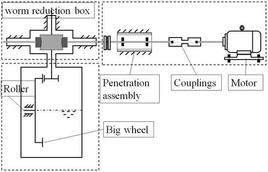
Figure 1. The relevant components of the industrial reactor in this paper.

4. Materials and Methods

4.1. Problem Definition

Assume that there are C channels of sensor data, represented as follows:

$$X=(X^1,X^2,...,X^C)$$

where the data length of each channel is T, simulating a Ts-second data monitoring process. Thus, the i-th channel of X is expressed as $X^i={[X_1^i,X_2^i,...X_T^i]}^T$. To simulate scenarios of data missing and channel missing, we designed a masking matrix $M=(M^1,M^2,...,M^C)$, where M has the same shape as X. This study uses M to index whether the corresponding elements in X have missing data. The elements of M are defined as follows:

$$M_t^c=\left\{\begin{array}{cc}0& if{X}_t^{c}ismissing.\\ 1& if{X}_t^{c}isnotmissing.\end{array}\right.$$

(1)

Here, based on Equation (1), we use M to compute the data in cases where data missing occurs.

$${\tilde{X}}_t^c={(M\times X)}_t^c=\left\{\begin{array}{cc}{X}_t^c& if{M}_t^c=1.\\ 0& if{M}_t^c=0.\end{array}\right.$$

(2)

Figure 2 illustrates the process of simulating data missing in the data preprocessing stage of the imputation problem in this paper, where the original data are processed based on the masking matrix.

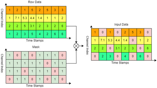
Figure 2. The schematic diagram for data simulation in the imputation problem.

In the subsequent experimental setup, we processed the data based on random data point missing and random channel missing scenarios. Specifically, in the random data point missing imputation task, the elements of M were randomly set to 0 with a certain proportion. In the random channel missing imputation task, one of the all channels in M was randomly set to 0. The objective of the experiment is to train and obtain an optimal mapping $f:\tilde{X}\to X$, such that the imputation error is minimized. The optimization objective is as follows:

$$\underset{f}{min}[M\times (\left|\right|f\left(\tilde{x}\right)-{x\left|\right|}_2^2\left)\right]$$

(3)

4.2. Proposed Method

The overall architecture of the DTM model proposed in this paper is shown in Figure 3. In current deep learning algorithms, Batch Normalization (BN) has been proven to be an effective preprocessing method that helps the model understand and extract features from time series data. In the data point imputation task, the masked data are also normalized using BN, and de-normalization is applied at the output layer to reconstruct the statistical features of the data. However, in the channel imputation task, data that are completely zero can introduce incorrect statistical information, so BN is not applied in this case.

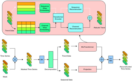
Figure 3. The architecture of the proposed method.

Additionally, this paper follows the time series decomposition approach, splitting the data into trend and seasonal components. On the one hand, the trend component, which occupies the dominant part of the time series, contains a significant amount of low-frequency data and is highly influenced by the coupling relationships between channels. On the other hand, the seasonal component contains less information and has a higher noise content, making it sensitive to channel variations and difficult to model effectively. Therefore, in capturing the coupling relationships between channels, this paper mainly focuses on the coupling information within the trend component.

For time series reconstruction, Zeng et al. (2023) [51] indicated that good data prediction performance can be achieved using only linear layers. Based on this, we input the features of the two components into independent linear layers for reconstruction, aiming to achieve high data modeling accuracy with relatively few operations. As a result, the reconstructed sequences contain the sequence information of their respective dimensions and, through a shared encoder, also capture deep information from the other dimension. In modeling the trend component, our proposed MixTransformer module not only performs data modeling at both the sequence and channel levels for the trend component but also captures and utilizes the coupling relationships between the two dimensions for data modeling.

4.2.1. Time Series Decomposite

For data preprocessing, Wu et al., 2021 [52] were the first to propose the use of time series decomposition in time series forecasting, and this has now become a common method in time series analysis. This approach enhances the predictability of the original data. This method applies a sliding average kernel to the input sequence to extract the trend component of the time series. The difference between the original sequence and the trend component is regarded as the seasonal component.

The formula for time series decomposition is as follows:

$$X_{trend,t}^c={\displaystyle \frac{1}{w}}\sum _{j=0}^w{\tilde{X}}_{t+j}^c$$

(4)

$$X_{seasonal,t}^c={\tilde{X}}_t^c-X_{trend,t}^c$$

(5)

where t represents the timestamp of X, and c represents the channel index of the sequence.

Building on the decomposition scheme, Zhou et al., 2022 [53] further proposed using a mixture of experts strategy. Its core idea is to combine the trend components extracted by moving average kernels with varying kernel sizes. The method adopted in this paper is based on the decomposition approach used in Autoformer to reduce computational overhead. Figure 4 illustrates the time series decomposition process, while Figure 5 shows the corresponding spectrum. The original data represent a sine function with added Gaussian white noise following $\mathcal{N}(0,0.2)$. The “Trend data” denotes the trend sequence obtained after decomposition, and the “Seasonal data” represents the local sequence.

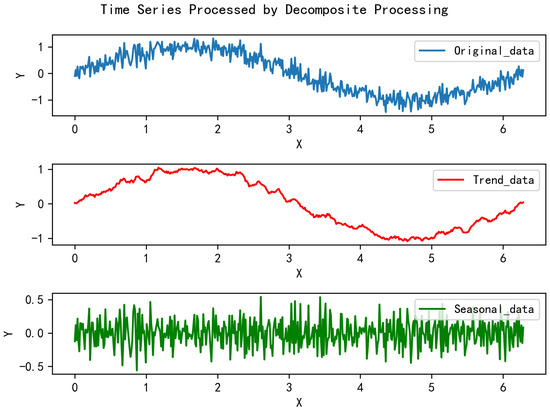
Figure 4. The diagram of the time series decomposition process.

Figure 5. The spectrum diagram of the decomposition process.

Figure 6 illustrates the denoising results of the temporal decomposition module on a sinusoidal function under varying noise levels. To visually demonstrate the denoising performance, we assume all noise to be additive white Gaussian noise with zero mean, where different variances correspond to distinct noise intensities. By comparing the mean square error (MSE) between the trend component output by the temporal decomposition module and the original noise-free sequence, it is evident that the time series decomposition method effectively suppresses additive white Gaussian noise. Specifically, the MSE values remain significantly lower across all tested noise levels, demonstrating the method’s robustness in preserving the intrinsic signal structure while isolating stochastic noise components.

Figure 6. The influence of AWGN on time series decomposition.

From Figure 4 and Figure 5, it can be observed that the “Trend data” preserves the overall trend of the original sequence, which includes the majority of the low-frequency components. On the other hand, the “Seasonal data” reflects the short-term variations of the sequence, primarily capturing the high-frequency components. This part of the data has a relatively low amplitude and contains less critical information from the original sequence. Therefore, it indicates that the focus of our time series imputation task should be on the “Trend data”.

Figure 7 depicts the Pearson correlation coefficients between Seasonal Data, Trend Data, and Original Data under the same conditions as in Figure 6. As the noise variance increases, the correlation between the Trend data and the Noised data gradually decreases, indicating that the proportion of the data information captured by the Trend component decreases. Conversely, the correlation coefficient for Seasonal Data increases, suggesting that the Seasonal component retains a growing share of the information. Furthermore, the correlation coefficients between Seasonal and Trend remain consistently low, demonstrating that the two components are approximately orthogonal. These observations illustrate that the time series decomposition method effectively separates the data into two uncorrelated components while minimizing information loss.

Figure 7. The influence of AWGN on the correlation between different portions.

4.2.2. MixTransformer

To enable the model to fully capture the inter-channel correlations and sequential variations of the trend components in time series data, we propose the MixTransformer module, whose main architecture is shown in Figure 3. Trend data are embedded into the feature space separately along the channel dimension and the sequence dimension through word embedding. These features are further extracted using a shared encoder. Additionally, the shared encoder leverages internal vectors to achieve indirect coupling and interaction between inter-channel and sequential information, thereby capturing the complex features of time series data. The extracted features are subsequently processed by a projection layer for sequence reconstruction, completing the reconstruction of the original trend sequence information.

For positional encoding along the sequence dimension, we adopt the encoding method used in Transformer models. For the input sequence $X\in R^{T\times C}$, after undergoing time series decomposition processing, we obtain $X_{trend}\in R^{T\times C}$ and $X_{seasonal}\in R^{T\times C}$ with unchanged shapes. Here, $X_{trend}$ is calculated through a 1D convolutional layer and Formula (7), respectively, to embed the channel dimension, resulting in $Em{b}_{trend}\in R^{T\times D_{model}}$ as Formula (6).

$$Em{b}_{trend}=Con{v}_{1D}\left(X_{trend}\right)+Pos\left(X_{trend}\right)$$

(6)

Here, $Con{v}_{1D}\left(\right)$ represents a 1D convolution applied to the last dimension of $X_{trend}$, and $Pos\left(\right)$ denotes Position Embedding, whose encoding value for time step t is defined by Equation (7).

$$P_t^i=f{\left(t\right)}^i:=\left\{\begin{array}{cc}sin(w_k·t)& ifi=2k\\ cos(w_k·t)& ifi=2k+1\end{array}\right.$$

(7)

where

$$w_k={\displaystyle \frac{1}{10,{000}^{2k/d}}}$$

We transposed the $X_{trend}$ and performed the same operations to obtain positional encoding along the channel dimension. The encoded sequence, after convolutional processing to extract the corresponding dimensional features, incorporates sequence information through positional encoding. Here, we employed two different 1D convolutional layers to encode both the temporal and channel dimensions to transform the time series into tokens for input to the Transformer, while ensuring that the data can be encoded independently across channels in the temporal dimension and independently across time in the channel dimension. Therefore, we obtain the data embedding $Em{b}_{trend}^{\prime }\in R^{C\times D_{model}}$ corresponding to the transpose of $X_{trend}$.

In traditional Transformer-based models, single-dimensional sequences are directly used for downstream tasks or reconstructed in an encoder–decoder architecture after encoding. These methods lack the computation of coupled information across multiple dimensions, leading to suboptimal performance.

To address this issue, we utilized a shared encoder for data encoding. According to the attention computation Formula (8), during the calculation of self-attention or multi-head attention, $W_Q$, $W_K$, and $W_V$ are trained to learn feature representations corresponding to the input vectors. Therefore, for sequence-wise embedding vectors and channel-wise embedding vectors, the shared encoder weights $W_Q$, $W_K$, and $W_V$ enable indirect interactions between the two dimensions. This ensures that deep-level coupling information can be extracted without losing the original embedding information, thereby enhancing the sequence construction process.

$$Attention(Q,K,V)=softmax({\displaystyle \frac{Q{K}^T}{\sqrt{d_k}}})V$$

(8)

where $Q=W_{Q}X, V=W_{V}X, K=W_{K}X$. $W_Q, W_K, W_V$ are learnable parameters. We employed the Transformer module as the shared encoder. Based on the aforementioned analysis, the embedding data from the temporal dimension and the channel dimension can achieve indirect interaction during the training process. Through the shared encoder, we obtain the vectors $En{c}_{Channel}\in R^{T\times D_{model}}$ and $En{c}_{Temporal}\in R^{C\times D_{model}}$, which are mapped into the encoding space for both the channel and temporal dimensions.

Finally, the vectors encoded by the shared encoder are processed through separate linear layers to reconstruct the original trend sequence along the temporal and channel dimensions. The methods for sequence reconstruction and channel reconstruction are described in Formulas (9) and (10), respectively. These reconstructed components are then summed to obtain the final reconstructed trend sequence. Thus, the reconstructed trend data are calculated by Formula (11). Following the principles outlined in the DLinear paper, linear layers are sufficient for sequence construction tasks while significantly reducing computational overhead. Algorithm 1 demonstrates the detailed training process of the proposed DTM model.

$$X_{seq}={(En{c}_{Temporal}{W}_{seq}+b_{seq})}^{\prime }$$

(9)

$$X_c=En{c}_{Channel}{W}_c+b_c$$

(10)

$$Rec\_X_{trend}=X_{seq}+X_c$$

(11)

where $X_{seq}\in R^{T\times C}$, $X_c\in R^{T\times C}$, $W_{seq}\in R^{D_{model}\times T}$, $W_c\in R^{D_{model}\times C}$, $b_{seq}\in R^{C\times T}$, $b_c\in R^{T\times C}$, symbol′ means Transpose process.

Algorithm 1 Training Process of DTM

Require: Time-series data X, mask matrix M, batch size B, learning rate $\eta$, number of epochs E Ensure: Trained DTM model parameters $\theta$    1: Initialize the model parameters $\theta$ of DTM    2: for epoch $e=1,2,\dots ,E$ do    3:    Shuffle the training dataset $(X,M)$    4:    for each batch $(X_b,M_b)$ in $(X,M)$ do    5:      Apply the mask $M_b$ to the data $X_b$ to simulate missing data, producing ${\tilde{X}}_b$    6:      Perform data preprocessing:    7:           Normalize ${\tilde{X}}_b$ if required    8:           Decompose ${\tilde{X}}_b$ into trend and seasonal components using temporal decomposition    9:      Reconstruct the decomposed trend components using the MixTransformer module:  10:           Perform embedding in both sequence and channel dimensions  11:           Pass embeddings through the shared encoder to extract features  12:           Decode the features using linear layers to reconstruct the sequence and channel dimensions  13:      Reconstruct the seasonal components using the projection layer  14:      Combine reconstructed components to obtain the interpolated output ${\widehat{Y}}_b$  15:      Compute the loss $\mathcal{L}$ using the MSE loss function.  16:      Backpropagate the loss $\mathcal{L}$ to update model parameters $\theta$ using gradient descent with learning rate $\eta$  17:    end for  18: end for  19: return Trained DTM model parameters $\theta$

4.3. Comparative Discussion with Existing Models

Compared to models such as Transformer and Autoformer, DTM addresses the limitation of handling only channel-independent time series by performing separate feature extraction along the temporal and channel dimensions, while Transformer-based architectures primarily rely on self-attention mechanisms for global temporal dependencies, they inherently treat multi-channel data as isolated sequences, neglecting critical inter-channel correlations. In contrast, DTM explicitly decouples temporal dynamics and channel-wise interactions through dual-path encoding, enabling effective modeling of strongly coupled sensor data prevalent in industrial scenarios. When compared to CNN-based models like MICN and TCN, DTM overcomes the suboptimal performance caused by limited receptive fields through decomposition modules and Transformer modules.

To the best of our knowledge, the model most similar related to DTM is Crossformer. Both models utilize data from both temporal and channel dimensions to capture latent information in MTS. However, Crossformer employs a patch-based DSW embedding for encoding, whereas DTM adopts a CNN-based embedding approach. This distinction arises because DTM targets interpolation tasks, requiring point-to-point or point-to-segment feature extraction, while Crossformer focuses on prediction tasks, emphasizing segment-to-segment data interaction.

Additionally, Crossformer uses Two-Stage Attention (TSA) layer to process temporal and channel dimensions sequentially in a serial manner. In contrast, DTM’s MixTransformer computes temporal and channel dimensions in parallel. Consequently, the method proposed in this work exhibits significant distinctions from existing approaches in both architecture design and task-specific optimization.

4.4. Time Complexity Discussion

The analysis of our approach on time complexity is described below. We assumed that the input sequence length is L, the embedding dimension is $d_{model}$, and the number of encoder layers is $n_l$. Then: For the time series decomposition component, the time complexity is $O\left(L\right)$. For the temporal embedding component, which employs a Convolutional Neural Network (CNN)-based approach, the time complexity across both the sequence and channel dimensions is $O(L·k·C·d_{model})$. For the shared encoder, following Transformer’s method, the time complexity is $O(L·L·n_l)$. For the projection layer, the time complexity is $O(L·d_{model})$. Thus, the overall time complexity of DTM is: $O(L·(n_l·L+1+(k·C+1)·d_{model}))$.

5. Results

5.1. Overview of Data

The data used in the experiment were all collected from the constructed engineering prototype of the industrial reactor. These datasets include operational signals such as eddy current displacement, vibration, motor torque, and motor position obtained during 480 h of simulated operation of the prototype, enabling monitoring of the operating status of key components of the device. For the purposes of this study, it is assumed that only the eddy current displacement data, wheel motor torque, and wheel torque meter torque among the monitored data may encounter issues of data loss or channel loss. All the data used in the experiment were resampled to a frequency of 20 Hz.

Table 1 lists the sensor variables used, where the subscript numbers in the variables indicate sensors of the same type installed at different locations. Reference [54] indicates that heatmaps can visualize the correlations among multiple datasets; therefore, this study also employs heatmaps to represent the interrelationships among multi-channel data. Figure 8 is presented as a heat map to visualize the Pearson correlation coefficients between channels, demonstrating their coupling characteristics. The colors in the figure represent Pearson’s correlations between different variables within the range of −1 to +1: lighter shades near zero indicate no significant relationship between variables, while darker shades approaching 1 signify strong correlations. Darker red hues indicate stronger positive correlations between variables, whereas darker blue hues denote stronger negative correlations. The symbols on the X and Y axes correspond to different channel names. This heat map visually demonstrates the interaction relationships among the channel data in the dataset used.

Table 1. The sensor variable used in this article.

Physical Meanings of Variables	Variables
Torque of Rotary motor	A
Torque of wheel torque meter	T
Eddy current of large wheel surface gear	$I_1$, $I_2$, $I_3$

Figure 8. The correlation coefficient between channels.

5.2. Experimental Setup

To simulate the data missing scenarios encountered in real-world situations, we applied random masking to data points and channels from the experimental prototype data to represent two types of anomalies: missing data records and sensor failures. Specifically, data point masking was conducted with proportions of 10% and 25%, while sensor failures were represented by random single-channel masking. Each batch of input data had a batch size of 128, a sequence length of 100, and 5 data channels. The proposed model used the Mean Square Error (MSE) as the loss function, and the final evaluation metrics included both MSE, $R^2$ and Mean Absolute Error (MAE). The experiments were conducted on an RTX 4060 Ti GPU. To fully reflect the performance of time series imputation, the evaluation metrics selected for this study were MSE, MAE, and $R^2$. Lower MSE and MAE values indicate better model performance, while an $R^2$ value closer to 1 reflects a stronger model fit. The formulas for those evaluation metrics are shown below:

$$MAE=\mathbb{E}(\sum _{c=1}^C\sum _{t=1}^{T}M\times |X_t^c-f{(\tilde{x})}_t^c|)$$

(12)

$$MSE=\mathbb{E}(\sum _{c=1}^C\sum _{t=1}^{T}M\times ||X_t^c-f{(\tilde{x})}_t^c|{|}_2^2)$$

(13)

$$R^2=1-{\displaystyle \frac{{\sum }_{c=1}^C{\sum }_{t=1}^{T}M\times \left|\right|X_t^c-f{\left(\tilde{x}\right)}_t^c{\left|\right|}_2^2}{{\sum }_{c=1}^C{\sum }_{t=1}^{T}M\times \left|\right|X_t^c-\overline{X_t^c}{\left|\right|}_2^2}}$$

(14)

Since we aim to demonstrate that our proposed model exhibits sufficient stability and superiority compared to various types of models in the proposed numerical imputation tasks, we conducted extensive comparisons with a wide range of advanced models including CNN-based Model: MICN (2023) [55], TCN (2018) [56]; MLP-based Model: DLinear (2022) [51] and LightTS (2023) [57]; Transformer-based Model: Reformer (2020) [58], Informer (2021) [59], Pyraformer (2022) [60], Autoformer (2021) [61], FEDformer (2022) [53], Transformer (2017) [62], Crossformer (2023) [63], iTransformer(2023) [64] and ETSformer (2022) [65]; Other advanced Model TimesNet (2023) [66] and FiLM (2022) [67]. Overall, a total of 15 models are included for a comprehensive comparison.

5.3. Experimental Result

As described in Section 4.1, we designed three different imputation experiments. To enable a horizontal comparison, we also employed several state-of-the-art time series models for the same experimental tasks. The hyperparameters of each model were carefully adjusted to ensure optimal results. After multiple rounds of experiments, the results of DTM and the other models are presented in Table 1, Table 2, Table 3 and Table 4.

Table 2. The experimental results of masking rate is 10%.

Model	MSE	MAE	${\mathit{R}}^2$
Dlinear	0.1853	0.1769	0.8151
TCN *	0.4381	0.3505	0.5622
TimesNet	0.1487	0.1573	0.8516
Transformer † ⋄	0.2647	0.2268	0.7367
Autoformer †	0.4684	0.4709	0.5314
Crossformer †	0.2588	0.2280	0.7412
ETSformer †	0.2411	0.2211	0.7593
FEDformer †	0.1907	0.2053	0.8095
FiLM	0.1852	0.1777	0.8134
Informer †	0.2722	0.2339	0.7254
iTransformer †	0.1871	0.1790	0.8131
LightTS	0.2030	0.1920	0.7974
MICN *	0.1532	0.1678	0.8470
Pyraformer †	0.2175	0.2146	0.7927
Reformer †	0.2404	0.2150	0.7572
DTM	0.1765	0.1712	0.8237

* CNN based model; † Transformer based model; ⋄ Baseline model.

Table 3. The experimental results of masking rate is 25%.

Model	MSE	MAE	${\mathit{R}}^2$
Dlinear	0.2045	0.1907	0.7956
TCN *	0.4677	0.3523	0.5325
TimesNet	0.1605	0.1678	0.8397
Transformer † ⋄	0.2816	0.2367	0.7198
Autoformer †	0.4404	0.4288	0.5597
Crossformer †	0.2700	0.2335	0.7303
ETSformer †	0.2824	0.2407	0.7177
FEDformer †	0.2139	0.2148	0.7863
FiLM	0.2054	0.1917	0.7941
Informer †	0.2991	0.2473	0.6985
iTransformer †	0.2035	0.1909	0.7966
LightTS	0.2085	0.1940	0.7915
MICN *	0.1867	0.1995	0.8136
Pyraformer †	0.2263	0.2344	0.7739
Reformer †	0.2592	0.2307	0.7380
DTM	0.1905	0.1815	0.8097

* CNN based model; † Transformer based model; ⋄ Baseline model.

Table 4. The experimental results of randomly masking one channel.

Model	MSE	MAE	${\mathit{R}}^2$
Dlinear	0.9897	0.5398	−0.0002
TCN *	0.5790	0.4510	0.4051
TimesNet	0.9483	0.5193	0.0395
Transformer † ⋄	0.6151	0.4457	0.3939
Autoformer †	1.0856	0.5948	−0.0522
Crossformer †	0.6170	0.4870	0.4042
ETSformer †	0.4800	0.4317	0.5134
FEDformer †	0.8616	0.5130	0.1232
FiLM	0.9603	0.5302	−0.0001
Informer †	0.5019	0.4324	0.4914
iTransformer †	0.8834	0.4992	0.0657
LightTS	0.6264	0.4583	0.3701
MICN *	0.8026	0.5352	0.2164
Pyraformer †	0.5071	0.3840	0.5339
Reformer †	0.4773	0.3886	0.5079
DTM	0.4748	0.4031	0.5504

* CNN based model; † Transformer based model; ⋄ Baseline model.

To demonstrate the model’s performance on the interpolation task under varying missing data ratios, we conducted additional experiments with missing ratios of 40%, 50%, and 60%, and compared the results with those of the Pyraformer and Reformer models. The experimental results are presented in Figure 9.

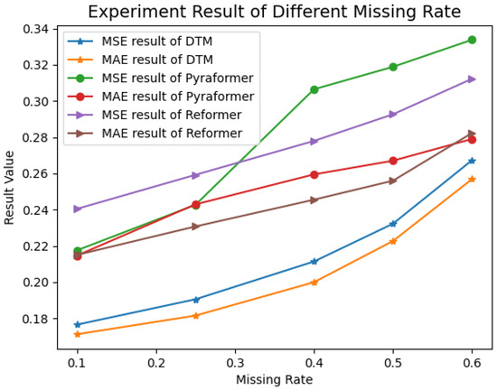
Figure 9. The experimental results under different missing rates.

5.4. Impact of Inter-Channel Correlations on DTM

In this section, we investigate how inter-channel correlation levels affect DTM. We designed the following comparative experiments: First, we selected five channels with low Pearson correlation coefficients from the Weather (https://www.bgc-jena.mpg.de/wetter/, accessed on 10 May 2025) dataset, as illustrated in Figure 10. Additionally, we chose six extra channels that exhibited high correlation coefficients with the aforementioned five channels, as shown in Figure 11. Subsequently, we employed DTM to conduct two sets of interpolation tasks: (1) Low-correlation scenario: Experiments using only the five low-correlation channels. (2) Coupled multi-channel scenario: Experiments using the combined data of all 11 channels, but focusing solely on imputation the original 5 low-correlation channels.

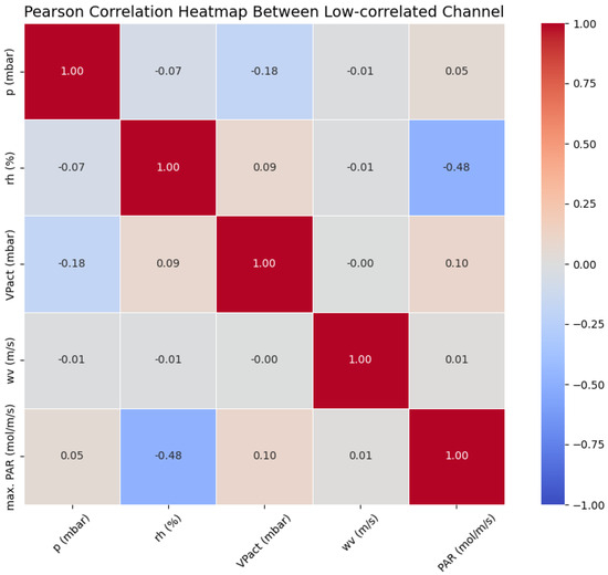
Figure 10. The heat map of low-correlated channel.

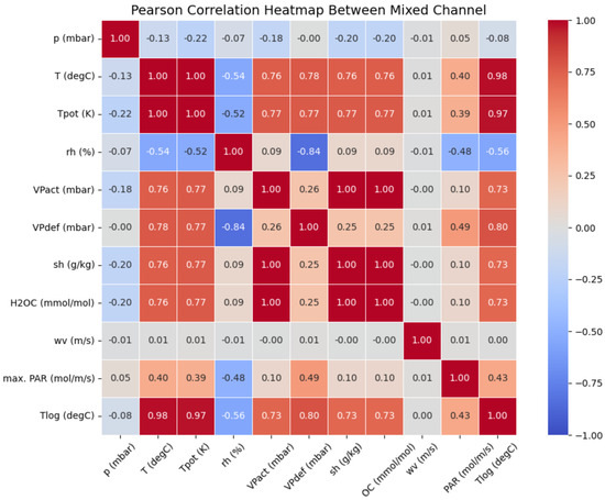
Figure 11. The heat map of the mixed channel.

The final experimental results are presented in Table 5, validating the advantages of incorporating multi-channel coupling information.

Table 5. The experimental result of different correlated data on DTM.

Metrics	10%, 5-5	25%, 5-5	Single, 5-5	10%, 11-5	25%, 11-5	Single, 11-5
MSE	0.2963	0.3161	1.4684	0.0535 ↓	0.0807 ↓	0.1910 ↓
MAE	0.3236	0.3427	0.9430	0.1463 ↓	0.1691 ↓	0.2983 ↓

X%, A-B means experiment with masking rate = X%, using A Channels data to imputation B Channels, single means randomly masking one channel, symbol ↓ denotes the a lower evaluation function value under the same masking strategy.

6. Discussion

We evaluated the proposed model and several state-of-the-art models on the same imputation tasks. The training performance comparison metrics used in the experiments were Mean Square Error (MSE), Mean Absolute Error (MAE), and $R^2$. The final experimental results are shown in Table 2, Table 3 and Table 4. Based on the experimental data, our proposed model consistently achieved the leading performance under various conditions, successfully meeting the target objectives of the tasks.

Compared to Transformer-based models, our proposed model outperformed the best-performing Reformer model in the channel-level imputation task, reducing the MSE by 0.0028. In the random data imputation task, our model also surpassed the best-performing iTransformer, achieving at least a 0.01 reduction in MSE. As shown in Figure 9, we observe that across data missing rates ranging from 0.1 to 0.6, both the MSE and MAE of DTM remain consistently lower than those of Reformer and Pyraformer, demonstrating the stable performance superiority of our proposed model.

Compared to the non-Transformer-based and CNN-based methods, such as TimesNet, its performance in scenarios with 10% and 25% masking rates surpasses DTM, demonstrating TimesNet’s robust sequence reconstruction capabilities. However, its performance significantly deteriorates in the random channel masking task. We also identified several models with performance deterioration patterns similar to TimesNet. Their $R^2$ values approach or even fall below 0, indicating that the imputation capability of these models is statistically comparable to naive mean-based imputation within the corresponding channel. This is likely because random value masking causes minimal disruption to the statistical information of individual channels, whereas the random channel masking task completely eliminates the statistical information of entire channels, presenting a substantial challenge for models equipped with sequence modeling capabilities. In contrast, DTM consistently ranks among the top-performing models across all three tasks in terms of R² values, demonstrating its robustness in effectively overcoming these challenges.

When compared to non-Transformer models such as DLinear and TCN, our proposed model exceeded their performance in at least one or more tasks. Even in tasks where it did not outperform these models, it maintained a comparable level of performance, demonstrating that our model is better suited to adapt to complex fault scenarios.

According to Figure 10 and Figure 11, we can observe that after adding six new channels, nearly all channels now possess corresponding highly correlated channels that reflect their coupling relationships. The experimental results in Table 5 demonstrate that the model performance shows significant improvement after channel augmentation. This indicates that our model performs poorly when handling data with low correlation relationships, while the introduction of coupling-enhanced channels substantially enhances its capability. These findings verify our model’s ability to achieve data interpolation through latent coupling relationships.

7. Conclusions

We summarize as follows: In the random data missing and random channel missing imputation tasks for sensor data in the industrial reactor, the DTM model proved to be a robust solution for completing the tasks. Among the three imputation tasks, DTM achieved leading performance in one task and ranked third in the other two. Our proposed model, DTM, integrates channel decoupling with sequence modeling, enhancing the model’s ability to capture multidimensional coupling relationships in multichannel data. Compared to the baseline model, DTM demonstrated improvements across multiple experimental metrics in various tasks. Specifically, MSE and MAE were reduced by up to 33.3% and 24.5%, respectively, while the R² value increased by a maximum of 39.73%, highlighting its statistical superiority. Experimental results demonstrate that DTM outperforms most Transformer-based and CNN-based algorithms in the imputation scenarios proposed in this paper.

References

- Qi, B.; Liang, J.; Tong, J. Fault diagnosis techniques for nuclear power plants: A review from the artificial intelligence perspective. Energies 2023, 16, 1850. [Google Scholar] [CrossRef]
- Tonday Rodriguez, J.C.; Perry, D.; Rahman, M.A.; Alam, S.B. An Intelligent Hierarchical Framework for Efficient Fault Detection and Diagnosis in Nuclear Power Plants. In Proceedings of the Sixth Workshop on CPS&IoT Security and Privacy, Salt Lake City, UT, USA, 14–18 October 2024; pp. 80–92. [Google Scholar]
- Kozma, R.; Nabeshima, K. Studies on the detection of incipient coolant boiling in nuclear reactors using artificial neural networks. Ann. Nucl. Energy 1995, 22, 483–496. [Google Scholar] [CrossRef]
- Nabeshima, K.; Suzudo, T.; Suzuki, K.; Türkcan, E. Real-time nuclear power plant monitoring with neural network. J. Nucl. Sci. Technol. 1998, 35, 93–100. [Google Scholar] [CrossRef]
- Nabeshima, K.; Suzudo, T.; Seker, S.; Ayaz, E.; Barutcu, B.; Türkcan, E.; Ohno, T.; Kudo, K. On-line neuro-expert monitoring system for borssele nuclear power plant. Prog. Nucl. Energy 2003, 43, 397–404. [Google Scholar] [CrossRef]
- Lee, C.K.; Chang, S.J. Fault detection in multi-core C&I cable via machine learning based time-frequency domain reflectometry. Appl. Sci. 2019, 10, 158. [Google Scholar]
- Mandal, S.; Santhi, B.; Sridhar, S.; Vinolia, K.; Swaminathan, P. Nuclear power plant thermocouple sensor-fault detection and classification using deep learning and generalized likelihood ratio test. IEEE Trans. Nucl. Sci. 2017, 64, 1526–1534. [Google Scholar] [CrossRef]
- Peng, B.S.; Xia, H.; Liu, Y.K.; Yang, B.; Guo, D.; Zhu, S.M. Research on intelligent fault diagnosis method for nuclear power plant based on correlation analysis and deep belief network. Prog. Nucl. Energy 2018, 108, 419–427. [Google Scholar] [CrossRef]
- Bang, S.S.; Shin, Y.J. Classification of faults in multicore cable via time–frequency domain reflectometry. IEEE Trans. Ind. Electron. 2019, 67, 4163–4171. [Google Scholar] [CrossRef]
- Saeed, H.A.; Wang, H.; Peng, M.; Hussain, A.; Nawaz, A. Online fault monitoring based on deep neural network & sliding window technique. Prog. Nucl. Energy 2020, 121, 103236. [Google Scholar]
- Abdelghafar, S.; El-shafeiy, E.; Mohammed, K.K.; Drawish, A.; Hassanien, A.E. CNN-Based Fault Detection in Nuclear Power Reactors Using Real-Time Sensor Data. In Business Intelligence and Information Technology; Proceedings of BIIT 2023; Springer: Berlin/Heidelberg, Germany, 2023; pp. 639–649. [Google Scholar]
- Yang, J.; Kim, J. An accident diagnosis algorithm using long short-term memory. Nucl. Eng. Technol. 2018, 50, 582–588. [Google Scholar] [CrossRef]
- Choi, J.; Lee, S.J. Consistency index-based sensor fault detection system for nuclear power plant emergency situations using an LSTM network. Sensors 2020, 20, 1651. [Google Scholar] [CrossRef]
- Yang, J.; Kim, J. Accident diagnosis algorithm with untrained accident identification during power-increasing operation. Reliab. Eng. Syst. Saf. 2020, 202, 107032. [Google Scholar] [CrossRef]
- Zhou, G.; Zheng, S.; Yang, S.; Yi, S. A Novel Transformer-Based Anomaly Detection Model for the Reactor Coolant Pump in Nuclear Power Plants. Sci. Technol. Nucl. Install. 2024, 2024, 9455897. [Google Scholar] [CrossRef]
- Yi, S.; Zheng, S.; Yang, S.; Zhou, G.; He, J. Robust transformer-based anomaly detection for nuclear power data using maximum correntropy criterion. Nucl. Eng. Technol. 2024, 56, 1284–1295. [Google Scholar] [CrossRef]
- Shen, B.; Yao, L.; Ge, Z. Nonlinear probabilistic latent variable regression models for soft sensor application: From shallow to deep structure. Control Eng. Pract. 2020, 94, 104198. [Google Scholar] [CrossRef]
- Yuan, X.; Huang, B.; Wang, Y.; Yang, C.; Gui, W. Deep learning-based feature representation and its application for soft sensor modeling with variable-wise weighted SAE. IEEE Trans. Ind. Inform. 2018, 14, 3235–3243. [Google Scholar] [CrossRef]
- Wang, X.; Liu, H. Data supplement for a soft sensor using a new generative model based on a variational autoencoder and Wasserstein GAN. J. Process Control 2020, 85, 91–99. [Google Scholar] [CrossRef]
- Yao, L.; Ge, Z. Deep learning of semisupervised process data with hierarchical extreme learning machine and soft sensor application. IEEE Trans. Ind. Electron. 2017, 65, 1490–1498. [Google Scholar] [CrossRef]
- Horn, Z.; Auret, L.; McCoy, J.; Aldrich, C.; Herbst, B. Performance of convolutional neural networks for feature extraction in froth flotation sensing. IFAC-PapersOnLine 2017, 50, 13–18. [Google Scholar] [CrossRef]
- Yuan, X.; Qi, S.; Shardt, Y.A.; Wang, Y.; Yang, C.; Gui, W. Soft sensor model for dynamic processes based on multichannel convolutional neural network. Chemom. Intell. Lab. Syst. 2020, 203, 104050. [Google Scholar] [CrossRef]
- Wei, J.; Guo, L.; Xu, X.; Yan, G. Soft sensor modeling of mill level based on convolutional neural network. In Proceedings of the The 27th Chinese Control and Decision Conference (2015 CCDC), Qingdao, China, 23–25 May 2015; pp. 4738–4743. [Google Scholar]
- Ke, W.; Huang, D.; Yang, F.; Jiang, Y. Soft sensor development and applications based on LSTM in deep neural networks. In Proceedings of the 2017 IEEE Symposium Series on Computational Intelligence (SSCI), Honolulu, HI, USA, 27 November–1 December 2017; pp. 1–6. [Google Scholar]
- Yuan, X.; Li, L.; Wang, Y. Nonlinear dynamic soft sensor modeling with supervised long short-term memory network. IEEE Trans. Ind. Informatics 2019, 16, 3168–3176. [Google Scholar] [CrossRef]
- Raghavan, S.V.; Radhakrishnan, T.; Srinivasan, K. Soft sensor based composition estimation and controller design for an ideal reactive distillation column. ISA Trans. 2011, 50, 61–70. [Google Scholar] [CrossRef]
- Yin, X.; Niu, Z.; He, Z.; Li, Z.S.; Lee, D.h. Ensemble deep learning based semi-supervised soft sensor modeling method and its application on quality prediction for coal preparation process. Adv. Eng. Inform. 2020, 46, 101136. [Google Scholar] [CrossRef]
- Andridge, R.R.; Little, R.J. A review of hot deck imputation for survey non-response. Int. Stat. Rev. 2010, 78, 40–64. [Google Scholar] [CrossRef]
- Van Buuren, S. Multiple imputation of discrete and continuous data by fully conditional specification. Stat. Methods Med. Res. 2007, 16, 219–242. [Google Scholar] [CrossRef]
- Pujianto, U.; Wibawa, A.P.; Akbar, M.I. K-nearest neighbor (k-NN) based missing data imputation. In Proceedings of the 2019 5th International Conference on Science in Information Technology (ICSITech), Yogyakarta, Indonesia, 23–24 October 2019; pp. 83–88. [Google Scholar]
- Troyanskaya, O.; Cantor, M.; Sherlock, G.; Brown, P.; Hastie, T.; Tibshirani, R.; Botstein, D.; Altman, R.B. Missing value estimation methods for DNA microarrays. Bioinformatics 2001, 17, 520–525. [Google Scholar] [CrossRef]
- Stekhoven, D.J.; Bühlmann, P. MissForest—non-parametric missing value imputation for mixed-type data. Bioinformatics 2012, 28, 112–118. [Google Scholar] [CrossRef]
- Doreswamy, I.G.; Manjunatha, B. Performance evaluation of predictive models for missing data imputation in weather data. In Proceedings of the 2017 International Conference on Advances in Computing, Communications and Informatics (ICACCI), Udupi, India, 13–16 September 2017; pp. 1327–1334. [Google Scholar]
- Mallinson, H.; Gammerman, A. Imputation Using Support Vector Machines; Department of Computer Science Royal Holloway, University of London Egham: London, UK, 2003. [Google Scholar]
- Noor, T.H.; Almars, A.; Gad, I.; Atlam, E.S.; Elmezain, M. Spatial impressions monitoring during COVID-19 pandemic using machine learning techniques. Computers 2022, 11, 52. [Google Scholar] [CrossRef]
- Vincent, P.; Larochelle, H.; Bengio, Y.; Manzagol, P.A. Extracting and composing robust features with denoising autoencoders. In Proceedings of the 25th International Conference on Machine Learning, Helsinki, Finland, 5–9 July 2008; pp. 1096–1103. [Google Scholar]
- Li, J.; Ren, W.; Han, M. Variational auto-encoders based on the shift correction for imputation of specific missing in multivariate time series. Measurement 2021, 186, 110055. [Google Scholar] [CrossRef]
- Yoon, J.; Jordon, J.; Schaar, M. Gain: Missing data imputation using generative adversarial nets. In Proceedings of the International Conference on Machine Learning, Stockholm, Sweden, 10–15 July 2018; pp. 5689–5698. [Google Scholar]
- Qin, R.; Wang, Y. ImputeGAN: Generative adversarial network for multivariate time series imputation. Entropy 2023, 25, 137. [Google Scholar] [CrossRef]
- Khan, W.; Zaki, N.; Ahmad, A.; Masud, M.M.; Ali, L.; Ali, N.; Ahmed, L.A. Mixed data imputation using generative adversarial networks. IEEE Access 2022, 10, 124475–124490. [Google Scholar] [CrossRef]
- Yıldız, A.Y.; Koç, E.; Koç, A. Multivariate time series imputation with transformers. IEEE Signal Process. Lett. 2022, 29, 2517–2521. [Google Scholar] [CrossRef]
- Nie, T.; Qin, G.; Ma, W.; Mei, Y.; Sun, J. ImputeFormer: Low rankness-induced transformers for generalizable spatiotemporal imputation. In Proceedings of the 30th ACM SIGKDD Conference on Knowledge Discovery and Data Mining, Barcelona, Spain, 25–29 August 2024; pp. 2260–2271. [Google Scholar]
- Stellwagen, E.; Tashman, L. ARIMA: The Models of Box and Jenkins. Foresight Int. J. Appl. Forecast. 2013, 30, 28–33. [Google Scholar]
- Feng, J.; Li, Y.; Zhang, C.; Sun, F.; Meng, F.; Guo, A.; Jin, D. Deepmove: Predicting human mobility with attentional recurrent networks. In Proceedings of the 2018 World Wide Web Conference, Lyons, France, 23–27 April 2018; pp. 1459–1468. [Google Scholar]
- Qin, Y.; Song, D.; Cheng, H.; Cheng, W.; Jiang, G.; Cottrell, G.W. A dual-stage attention-based recurrent neural network for time series prediction. In Proceedings of the 26th International Joint Conference on Artificial Intelligence, Melbourne, Australia, 19–25 August 2017; pp. 2627–2633. [Google Scholar]
- Bai, L.; Yao, L.; Kanhere, S.S.; Wang, X.; Sheng, Q.Z. STG2Seq: Spatial-Temporal Graph to Sequence Model for Multi-step Passenger Demand Forecasting. In Proceedings of the Twenty-Eighth International Joint Conference on Artificial Intelligence, Macao, China, 10–16 August 2019; pp. 1981–1987. [Google Scholar] [CrossRef]
- Wu, Z.; Pan, S.; Long, G.; Jiang, J.; Chang, X.; Zhang, C. Connecting the dots: Multivariate time series forecasting with graph neural networks. In Proceedings of the 26th ACM SIGKDD International Conference on Knowledge Discovery & Data Mining, Virtual Event, CA, USA, 6–10 July 2020; pp. 753–763. [Google Scholar]
- Zhang, Z.; Meng, L.; Gu, Y. SageFormer: Series-Aware Framework for Long-Term Multivariate Time-Series Forecasting. IEEE Internet Things J. 2024, 11, 18435–18448. [Google Scholar] [CrossRef]
- He, H.; Zhang, Q.; Wang, S.; Yi, K.; Niu, Z.; Cao, L. Learning Informative Representation for Fairness-Aware Multivariate Time-Series Forecasting: A Group-Based Perspective. IEEE Trans. Knowl. Data Eng. 2024, 36, 2504–2516. [Google Scholar] [CrossRef]
- Wang, C.; Wang, H.; Zhang, X.; Liu, Q.; Liu, M.; Xu, G. A Transformer-Based Industrial Time Series Prediction Model With Multivariate Dynamic Embedding. IEEE Trans. Ind. Inform. 2025, 21, 1813–1822. [Google Scholar] [CrossRef]
- Zeng, A.; Chen, M.; Zhang, L.; Xu, Q. Are transformers effective for time series forecasting? In Proceedings of the AAAI Conference on Artificial Intelligence, Washington, DC, USA, 7–14 February 2023; Volume 37, pp. 11121–11128. [Google Scholar]
- Wu, H.; Xu, J.; Wang, J.; Long, M. Autoformer: Decomposition Transformers with Auto-Correlation for Long-Term Series Forecasting. In Advances in Neural Information Processing Systems 34 (NeurIPS 2021); Ranzato, M., Beygelzimer, A., Dauphin, Y., Liang, P., Vaughan, J.W., Eds.; Curran Associates, Inc.: Red Hook, NY, USA, 2021; Volume 34, pp. 22419–22430. [Google Scholar]
- Zhou, T.; Ma, Z.; Wen, Q.; Wang, X.; Sun, L.; Jin, R. FEDformer: Frequency enhanced decomposed transformer for long-term series forecasting. In Proceedings of the 39th International Conference on Machine Learning (ICML 2022), Baltimore, MD, USA, 17–23 July 2022. [Google Scholar]
- Binali, R. Experimental and machine learning comparison for measurement the machinability of nickel based alloy in pursuit of sustainability. Measurement 2024, 236, 115142. [Google Scholar] [CrossRef]
- Wang, H.; Peng, J.; Huang, F.; Wang, J.; Chen, J.; Xiao, Y. MICN: Multi-scale Local and Global Context Modeling for Long-term Series Forecasting. In Proceedings of the 11th International Conference on Learning Representations, Kigali, Rwanda, 1–5 May 2023. [Google Scholar]
- Bai, S.; Kolter, J.Z.; Koltun, V. An Empirical Evaluation of Generic Convolutional and Recurrent Networks for Sequence Modeling. arXiv 2018, arXiv:1803.01271. [Google Scholar]
- Campos, D.; Zhang, M.; Yang, B.; Kieu, T.; Guo, C.; Jensen, C.S. LightTS: Lightweight Time Series Classification with Adaptive Ensemble Distillation. Proc. ACM Manag. Data 2023, 1, 171:1–171:27. [Google Scholar] [CrossRef]
- Kitaev, N.; Kaiser, L.; Levskaya, A. Reformer: The Efficient Transformer. In Proceedings of the International Conference on Learning Representations, Addis Ababa, Ethiopia, 26–30 April 2020. [Google Scholar]
- Zhou, H.; Zhang, S.; Peng, J.; Zhang, S.; Li, J.; Xiong, H.; Zhang, W. Informer: Beyond Efficient Transformer for Long Sequence Time-Series Forecasting. In Proceedings of the The Thirty-Fifth AAAI Conference on Artificial Intelligence, AAAI 2021, Virtual Conference, 2–9 February 2021; AAAI Press: Vancouver, BC, Canada, 2021; Volume 35, pp. 11106–11115. [Google Scholar]
- Liu, S.; Yu, H.; Liao, C.; Li, J.; Lin, W.; Liu, A.X.; Dustdar, S. Pyraformer: Low-Complexity Pyramidal Attention for Long-Range Time Series Modeling and Forecasting. In Proceedings of the International Conference on Learning Representations, Virtual Event, 25–29 April 2022. [Google Scholar]
- Wu, H.; Xu, J.; Wang, J.; Long, M. Autoformer: Decomposition Transformers with Auto-Correlation for Long-Term Series Forecasting. In Proceedings of the Advances in Neural Information Processing Systems, Virtual Event, 6–14 December 2021. [Google Scholar]
- Vaswani, A. Attention is all you need. In Advances in Neural Information Processing Systems 30; Curran Associates Inc.: Red Hook, NY, USA, 2017; ISBN 9781510860964. [Google Scholar]
- Zhang, Y.; Yan, J. Crossformer: Transformer Utilizing Cross-Dimension Dependency for Multivariate Time Series Forecasting. In Proceedings of the International Conference on Learning Representations, Kigali, Rwanda, 1–5 May 2023. [Google Scholar]
- Liu, Y.; Hu, T.; Zhang, H.; Wu, H.; Wang, S.; Ma, L.; Long, M. iTransformer: Inverted Transformers Are Effective for Time Series Forecasting. arXiv 2023, arXiv:2310.06625. [Google Scholar]
- Woo, G.; Liu, C.; Sahoo, D.; Kumar, A.; Hoi, S. Etsformer: Exponential smoothing transformers for time-series forecasting. arXiv 2022, arXiv:2202.01381. [Google Scholar]
- Wu, H.; Hu, T.; Liu, Y.; Zhou, H.; Wang, J.; Long, M. TimesNet: Temporal 2D-Variation Modeling for General Time Series Analysis. In Proceedings of the International Conference on Learning Representations, Kigali, Rwanda, 1–5 May 2023. [Google Scholar]
- Zhou, T.; Ma, Z.; Wen, Q.; Sun, L.; Yao, T.; Yin, W.; Jin, R. Film: Frequency improved legendre memory model for long-term time series forecasting. Adv. Neural Inf. Process. Syst. 2022, 35, 12677–12690. [Google Scholar]
Disclaimer/Publisher’s Note: The statements, opinions and data contained in all publications are solely those of the individual author(s) and contributor(s) and not of MDPI and/or the editor(s). MDPI and/or the editor(s) disclaim responsibility for any injury to people or property resulting from any ideas, methods, instructions or products referred to in the content. |
© 2025 by the authors. Licensee MDPI, Basel, Switzerland. This article is an open access article distributed under the terms and conditions of the Creative Commons Attribution (CC BY) license (https://creativecommons.org/licenses/by/4.0/).