Research on Intelligent Early Warning and Emergency Response Mechanism for Tunneling Face Gas Concentration Based on an Improved KAN-iTransformer

Abstract

The tunneling face poses a significant risk for gas disaster in coal mining due to the complex interplay of geological conditions, ventilation strategies, and construction techniques, resulting in nonlinear and spatiotemporal dynamics in gas concentration distribution. Accurate prediction of gas levels is crucial for ensuring the safety of coal mining operations. This study introduces a novel approach for gas concentration forecasting at the tunneling face by integrating the Kolmogorov–Arnold Network (KAN) with an enhanced iTransformer model, leveraging multi-source sensor data for enhanced predictive capabilities. KAN improves the feature extraction ability due to flexible mapping kernel function that is capable of capturing complicated nonlinearities between gas emission volume and environmental variables. iTransformer, with concentrated attention mechanism and sparsity pattern, can further model very long-term sequence dependencies and learn to capture multi-scale features. As a whole, they address the problem of gradient vanishing and insufficient feature extraction in the temporal sequential prediction models based on deep learning methods with long sequences input, leading to significant improvements in prediction accuracy and model stability. Experiments on site monitoring datasets demonstrate that the proposed KAN + iTransformer model achieved better fitting and generalization capacity than two baseline models (iTransformer, Transformer) for gas concentration prediction.

1. Introduction

Coal remains the dominant source of primary energy globally, despite significant advancements in clean energy. It is indispensable in power generation, metallurgy, and chemical engineering. However, as coal mining operations deepen and expand, safety concerns have escalated, particularly regarding gas-related incidents. Gas explosions and outbursts constitute over 70% of major coal mine accidents, leading to severe casualties and economic losses, hindering the coal industry’s progress. The tunneling face is especially prone to gas accumulation and unexpected emissions, with gas concentration changes being nonlinear, time-variant, and abrupt. Accurately predicting gas concentration at the tunneling face is a critical challenge in coal mine safety science.

Traditional methane concentration prediction methods can be categorized into two types: one involves statistical or machine learning approaches emphasizing interpretability and robustness; Bo et al. [1] employed a PSO–ELM hybrid prediction model to correlate geological factors with gas outbursts, enhancing the generalization capability of methane concentration forecasting. Chengmin et al. [2] analyzed the sensitivity of gas outburst parameters and the contribution ratio of gas sources, enabling methane concentration prediction in tunneling workfaces. Shenghao et al. [3] employed a hybrid machine learning model combining random forest and an improved corridor algorithm to screen factors influencing gas outburst volume, enabling methane concentration prediction. Weihua et al. [4] constructed a prediction model integrating LASSO feature selection, WOA parameter optimization, and XGBoost, significantly reducing the methane outburst prediction errors and providing an effective method for precise mine gas forecasting. Peng [5] et al. developed a high-precision gas outburst prediction model by integrating distribution estimation algorithms with an optimized immune genetic algorithm. Jun [6] et al. established a gas outburst prediction model based on gray prediction theory, utilizing multi-source data from multiple tunneling faces. Yongkang [7] et al. achieved critical gas outburst prediction by integrating an improved gray theory model with an RBF neural network.

Although such methods feature a straightforward modeling process and strong interpretability, they heavily rely on manual feature engineering and linear assumptions, making it difficult to capture the dynamic nonlinear relationships in gas outbursts. Moreover, these models are typically static, struggling to effectively capture the strong nonlinearity and abrupt changes in gas concentration that occur during tunneling operations.

Another category involves data-driven deep learning models for methane concentration prediction, emphasizing robust representation and modeling capabilities across temporal scales. Jingzhao et al. [8] proposed a hybrid GVSL prediction model integrating Genetic Algorithm-optimized Variational Modal Decomposition (GA-VMD) and Sparrow Search Algorithm-optimized Long Short-Term Memory Network (SSA-LSTM). This multi-algorithm collaborative optimization achieved temporal forecasting of methane outburst volumes in coal mining faces. Haifei et al. [9] constructed a coal mine gas outburst prediction model using RFECV feature selection and Bi-LSTM neural networks, achieving high-precision and reliable predictions for multi-factor time series. Liang et al. [10] proposed an Adamax-BiGRU model integrating the Adamax optimization algorithm, constructing a bidirectional GRU learning model for gas concentration time series using Adamax optimization. Li et al. [11] introduced a novel time series prediction model, MSA-BiLG, integrating a multi-scale attention mechanism with a BiLSTM-GRU neural architecture to enhance modeling capabilities between target variables and covariates. While such models can uncover nonlinear dependencies in time series data, they tend to lose critical historical information during long-sequence modeling, making it challenging to effectively capture the complex long-term spatiotemporal dependencies inherent in dynamic gas outburst processes.

With the rapid advancement of artificial intelligence in recent years, the field of time series forecasting has witnessed revolutionary progress. Transformers enable the direct computation of relationships between any two positions in a sequence through self-attention mechanisms. Many experts have leveraged Transformers to achieve long-term gas concentration forecasting. Yang et al. [12] proposed a multi-indicator early warning method integrating GF-KMeans intelligent threshold segmentation with the MOA-Transformer classification model. This approach significantly enhances early warning performance by optimizing both clustering centers and attention mechanisms. Qu et al. [13] proposed a methane concentration prediction model for coal mine tunnels based on the Improved Black Kite Algorithm (IBKA) and Informer-BiLSTM, enhancing the model’s efficiency and accuracy for long-term sequence predictions. Lai et al. [14] introduced a gas prediction method based on Enhanced Inverse Distance Weighted Interpolation with Informer (EIDW-Informer), strengthening the model’s long-term forecasting capabilities. Pan et al. [15] integrated genetic algorithms with Autoformer’s autocorrelation/decomposition framework to strengthen intrinsic correlations between covariates and target variables. All these studies treated sensor variables as random sets at each time step, failing to leverage the prior knowledge of sensors’ spatial layout within tunnels. This approach risks equal emphasis on physically unrelated distant sensors while underestimating strong dynamic coupling between adjacent sensors. Furthermore, concatenating all variables into tokens along the time dimension causes interference between different variables’ time series patterns. This obscures the causal relationships between specific variables driven by factors like ventilation networks and mining activities. The existing research primarily focuses on geological and ventilation parameters, neglecting the real-time impact of mining equipment operating parameters on gas desorption and emission dynamics.

Therefore, while existing models provide a valuable foundation, they fail to adequately address the unique challenges posed by the spatiotemporal coupling of tunneling faces, the coupling of equipment and environmental factors, and spatial topological constraints.

To address these challenges, this work focuses on multi-source sensor data from tunneling workfaces, constructing a methane concentration prediction model based on an improved KAN-iTransformer. On the data side, it incorporates noise reduction and anomaly handling tailored to underground data characteristics. On the model side, a time series Transformer serves as the backbone, integrated with graph attention to capture dynamic dependencies among sensors. A more interpretable functional approximation module (KAN) is introduced to enhance sample efficiency and stability. For prediction, a multi-step point–interval joint output and early warning strategy is proposed for safety threshold management, enabling early identification and quantitative assessment of threshold-exceeding risks. Compared with the baseline models, the proposed method demonstrates improvements in multi-step prediction accuracy, robustness, and early warning hit rate.

Our key innovations are as follows:

Architectural Level: We adopt the inverted tokenization approach of iTransformer, treating the entire historical sequence of each variable as a token. This enables the attention mechanism to operate at the variable dimension, explicitly learning dynamic dependencies among multi-source sensors.

Spatial Modeling: We replace standard self-attention with Graph Attention Networks (GAT). By constructing a graph structure based on sensor physical locations and ventilation networks, we inject spatial topology priors into the model, ensuring information aggregation aligns with the physical reality of underground tunnels.

Nonlinear Mapping: We replace traditional MLPs with Kolmogorov–Arnold Networks (KANs), whose learnable activation functions enable more flexible and precise approximations of the highly complex nonlinear relationships between gas outbursts and influencing factors. KANs demonstrate greater stability, particularly in regions with sparse data.

2. Project Background and Data Processing

2.1. Project Background and Data Sources

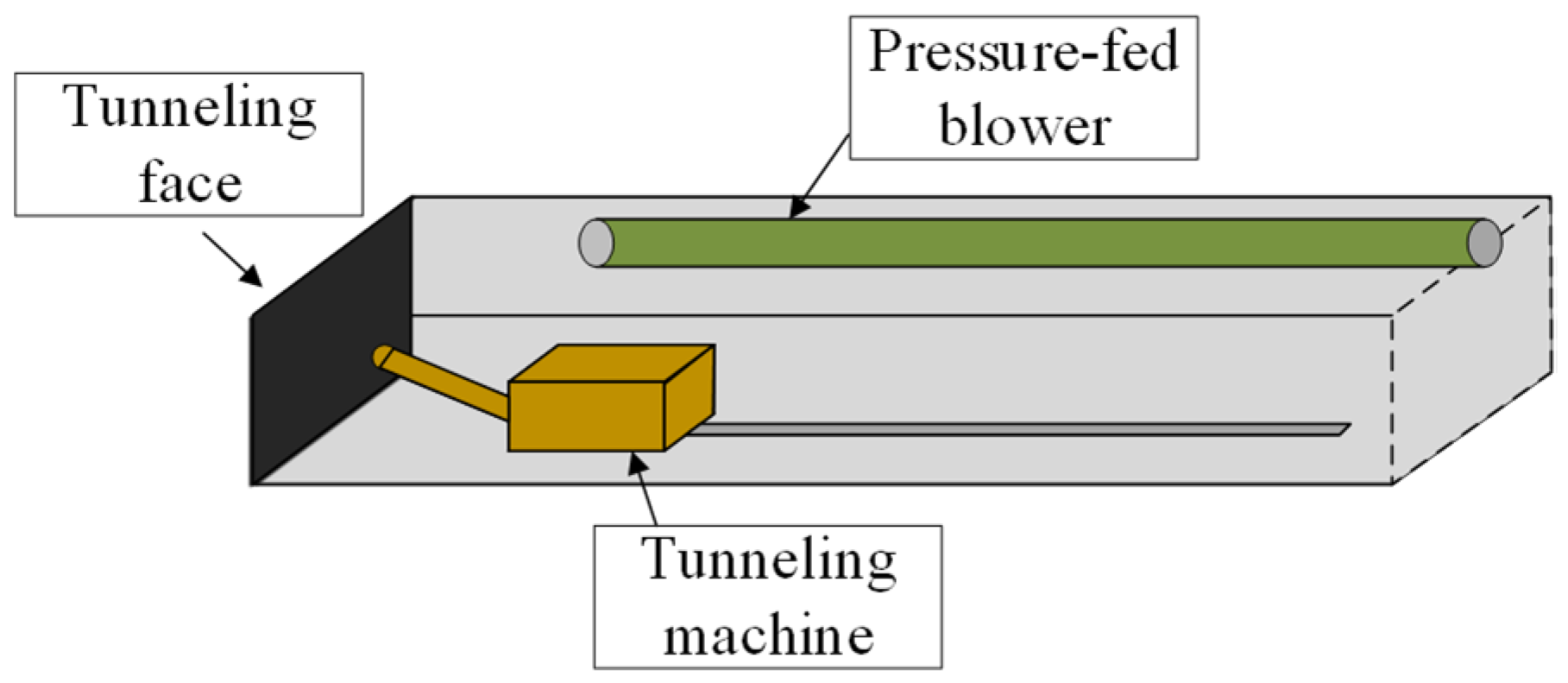
This study was conducted at a coal and gas outburst mine in Changzhi, Shanxi, characterized by complex geology and substantial gas reserves, marking it as high-risk. The test site is in the No. 3 coal mining area. The roadway model is depicted in Figure 1. The tunneling face measures 278 m in strike length and 2175 m in dip length, with a burial depth of 501 to 590 m and a coal seam thickness of 2.1 to 3.7 m. Forced ventilation is utilized. The absolute gas emission rate is 27 m³/min, with a relative emission rate of 5 m³/t. The original gas content ranges from 11 to 14 m³/t, and the coal seam gas pressure is between 1 and 1.3 MPa, indicating high-gas dynamic characteristics. Data collection spanned from 1 March to 1 April 2025, capturing multi-source information. Gas data were recorded every second, totaling 43,000 samples. The physical correlation between the mining equipment parameters and gas dynamics is mainly reflected in the cutting and ventilation processes of the tunneling machine. The cutting current of the roadheader indicates the real-time load and penetration resistance during coal or rock breaking. When the cutting current increases, it implies stronger mechanical disturbance to the coal seam, which enhances gas desorption and migration from the fracture surfaces, thereby leading to a temporary rise in the local gas concentration. Similarly, a higher cutting speed and temperature can accelerate coal fragmentation and increase the exposed surface area, further facilitating gas release. Conversely, a stable current and moderate cutting conditions correspond to steady gas emission rates. Therefore, the equipment parameters can serve as sensitive indicators for transient gas emission behavior and are essential inputs for accurate dynamic gas concentration prediction.

Figure 1. Model diagram of the tunneling face.

The tunneling face data sources are categorized into three main groups: production monitoring data, encompassing parameters like gas concentration, carbon monoxide levels, temperature, and wind speed; equipment monitoring data, including the roadheader’s cutting current, cutting temperature, and mining speed; and gas geological data, such as the coal seam’s gas extraction content. The comprehensive on-site data collected in this study effectively characterizes the dynamic interplay between gas occurrence, ventilation conditions, equipment performance, and operational conditions.

2.2. Feature Extraction

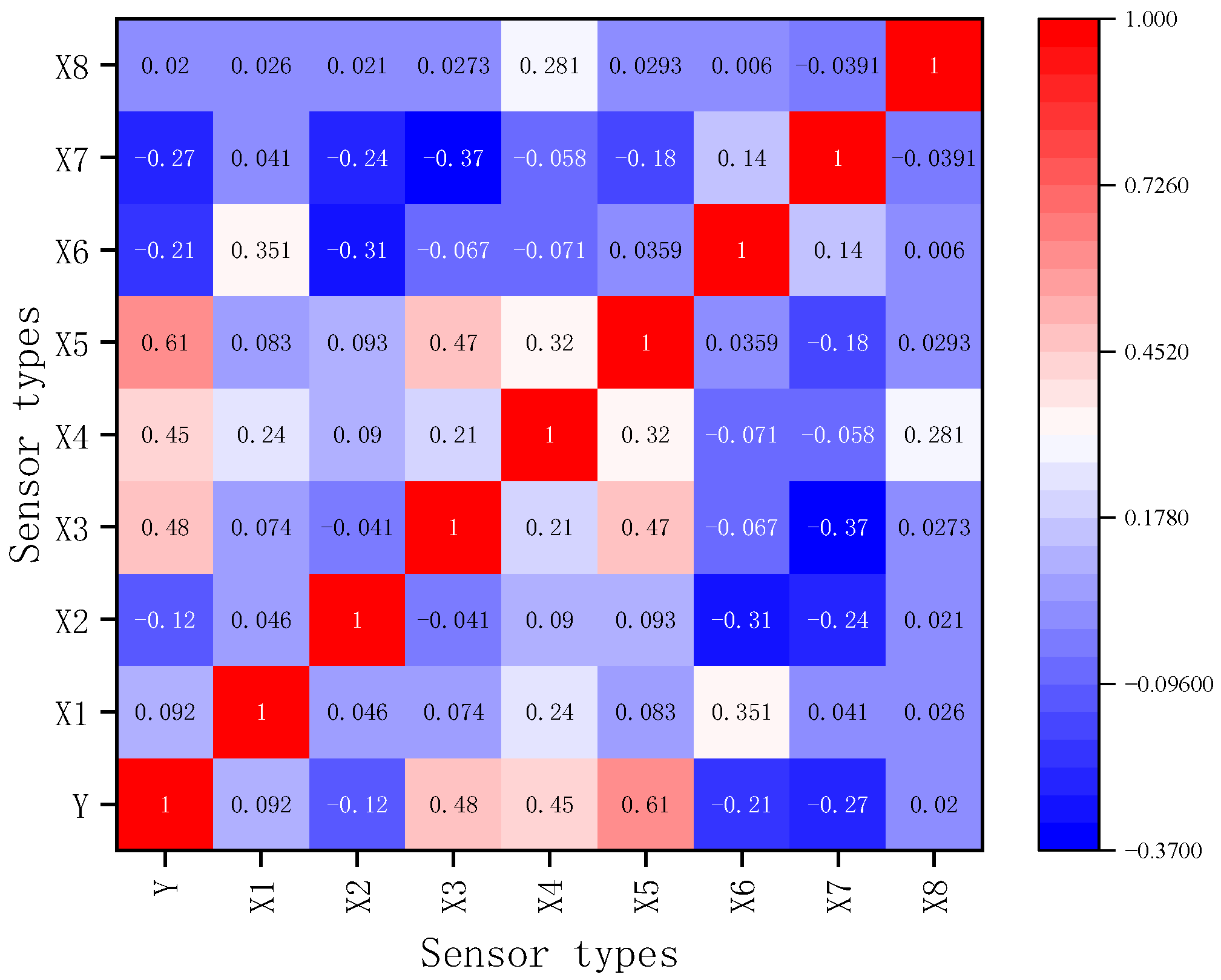
To reveal the interrelationships among various monitoring features, this paper conducts a correlation analysis on the gas concentration and relevant characteristic parameters at the tunneling face. The Spearman correlation coefficient is an index for measuring the similarity between variables. Compared with the Pearson correlation coefficient, this method neither requires the variables to follow a normal distribution nor assumes a linear relationship between variables. Therefore, it can more effectively measure the correlation when the relationship pattern between variables is unclear. Here, $R(x_i)$ and $R(y_i)$ are the rank statistics of variables $X$ and $Y$, $\overline{R(X)}$ and $\overline{R(Y)}$ are the statistical means of variables $X$ and $Y$, and $\rho$ is the Spearman correlation coefficient between the two variables. The judgment criteria for evaluating the correlation between variables using the Spearman correlation coefficient are the same as those of the Pearson correlation coefficient: the closer the absolute value of the coefficient is to 1, the stronger the correlation between variables; the closer it is to 0, the weaker the correlation; if the coefficient is 0, it is considered that there is no correlation between variables.

$$\rho ={\displaystyle \frac{{\displaystyle \sum _{i=1}^n}(R(x_i)-\overline{R(X)})(R(y_i)-\overline{R(Y)})}{\sqrt{{\displaystyle \sum _{i=1}^n(}R(x_i)-\overline{R(X)}{)}^2}\cdot \sqrt{{\displaystyle \sum _{i=1}^n(}R(y_i)-\overline{R(Y)}{)}^2}}}$$

(1)

Figure 2 presents a heatmap of the Spearman correlation coefficients. The x- and y-axes of Figure 2 represent the nine monitoring variables, numbered 1–9, corresponding to tunneling face gas concentration (Y), tunneling footage (X1), fan intake air gas (X2), return air gas (X3), roadheader cutting current (X4), gas on the leeward side of the return airway drill (X5), wind speed (X6), temperature (X7), and carbon monoxide (X8). This clarification has been added to the figure caption in the revised manuscript.

Figure 2. Spearman correlation coefficient heatmap.

This paper identifies the return air gas, roadheader cutting current, leeward side gas of the drilling rig in the return airway, wind speed, and temperature as key parameters for predicting the gas concentration at the heading face. The readings from each sensor are shown in the data sample in Table 1.

Table 1. Data sample.

Time Stamp	Y (%)	X1 (m)	X2 (%)	X3 (%)	X4 (A)	X5 (%)	X6 (m/s)	X7 (°C)	X8 (ppm)
2025-03-19 03:07	0.49	32.5	0.11	0.28	52.8	0.32	3.81	27.40	4.00
2025-03-19 03:08	0.49	32.5	0.11	0.28	50.9	0.32	3.78	27.40	4.00
2025-03-19 03:09	0.51	32.5	0.11	0.26	50.2	0.33	3.80	27.40	4.00
2025-03-19 03:10	0.51	32.5	0.11	0.27	50.5	0.33	3.85	27.40	4.00
2025-03-19 03:11	0.51	32.5	0.11	0.28	50.2	0.33	3.86	27.40	4.00
2025-03-19 03:12	0.52	32.5	0.13	0.28	50.1	0.34	3.82	27.40	4.00
2025-03-19 03:13	0.52	32.5	0.13	0.28	49.9	0.34	3.89	27.40	4.00
2025-03-19 03:14	0.52	32.5	0.13	0.28	50	0.34	3.90	27.40	4.00
2025-03-19 03:15	0.54	32.5	0.11	0.31	50.2	0.32	3.91	27.40	4.00
2025-03-19 03:16	0.54	32.5	0.11	0.31	50.1	0.32	3.86	27.40	4.00

2.3. Data Preprocessing

The subterranean conditions of coal mines are intricate and variable. Sensor data are frequently compromised by physical factors like electromagnetic interference, dust, humidity, and vibration, as well as by unstable transmission, resulting in missing values and outliers. Additionally, challenges arise from inconsistent sampling frequencies and significant dimensional disparities among multi-source heterogeneous data. To ensure accurate model training and reliable predictions, preprocessing of feature data is essential. This study employs direct deletion for isolated missing values and exponential smoothing for continuous ones. Upon detecting a missing value, error calculation is bypassed, yet the model’s smoothing equation is used to recursively compute the level and trend components at the subsequent time point, thus generating an estimate to fill the gap. Outliers are identified using box plots. First, the first quartile (25th percentile) Q1 and the third quartile (75th percentile) Q2 are obtained. The interquartile range (IQR) is then determined by calculating the difference between the quartiles of the data sample. Subsequently, upper and lower limits are set based on this range to identify outliers, where the upper limit LB is calculated as $\mathrm{LB}={\mathrm{Q}}_1-1.5\times \mathrm{IQR}$, and the lower limit UB is calculated as $\mathrm{UB}={\mathrm{Q}}_3+1.5\times \mathrm{IQR}$.

The Kalman filter algorithm is employed to enhance the accuracy of sensor data acquisition by mitigating random noise and measurement errors. This algorithm, rooted in the state–space model, attains optimal estimation through iterative prediction and updating processes. In this study, the process noise covariance (Q) and observation noise covariance (R) for the Kalman filter were set to 0.01 and 0.1, respectively. These parameters were selected through empirical tuning on the training data via a grid search over plausible ranges (Q: 0.001~0.1, R: 0.01~1). The chosen values strike a balance between effectively smoothing high-frequency noise and preserving the true dynamic trends of the gas concentration. When both the state transition matrix and observation matrix are set to 1, Equations (2) and (3) present the predicted state alongside the prediction error covariance, where ${\widehat{x}}_k$ is the state estimate at the current time, and $P_k^{-}$ is the prediction error covariance at the current time.

$${\widehat{x}}_k={\widehat{x}}_{k-1}$$

(2)

$$P_k^{-}=P_{k-1}+Q$$

(3)

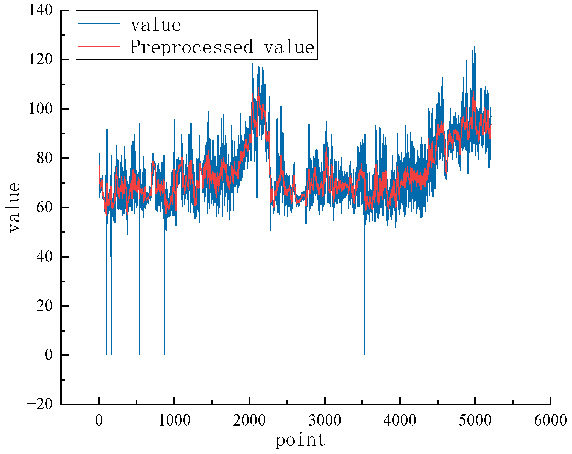
During the update process, the state estimates are corrected by the observed data $z_k$ and ${\widehat{x}}_k^{-}$ predicted state estimates, and new error covariances are recalculated. $K_k$ denotes the Kalman gain, which is used to measure the weight relationship between the predicted values and observed values and gives a modified state estimate based on the predicted states and observed values ${\widehat{x}}_k$. Equation (6) denotes the revised error covariance, while the ultimate data preprocessing steps are illustrated in Figure 3. The figure visually demonstrates the effective suppression of high-frequency noise and abnormal data values resulting from the preprocessing procedure described above, with all major dynamic trends and essential features of the initial signal being faithfully preserved. To quantitatively evaluate the effectiveness of the data quality enhancement, we calculated the signal-to-noise ratio (SNR) before and after filtering. The results indicate an SNR of 27.59 dB, confirming the efficacy of the noise reduction process.

$$K_k={\displaystyle \frac{P_k^{-}}{P_k^{-}+R}}$$

(4)

$${\widehat{x}}_k={\widehat{x}}_k^{-}+K_k(z_k-{\widehat{x}}_k^{-})$$

(5)

$$P_k=(1-K_k)P_k^{-}$$

(6)

Figure 3. Data preprocessing effect diagram.

3. Gas Concentration Prediction Model Based on KAN-iTransformer

3.1. Overall Model Process

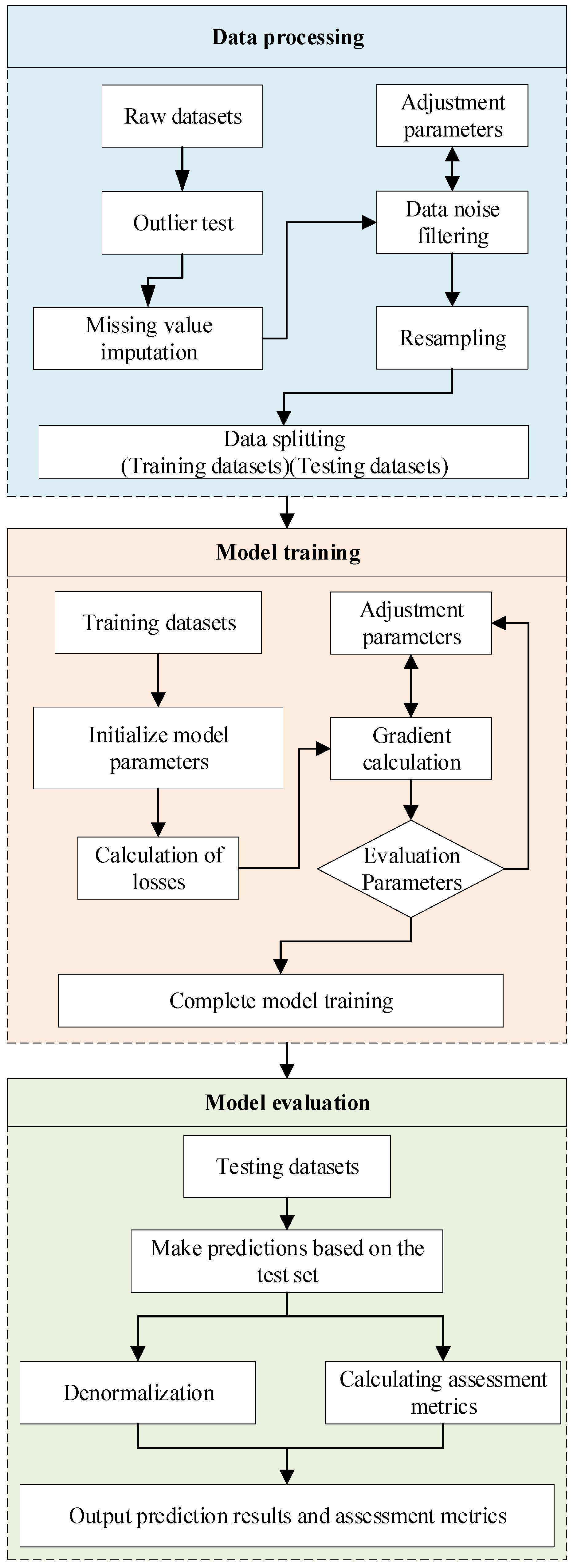
The framework for constructing the gas concentration prediction model is depicted in Figure 4, comprising three main stages: data processing, model training, and model evaluation. Initially, the dataset undergoes preprocessing, as described in Section 2.3, to ensure modeling reliability. Subsequently, feature variables are resampled based on the sampling frequency, aligning all feature data with the tunneling face gas concentration data. The data are then split into training and test sets in an 8:2 ratio.

Figure 4. Overall model flowchart.

The model training phase involves five key steps. Initially, the training dataset is loaded, and model parameters are set. Next, the loss is computed by comparing the model’s predictions with the true input values. The model performance is enhanced through gradient calculations and loss function optimization, with continuous adjustment of the hyperparameters based on the evaluation metrics to achieve optimal training outcomes. In the evaluation phase, predictions are made using the test set, followed by inverse normalization to yield the actual predicted gas concentration values. Finally, performance metrics like MSE, MAE, and MAPE are computed to thoroughly assess the model’s accuracy and generalization capability.

3.2. KAN Model Architecture

The Kolmogorov–Arnold Network (KAN) is an innovative neural network architecture introduced in accordance with the Kolmogorov–Arnold representation theorem [16]. This theorem asserts that any multivariate function can be expressed as a composite of finite continuous univariate functions and additive operations. In KAN, traditional linear weights are substituted with adaptable one-dimensional functions, typically defined by B-splines. The network’s nodes exclusively execute summation operations, while nonlinearity is exclusively achieved through the functions situated on the network’s edges.

Traditional multilayer perceptrons (MLPs) place simple, fixed weights along the network’s edges while performing complex nonlinear computations (such as the ReLU function) within the neural nodes. This can be visualized as a network composed of fixed pipes (edges) and intelligent valves (nodes). In contrast, the Kolmogorov–Arnold Network (KAN) performs a ‘functional inversion’: it places simple summation operations on the nodes while assigning complex learnable nonlinear functions to each edge of the network. This effectively transforms the network into a system composed of flexible malleable smart pipes (edges) and simple convergence points (nodes). The advantage of this structure lies in KAN’s ability to learn and represent complex nonlinear relationships with fewer parameters and higher accuracy. In gas prediction tasks, this means the model can capture the subtle dynamically changing physical relationship between covariates and gas concentration more flexibly and precisely than approximating it with fixed piecewise linear functions.

When provided with input vector $x^{\left(l\right)}\in R^{n_l}$ at layer $l$ and output $x^{\left(l+1\right)}\in R^{n_{l+1}}$, along with a univariate function ${\varphi }_{j,i}^{(l)}$ associated with each connected edge, the input at layer $l+1$ can be represented by Equation (7). The computation formula for $\varphi \left(x\right)$, as depicted in Equation (8), comprises a linear combination of residual basis functions and B-splines, where $c_k$ represents a trainable coefficient, and $B_k\left(x\right)$ denotes the B-spline basis function.

$$x_j^{(l+1)}={\displaystyle \sum _{i=1}^{n_l}{\varphi }_{j,i}^{(l)}}(x_i^{(l)}),\hspace{1em}j=1,\dots ,n_{l+1}$$

(7)

$$\varphi \left(x\right)=w_b\cdot silu\left(x\right)+w_s{\displaystyle \sum _k{c}_k}{B}_k\left(x\right)$$

(8)

3.3. Improve the Architecture of the iTransformer Model

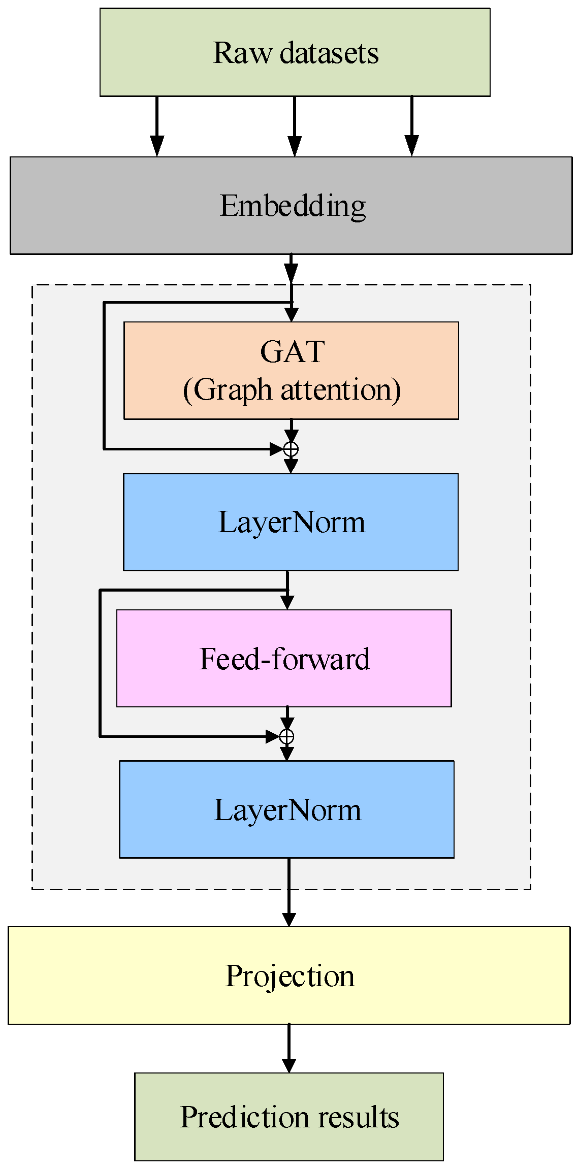
The gas concentration prediction model in this study employs the inverted Transformer (iTransformer), which introduces a novel tokenization scheme for multivariate time series [17]. Unlike traditional methods that treat each time step as an independent token [18], iTransformer considers the entire historical sequence of each variable as a single token. This approach redirects the self-attention mechanism’s focus from the temporal to the variable dimension, facilitating explicit modeling of inter-variable relationships. As depicted in Figure 5, the architecture comprises three key components: an embedding layer, an inverted Transformer module, and a prediction head.

Figure 5. Model structure diagram.

The standard Transformer treats each time point as an independent token when processing multi-variable time series. It then uses attention mechanisms to identify relationships between different time points. In contrast, our iTransformer adopts an ‘inverted’ perspective. It treats the entire historical sequence of each variable—for example, all readings of ‘return air methane’ from inception to the present—as a single complete (token). Its attention mechanism then analyzes the intrinsic connections between covariate tokens and target variable tokens. This approach directly shifts the computational focus from the temporal dimension to the variable dimension, enabling us to explicitly model and understand the dynamic dependencies between different sensor signals. This is crucial for comprehending the multi-factor driving mechanisms of gas migration.

3.3.1. Embedded Layer

In the context of multivariate time series prediction, historical monitoring data are denoted as follows: $X=\{x_1,\dots ,x_T\}\in {ℝ}^{T\times N}$ denotes the representation of the data, where $T$ signifies the time span, and $N$ indicates the number of variables. Unlike conventional Transformers that assign tags along the time axis, the Transformer model incorporates all variables simultaneously as tags. Specifically, iTransformer redefines tags along the variable axis. Each variable’s entire historical sequence, denoted as $X_{:,n}\in {ℝ}^T$, is treated as a singular variable marker. The embedding procedure is mathematically defined in Equation (9), and the resultant embedding vectors are concatenated according to Equation (10). By encoding the complete time series of each variable as an individual variable label, iTransformer circumvents issues such as time misalignment and correlation loss that arise from amalgamating all variables under time labels in traditional methodologies.

$$h_n^{(0)}=\stackrel{\cdot }{f_{\mathrm{emb}}}(X_{:,n}),\hspace{1em}n=1,\dots ,N$$

(9)

$$H^{(0)}=[h_1^{(0)},h_2^{(0)},\dots ,h_N^{(0)}]\in {ℝ}^{N\times D}$$

(10)

3.3.2. Improved Inverted Transformer Module

The inversion Transformer module comprises layer normalization, a feedforward network, and graph attention components. To address the non-stationarity and scale heterogeneity of gas monitoring variables, time horizon normalization (TLN) is integrated within each inverted Transformer module. In contrast to the base Transformer’s normalization across feature dimensions at every time step, TLN normalizes along the time dimension of each variable sequence. This approach effectively mitigates the issue of time misalignment among multiple variables.

Specifically, the representation for variable $n$ is calculated as Equation (11), where ${\mu }_n$ and ${\sigma }_n^2$ are the mean and standard deviation calculated along the timeline of variable $n$.

$${\tilde{h}}_{n,t}={\displaystyle \frac{h_{n,t}-{\mu }_n}{{\sigma }_n}}$$

(11)

$${\mu }_n={\displaystyle \frac{1}{T}}{\displaystyle \sum _{t=1}^T{h}_{n,t}}$$

(12)

$${\sigma }_n^2={\displaystyle \frac{1}{T}}{\displaystyle \sum _{t=1}^T{\left(h_{n,t}-{\mu }_n\right)}^2}$$

(13)

Following the attention mechanism and layer normalization, each variable token is processed through a feed-forward network (FFN) to enhance its temporal representation. Unlike the FFN in the standard Transformer model, which processes tokens at each time point, this FFN specifically models temporal dependencies within a single variable, as each token encompasses the entire historical window of that variable. This approach extracts complex nonlinear relationships within the variable, enabling the collaborative learning of common temporal patterns like seasonality, periodicity, and transient shocks.

In the original iTransformer model, self-attention is utilized along the variable dimension, with each variable token representing the historical sequence measured by sensors. While this design effectively captures inter-variable dependencies, it does not account for the non-random distribution of monitoring sensors in underground coal mines. These sensors are strategically placed along excavation roadways, ventilation paths, and near mining equipment. Consequently, gas concentration dynamics are heavily influenced by the airflow topology, roadway connectivity, and the spatial proximity of sensors.

Substituting the original self-attention mechanism with a graph attention mechanism within the inverted Transformer module [19] exploits the spatial topology of each sensor and incorporates spatial prior knowledge. Attention aggregation is confined to adjacent nodes with physical or statistical relevance, thus preventing the formation of false dependencies between distant or unrelated variables. This approach markedly improves the model’s inductive capability, making it especially effective for tackling the challenges of multi-sensor gas concentration prediction.

Each variable labeled $h_i\in {ℝ}^D$ is treated as a node in the graph $G=(V,E)$, where edge set $E$ encodes one of three relationships: (1) physical network topology, (2) spatial proximity of sensors, or (3) associations between variables with statistically significant correlations.

This paper employs mine ventilation system diagrams and statistically significant correlations between variables as criteria for selecting edge sets. If two sensors are located on the same ventilation flow path with a clear airflow connection, they are considered physically connected. This key prior knowledge of roadway connectivity is incorporated into the model as a hard constraint.

Based on the pairwise correlation strengths between the variables identified in Section 2.2, only variable pairs with the largest absolute correlation coefficients are retained. This approach effectively identifies pairs exhibiting strong synergistic variation patterns, such as “roadheader current” and “tunneling face methane”. The final graph structure used for the graph attention network is the union of these two adjacency relationships. Any connection confirmed by either criterion is retained in the graph. This integrated construction strategy ensures the model strictly adheres to the physical constraints of mine ventilation while adaptively learning significant statistical correlations revealed in the data. This guarantees both the physical consistency and dynamic adaptability of the constructed graph structure.

For each connected node $(i,j)\in E$, we update the node characteristics as shown in Equation (14), where $W$ is the learnable weight matrix, $\sigma \left(\cdot \right)$ is the activation function, and $E(i)$ represents the set of adjacent nodes of node $i$. It is particularly noteworthy that, in the graph attention network employed in this study, the final connection strength between nodes is not a static predefined value but is dynamically computed through the attention mechanism. For any central node, the connection strength with all neighboring nodes is calculated as shown in Equation (15), where ${\alpha }_{ij}^{(l)}$ represents the final contribution or connection strength of node $j$’s features to node $i$, and its calculation formula is shown in (15), where $a$ is the learnable attention vector, and $\parallel$ represents the vector splicing operation.

$$h_i^{(l+1)}=\sigma \left({\displaystyle \sum _{j\in E(i)}{\alpha }_{ij}^{(l)}}W{h}_j^{(l)}\right)$$

(14)

$${\alpha }_{ij}^{(l)}={\displaystyle \frac{\exp \left(\mathrm{LeakyReLU}(a^{\top }[W{h}_i^{(l)}\parallel W{h}_j^{(l)}])\right)}{{\displaystyle \sum _{k\in E(i)}\exp }\left(\mathrm{LeakyReLU}(a^{\top }[W{h}_i^{(l)}\parallel W{h}_k^{(l)}])\right)}}$$

(15)

To augment the model’s expressive capacity, we introduce a multi-attention mechanism, as illustrated in Equation (16), where $M$ represents the number of attention heads, and $W^{(m)}$ and ${\alpha }^{(m)}$ are unique parameters associated with each head.

$$h_i^{(l+1)}={\Vert }_{m=1}^M\sigma \left({\displaystyle \sum _{j\in \mathcal{N}(i)}{\alpha }_{ij}^{(l,m)}}{W}^{(m)}{h}_j^{(l)}\right)$$

(16)

Following the graph attention update, the output is processed by the feed-forward network. This enhanced approach integrates graph-based constraints within the iTransformer architecture, aligning cross-variable dependencies with the spatial topology and physical principles of sensors. By incorporating the topological data of coal mine sensors, the model effectively captures both local variable correlations and global dependencies, thereby improving the physical consistency and robustness of underground gas concentration predictions.

3.3.3. Prediction Header

In the initial Transformer model, the ultimate label $h_n^{(l)}$$\in {ℝ}^D$ is extended to the subsequent forecasting interval via a regression network, as opposed to the original approach employing a multilayer perceptron for this purpose. To enhance the model’s capacity to dynamically characterize profoundly nonlinear and non-stationary data, such as gas concentration in coal mines, we substitute the multilayer perceptron with KAN and incorporate spline basis function expansion to augment the model’s capability for nonlinear expression. As delineated in Section 2.2, the ultimate predictive value is denoted by Equation (17), where $S$ signifies the time step under prediction.

To address potential instability in KAN training, we employed L1 regularization on spline coefficients to promote function smoothness and normalized the input data. Concurrently, dynamic learning rate scheduling based on validation set loss was adopted during training.

The hyperparameters of the KAN model were determined through a combination of theoretical considerations and empirical validation. Structural parameters (depth, width) were selected via grid search to balance model capacity and training stability. Spline parameters (grid size, order, smoothness λ) were tuned to ensure sufficient nonlinear expressiveness without overfitting. Training parameters (learning rate, weight decay, dropout) were optimized according to the validation loss. The final configuration (depth = 3, width = 128, grid size = 10, spline order = 3, λ = 1 × 10⁻³, learning rate = 1 × 10⁻³) consistently yielded stable convergence and the best predictive performance across datasets. The early stopping method was employed to introduce dropout layers within KAN’s internal components to address model overfitting. Weight decay was configured within the optimizer, establishing a multi-level regularization strategy that collectively ensures the model’s generalization capability.

$${\widehat{y}}_s={\displaystyle \sum _{i=1}^D{\varphi }_i^{(s)}}(h_{n,i}^{(L)}),\hspace{1em}s=1,2,\dots ,S$$

(17)

4. Experimental Results and Analysis

4.1. Model Evaluation and Experimental Configuration

The gas concentration prediction model, utilizing the improved KAN-iTransformer, was trained on a system featuring an Intel Core i7-11850H processor (3.25 GHz), 32 GB RAM, and an NVIDIA T600 GPU. The model employed the mean squared error (MSE) loss function, comparing predicted and actual gas concentration values. Training utilized the Adam optimizer with a learning rate of 0.001, a weight decay of 0.00001, and an early stopping mechanism.

We allocated the initial 80% of the dataset for training and the remaining 20% for testing. Post feature construction, the data were fed into the gas concentration prediction model to perform multi-step forecasts of future gas concentrations in the test area at one-minute intervals. The model performance was assessed using MSE, MAE, and MAPE metrics.

$$\mathrm{MSE}={\displaystyle \frac{1}{N}}{\displaystyle \sum _{i=1}^N{\left(y_i-{\widehat{y}}_i\right)}^2}$$

(18)

$$\mathrm{MAE}={\displaystyle \frac{1}{N}}{\displaystyle \sum _{i=1}^N|y_i-{\widehat{y}}_i|}$$

(19)

$$\mathrm{MAPE}={\displaystyle \frac{100\%}{n}}{\displaystyle \sum _{i=1}^n\left|\frac{y_i-{\widehat{y}}_i}{y_i}\right|}$$

(20)

4.2. Comparative Analysis of Single-Step Forecasting Performance Across Models

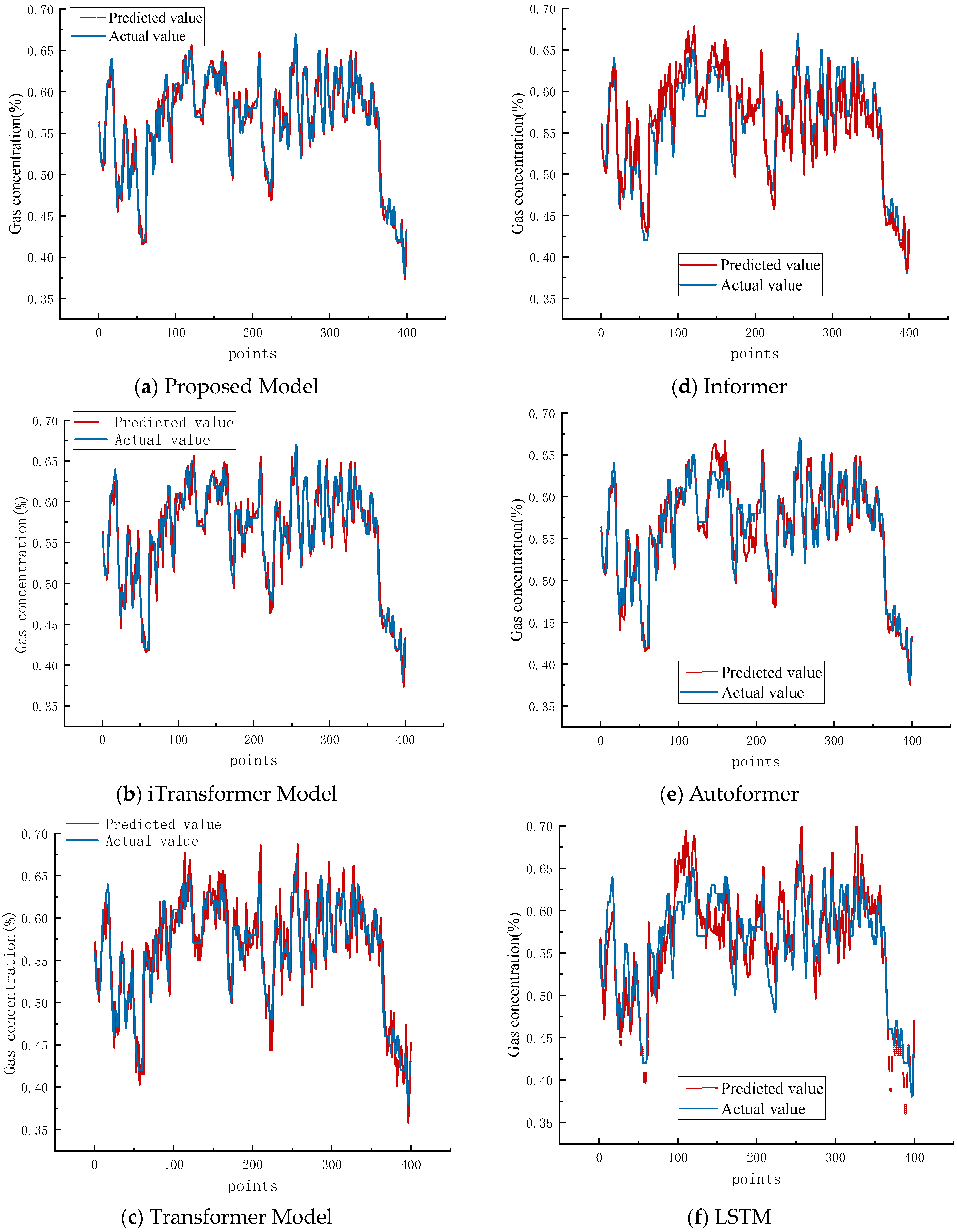
Figure 6 compares the model’s predictions with actual values for gas concentration at the tunneling face. The proposed model demonstrates exceptional accuracy over 400 time steps, each representing a one-minute interval. The red prediction curve closely aligns with the blue curve of real data, capturing the fluctuations in gas concentration across various time points. During periods of rapid change, the model accurately predicts both the trends and the amplitude of peaks and valleys. In phases of gradual change, the model’s predictions exhibit minor periodic fluctuations with minimal deviation. Notably, when the actual data show a sharp decline from 0.58 to approximately 0.40, the prediction curve mirrors this downward trend synchronously.

Figure 6. Comparison of single-step prediction results across models.

The comparison reveals that while the iTransformer model captures the general trend of gas concentration fluctuations, it produces numerous instantaneous spikes and inaccurately predicts the change amplitude. Conversely, the Transformer model exhibits noticeable deviations and lags in its predictions. As actual concentrations begin to rise or fall, the model’s predictions remain at previous levels. Even when real data show minimal fluctuations, the predicted values still exhibit local variations and deviate from reality, indicating the model’s inability to effectively capture dynamic temporal dependencies. From the perspective of real-time prediction, such delayed or oscillatory responses can lead to false or missed warnings in underground monitoring systems. In contrast, the proposed KAN-iTransformer demonstrates faster adaptive response to transient concentration changes and smoother temporal evolution, which are essential for ensuring stable and timely prediction in real coal-mine operations.

Table 2 presents a comprehensive comparison of performance indicators for single-step prediction among different models, including the newly added state-of-the-art time series models (iTransformer, Transformer, Informer, Autoformer, LSTM). The proposed model demonstrates superior performance across all metrics when compared to all baseline models. Specifically, the mean squared error (MSE) of the proposed model is 0.000307, representing significant reductions of 14.2%, 45.3%, 25.2%, and 37.1% compared to the iTransformer, Transformer, Informer, and Autoformer models, respectively. The performance advantage over the classical LSTM model is even more pronounced, with a 66.5% reduction in MSE.

Table 2. Comparative analysis of single-step prediction performance.

Model	MSE	MAE	MAPE	R2
Improved iTransformer	0.000307	0.012921	2.321373	0.916450
iTransformer	0.000358	0.014020	2.511322	0.882508
Transformer	0.000562	0.018397	3.320037	0.846822
Informer	0.000412	0.026127	4.6949	0.806608
Autoformer	0.000488	0.024723	4.4184	0.823428
LSTM	0.000917	0.037535	6.7352	0.708254

Similarly, the mean absolute error (MAE) of the proposed model is 0.012921, indicating decreases of 7.8%, 29.8%, 50.5%, and 47.7% relative to the iTransformer, Transformer, Informer, and Autoformer models, respectively. The mean absolute percentage error (MAPE) of the proposed model is approximately 2.32%, indicating that, on average, the predictions deviate by only 2.32% from the true values. This value is notably lower by 7.6%, 30.1%, 50.6%, and 47.5% compared to the iTransformer, Transformer, Informer, and Autoformer models, respectively.

Furthermore, the coefficient of determination (R²) for the proposed model is notably high at 0.9164, surpassing the values of all comparison models. The substantial improvement over recent temporal models like Informer and Autoformer demonstrates the effectiveness of our proposed architectural enhancements in capturing the complex spatiotemporal dependencies in gas concentration data.

4.3. Model Multi-Step Prediction Performance Comparison Analysis

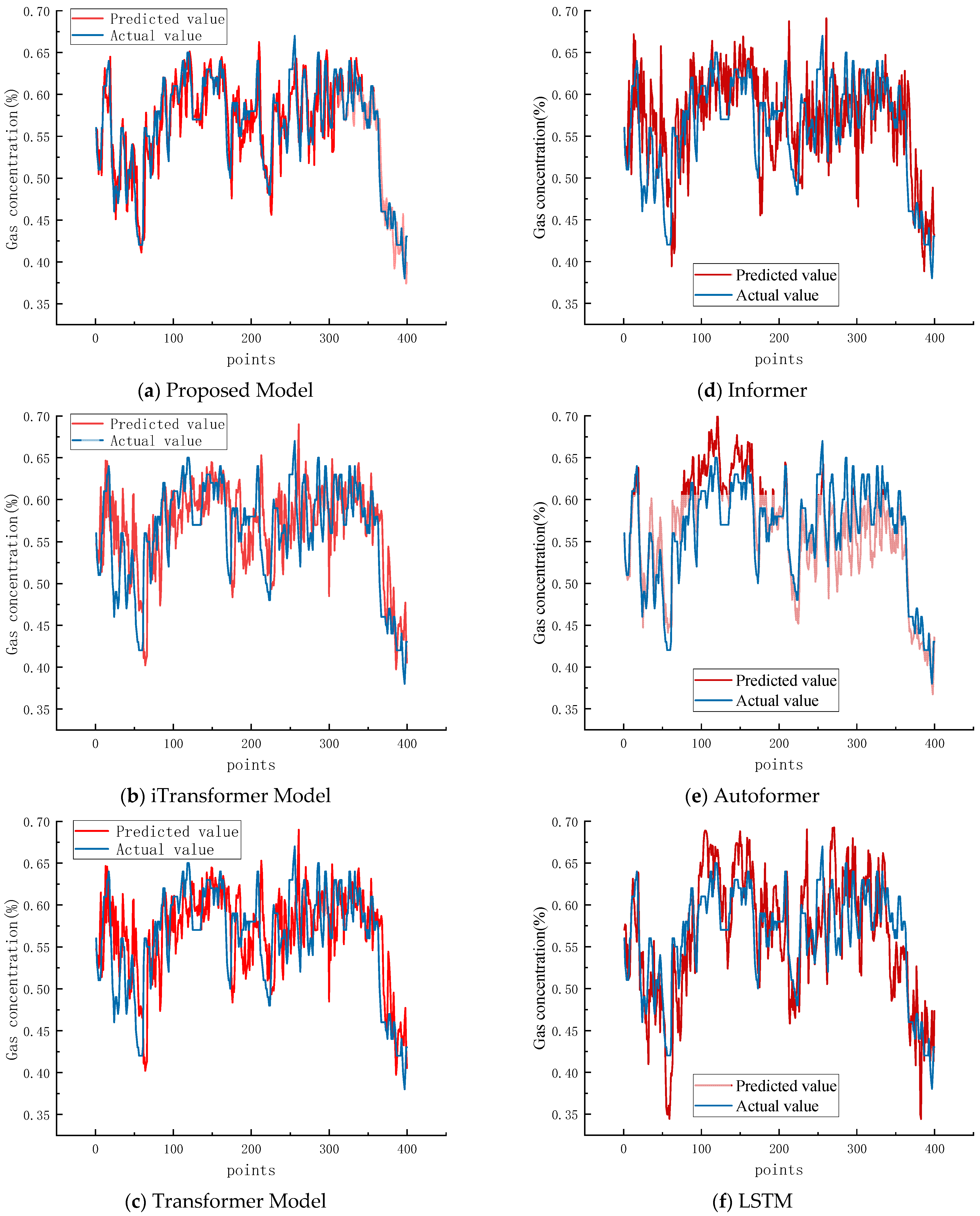
To validate the model’s performance in multi-step gas concentration prediction, we analyzed its effectiveness with a step size of 10. Figure 7 illustrates the comparison results. The model exhibits fluctuations of varying magnitudes and minor local errors compared to single-step predictions. Nonetheless, it maintains a strong ability to fit the data trend, accurately predicting the overall trajectory of gas concentration changes. In contrast, the prediction curves of the other models display significant systematic deviations and attenuated fluctuations relative to the actual values. While the predicted values of Informer and Autoformer approximate the real situation during steady changes, they diverge notably during sharp increases or decreases, showing a pronounced lag effect. The Transformer and LSTM models exhibit the poorest performance, with substantial deviations throughout the prediction horizon.

Figure 7. Comparison of multi-step prediction results across models.

Table 3 presents a comprehensive comparison of the performance indicators for multi-step predictions across all models, unequivocally demonstrating the superior performance of our proposed model. The model’s MSE is 0.000913, which represents remarkable reductions of 63.7%, 80.9%, 69.3%, 66.5%, and 78.1% compared to the iTransformer, Transformer, Informer, Autoformer, and LSTM models, respectively. These substantial improvements highlight our model’s exceptional accuracy in long-term forecasting scenarios.

Table 3. Comparative analysis of multi-step prediction performance.

Model	MSE	MAE	MAPE	R2
Improved iTransformer	0.000913	0.022867	4.117202	0.851230
iTransformer	0.002517	0.039033	7.183084	0.706521
Transformer	0.004784	0.052639	9.741005	0.303680
Informer	0.002978	0.046203	7.832372	0.664133
Autoformer	0.002728	0.041250	7.532246	0.689241
LSTM	0.004171	0.071535	11.35268	0.278823

Similarly, the MAE of the proposed model is 0.022867, indicating decreases of 41.4%, 56.5%, 50.5%, 44.6%, and 68.0% relative to the iTransformer, Transformer, Informer, Autoformer, and LSTM models. The MAPE value of 4.117% further confirms the model’s precision, being significantly lower than all comparison models. Notably, the proposed model achieves an R² value of 0.8512, which is only 0.0652 less than the single-step prediction, indicating minimal degradation in fitting ability and ensuring both short-term accuracy and long-term stability.

4.4. Model Emergency Response Mechanism

In the intricate setting of a coal mine heading face, errors and uncertainties are inherent in the multi-step prediction of gas concentration. Relying solely on singular point predictions and fixed threshold values for exceeding limits can lead to erroneous alerts. This study introduces prediction intervals following multi-step predictions to assess the uncertainty in model predictions by analyzing the distribution characteristics of the prediction residuals. For instance, at a 95% confidence level, the kth step prediction interval is expressed as shown in Equation (21), where ${\widehat{y}}_{t+k}^{\left(L\right)}$ and ${\widehat{y}}_{t+k}^{\left(U\right)}$ represent the upper and lower confidence intervals, respectively, with a confidence level of 95%.

$${\widehat{y}}_{t+k}^{\left(L\right)}\le y_{t+k}\le {\widehat{y}}_{t+k}^{\left(U\right)}$$

(21)

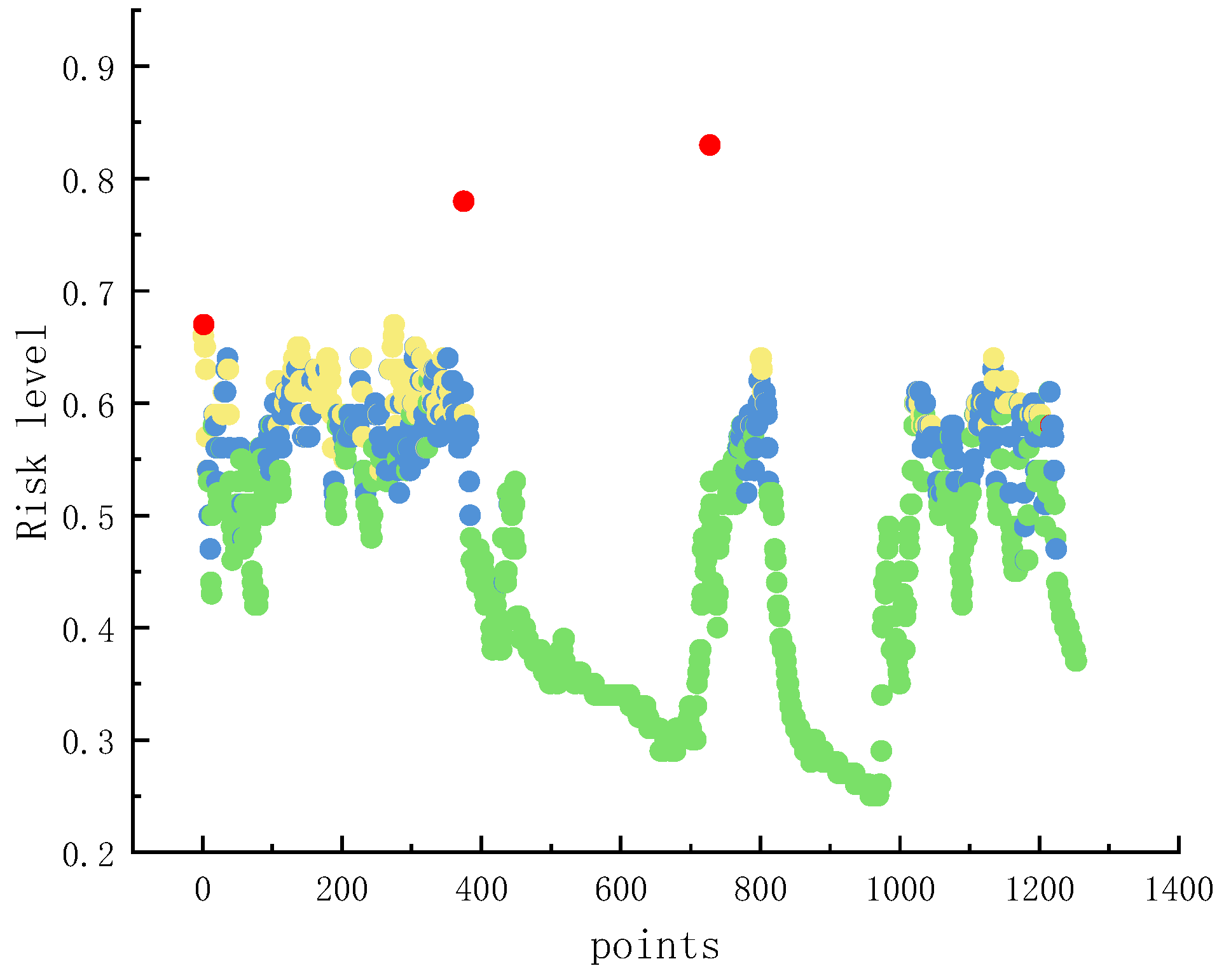
Setting a confidence threshold for gas concentration exceedances yields the emergency response grading shown in Figure 8. When the predicted mean falls below the threshold, and the entire confidence interval remains within the safe range, it is classified as green level, requiring no emergency measures. When the upper confidence limit exceeds the threshold, but point predictions remain within the safe range, it is classified as a blue level, indicating a potential risk phase. Enhanced monitoring of methane concentrations in the area and increased frequency of portable methane detector checks are recommended. When the predicted mean exceeds the threshold, but the lower bound of the interval remains below the threshold, it is classified as an orange level, indicating a general risk phase. Preventive ventilation measures to enhance extraction efficiency are required. The procedures mandate that upon receiving an alert, safety officers must conduct on-site verification using independent data sources such as portable gas detectors and video surveillance. This human–machine collaborative process ensures final decision-making, fundamentally eliminating production losses caused by misjudgments from single models. To prevent false alarms, the system incorporates a simple delayed confirmation logic. For instance, an “orange” risk level is only formally triggered after persisting for at least two prediction cycles (2 min), filtering out transient false alarms caused by signal fluctuations. When the entire prediction interval exceeds the threshold—meaning the lower confidence bound also surpasses the threshold—the risk is classified as red. This indicates a high-risk phase requiring immediate verification of all sensor functionality and preparation for mandatory emergency measures, including equipment shutdown and personnel evacuation.

Figure 8. Visualization of emergency response grading.

The early warning mechanism proposed in this study possesses second-level inference capabilities, meeting the real-time requirements of mine monitoring. Technically, it is recommended to retrieve real-time data from the safety monitoring system via the OPC UA protocol. After completing risk prediction at the edge computing node, tiered warning signals are pushed to the integrated automation platform through RESTful API, triggering a graded response ranging from audible–visual alerts to forced power shutdown. This solution, based on industrial standard protocols, clearly defines hardware deployment and system interface requirements, providing a clear and feasible technical path for industrial implementation.

5. Discussion

5.1. Model Generalization

It should be noted that the dataset used in this study was collected from a single high-gas coal mine in Changzhi, Shanxi. Although the geological and operational conditions of this site are representative of typical tunneling faces in gassy coal seams, the model’s generalization ability under different geological structures, gas pressures, and mining processes has not yet been fully verified. Nevertheless, since the proposed KAN-iTransformer integrates both spatial topological features and dynamic inter-variable dependencies through its graph attention and kernel function mechanisms, it has a strong potential for transferability.

Future work will explicitly focus on assessing and enhancing the model’s generalizability. This will involve collecting comprehensive datasets from multiple mines with varying geological characteristics and operational practices. Transfer learning techniques will also be explored to fine-tune the pre-trained model on new smaller datasets from different mines, thereby improving its performance and accelerating its deployment in novel settings.

5.2. Model Limitations and Adaptability Under Extreme Conditions

Although the proposed KAN-iTransformer model demonstrates high prediction accuracy and stability under normal tunneling operations, several limitations remain. First, the model relies on the continuity and quality of sensor data. In cases of abrupt signal loss or severe sensor interference, its performance may degrade. Second, extreme working conditions such as sudden gas outbursts involve complex nonlinear dynamics and rapid physical changes that exceed the range of patterns learned from historical data. Under these circumstances, short-term prediction errors may increase due to insufficient extreme-event samples in the training set.

Nevertheless, the model’s adaptive architecture—combining kernel-based nonlinear mapping and graph attention—allows it to maintain relative robustness when faced with transient disturbances. In future work, the adaptability to extreme conditions will be further improved by incorporating online learning and anomaly-driven model updating strategies, enabling the system to dynamically adjust parameters and respond more effectively to emergency gas events.

6. Conclusions

In response to the challenges such as strong nonlinearity, strong correlation, and spatio-temporal dynamic characteristics in the prediction of gas concentration at coal mine heading faces, this paper proposes a gas concentration prediction model (KAN–iTransformer) that integrates the KAN network and the improved iTransformer. Through the feature extraction and pre-processing of multi-source sensor data, combined with the long-sequence time series modeling and the graph attention mechanism with spatial topology perception, accurate prediction of the gas concentration at the heading face is achieved. The main conclusions are as follows:

(1)

This paper innovatively proposes a gas concentration prediction model for the tunneling face based on the Kernel Attention Network (KAN) and the improved iTransformer. The KAN network replaces the traditional linear weights with a learnable kernel function, enhancing the model’s ability to represent nonlinear relationships. The improved iTransformer effectively captures the long-term dependencies among multiple variables through inverted token construction and graph attention mechanism.

(2)

The experimental results show that in single-step prediction, the mean squared error (MSE) of the proposed model is 0.000307, the mean absolute error (MAE) is 0.012921, the mean absolute percentage error (MAPE) is 2.321373, and the coefficient of determination (R²) reaches 0.916450. Compared with the iTransformer and Transformer models, the error indicators are significantly reduced (the MSE decreases by 14.2% and 45.3%, respectively). More importantly, when compared with other state-of-the-art time series models, our model demonstrates even more substantial improvements, with MSE reductions of 25.2% over Informer, 37.1% over Autoformer, and 66.5% over LSTM. This proves the superiority of the model in capturing transient changes and peak features.

(3)

The proposed model achieves a high prediction accuracy, with an R² value exceeding 0.9, indicating excellent consistency between the predicted and observed gas concentrations. This high level of accuracy ensures that the model can reliably capture the dynamic evolution of harmful gas concentrations in real time. By incorporating prediction interval estimation and graded early-warning mechanisms, the model not only quantifies prediction uncertainty but also enables dynamic multi-level responses to potential gas over-limit events. These capabilities establish a solid foundation for intelligent real-time early warning and decision-making in underground coal mine safety management.

References

- Liu, B.; Chang, H.; Li, Y.; Zhao, Y. Carbon emissions predicting and decoupling analysis based on the PSO-ELM combined prediction model: Evidence from Chongqing Municipality, China. Environ. Sci. Pollut. Res. 2023, 30, 78849–78864. [Google Scholar] [CrossRef] [PubMed]
- Wei, C.; Li, C.; Ye, Q.; Li, Z.; Hao, M.; Wei, S. Modeling of gas emission in coal mine excavation workface: A new insight into the prediction model. Environ. Sci. Pollut. Res. 2023, 30, 100137–100148. [Google Scholar] [CrossRef] [PubMed]
- Bi, S.; Shao, L.; Qi, Z.; Wang, Y.; Lai, W. Prediction of coal mine gas emission based on hybrid machine learning model. Earth Sci. Inform. 2023, 16, 501–513. [Google Scholar] [CrossRef]
- Song, W.; Han, X.; Qi, J. Prediction of gas emission in the tunneling face based on LASSO-WOA-XGBoost. Atmosphere 2023, 14, 1628. [Google Scholar] [CrossRef]
- Ji, P.; Shi, S.; Shi, X. Research on gas emission quantity prediction model based on EDA-IGA. Heliyon 2023, 9, e17624. [Google Scholar] [CrossRef] [PubMed]
- Zeng, J.; Li, Q. Research on prediction accuracy of coal mine gas emission based on grey prediction model. Processes 2021, 9, 1147. [Google Scholar] [CrossRef]
- Yang, Y.; Du, Q.; Wang, C.; Bai, Y. Research on the method of methane emission prediction using improved grey radial basis function neural network model. Energies 2020, 13, 6112. [Google Scholar] [CrossRef]
- Zhang, J.; Cui, Y.; Yan, Z.; Huang, Y.; Zhang, C.; Zhang, J.; Guo, J.; Zhao, F. Time series prediction of gas emission in coal mining face based on optimized Variational mode decomposition and SSA-LSTM. Sensors 2024, 24, 6454. [Google Scholar] [CrossRef] [PubMed]
- Lin, H.; Li, W.; Li, S.; Wang, L.; Ge, J.; Tian, Y.; Zhou, J. Coal mine gas emission prediction based on multifactor time series method. Reliab. Eng. Syst. Saf. 2024, 252, 110443. [Google Scholar] [CrossRef]
- Liang, R.; Chang, X.; Jia, P.; Xu, C. Mine gas concentration forecasting model based on an optimized BiGRU network. ACS Omega 2020, 5, 28579–28586. [Google Scholar] [CrossRef] [PubMed]
- Li, X.; Zheng, W.; Lu, G.; Kang, Y.; Xia, Y.; Zhou, Z. A new time series of gas outburst prediction model and application in coal mine and through-coal-seam tunnel mining face. IEEE Access 2025, 13, 115960–115971. [Google Scholar] [CrossRef]
- Yang, H.; Wang, J.; Zhang, H. Research on Gas Multi-indicator Warning Method of Coal Mine tunneling face Based on MOA-Transformer. ACS Omega 2024, 9, 22136–22144. [Google Scholar] [CrossRef] [PubMed]
- Qu, H.; Shao, X.; Gao, H.; Chen, Q.; Guang, J.; Liu, C. A Prediction Model for Methane Concentration in the Buertai Coal Mine Based on Improved Black Kite Algorithm–Informer–Bidirectional Long Short-Term Memory. Processes 2025, 13, 205. [Google Scholar] [CrossRef]
- Lai, K.; Xu, H.; Sheng, J.; Huang, Y. Hour-by-Hour Prediction Model of Air Pollutant Concentration Based on EIDW-Informer—A Case Study of Taiyuan. Atmosphere 2023, 14, 1274. [Google Scholar] [CrossRef]
- Pan, K.; Lu, J.; Li, J.; Xu, Z. A Hybrid Autoformer Network for Air Pollution Forecasting Based on External Factor Optimization. Atmosphere 2023, 14, 869. [Google Scholar] [CrossRef]
- Liu, Z.; Wang, Y.; Vaidya, S.; Ruehle, F.; Halverson, J.; Soljačić, M.; Hou, T.Y.; Tegmark, M. Kan: Kolmogorov-arnold networks. arXiv 2024, arXiv:2404.19756. [Google Scholar] [PubMed]
- Liu, Y.; Hu, T.; Zhang, H.; Wu, H.; Wang, S.; Ma, L.; Long, M. itransformer: Inverted transformers are effective for time series forecasting. arXiv 2023, arXiv:2310.06625. [Google Scholar]
- Vaswani, A.; Shazeer, N.; Parmar, N.; Uszkoreit, J.; Jones, L.; Gomez, A.N.; Kaiser, Ł.; Polosukhin, I. Attention is all you need. In Advances in Neural Information Processing Systems; NIPS: San Diego, CA, USA, 2017; Volume 30. [Google Scholar]
- Veličković, P.; Cucurull, G.; Casanova, A.; Romero, A.; Lio, P.; Bengio, Y. Graph attention networks. arXiv 2017, arXiv:1710.10903. [Google Scholar]
Disclaimer/Publisher’s Note: The statements, opinions and data contained in all publications are solely those of the individual author(s) and contributor(s) and not of MDPI and/or the editor(s). MDPI and/or the editor(s) disclaim responsibility for any injury to people or property resulting from any ideas, methods, instructions or products referred to in the content. |
© 2025 by the authors. Licensee MDPI, Basel, Switzerland. This article is an open access article distributed under the terms and conditions of the Creative Commons Attribution (CC BY) license (https://creativecommons.org/licenses/by/4.0/).