A Stacking Ensemble Method Suitable for Small Sample Rock Fine Classification Tasks

Abstract

To address the challenges of small-sample rock fine classification—such as overfitting caused by limited sample size and the increased complexity resulting from high inter-class similarity—this study proposes a Stacking ensemble method tailored for small-sample rock image classification. Using a dataset of seven rock categories provided by the BdRace platform, 38 features were extracted across three dimensions—color, texture, and grain size—through grayscale thresholding, HSV color space analysis, gray-level co-occurrence matrix computation, and morphological analysis. The interrelationships among features were evaluated using Spearman correlation analysis and hierarchical clustering, while a voting-based fusion strategy integrated Lasso regularization, gray correlation analysis, and variance filtering for feature dimensionality reduction. The Whale Optimization Algorithm (WOA) was employed to perform global optimization on the base learners, including Random Forest (RF), K-Nearest Neighbors (KNN), Naive Bayes (NBM), and Support Vector Machine (SVM), with Logistic Regression serving as the meta-classifier to construct the final Stacking ensemble model. Experimental results demonstrate that the Stacking method achieves an average classification accuracy of 85.41%, with the highest accuracy for black coal identification (97.16%). Compared to the single models RF, KNN, NBM, and SVM, it improves accuracy by 7.27%, 8.64%, 6.79%, and 6.94%, respectively. Evidently, the Stacking model integrates the strengths of individual models, significantly enhancing recognition accuracy. This research not only improves rock identification accuracy and reduces exploration costs but also advances the intelligent transformation of geological exploration, demonstrating considerable engineering application value.

1. Introduction

Geological exploration is a fundamental component of national resource security and major infrastructure development, with the accurate identification of the accurate identification of lithology being a fundamental and critical step [1,2,3]. Traditional rock identification methods primarily include hand specimen identification, thin-section petrography, geochemical analysis, X-ray diffraction (XRD), and scanning electron microscopy (SEM), among other techniques [4,5,6,7,8,9,10,11,12,13]. However, these conventional approaches, which are highly dependent on manual expertise, exhibit significant limitations: (1) low efficiency when applied to large-scale geological surveys; (2) high dependence on experienced geologists, introducing subjectivity into the identification process [14]. With the increasing demand for deep resource exploration and the increasingly stringent environmental protection standards [15], these traditional rock identification methods characterized by high cost and limited reliability have become a major technical bottleneck restricting the development of the geological exploration industry.

In recent years, with the development and application of computer vision technology, some researchers have explored rock recognition based on computer vision techniques. Zhang Ye et al. [16] established a deep learning transfer model for rock image set analysis and achieved automatic lithological identification and classification by using transfer learning methods. However, the classification only includes three types of rocks: granite, phyllite, and breccia, and the characteristic differences among the three types of rocks are obvious. Bai Lin et al. [17] established a rock thin-section image classification method based on the VGG model. For 6 types of rock thin-section images such as andesite and dolomite, after 90,000 training iterations, the recognition accuracy of the test set reached 82%, and features such as plagioclase in andesite and oolitic grains in oolitic limestone were successfully extracted. However, this method is subject to misclassification of compositionally similar rocks and has a low recognition rate for highly heterogeneous rocks. Xu Zhenhao et al. [18] proposed an improved YOLOv8 deep learning network FS_YOLOv8, which is used for instance segmentation of ground cracks in coal mining areas from UAV images. It increases the mAP@0.5box and mAP@0.95box indicators by 7.9% and 12.6% respectively, and achieved high precision and recall. However, this method is only for the segmentation of ground cracks in coal mining areas and has not been extended to other geological targets, limiting its applicability to a single scenario. Cheng Guojian et al. [19] applied SqueezeNet, a lightweight convolutional neural network, to rock thin-section image classification to solve the problems of large number of neural network parameters, complex structure, slow processing speed of each image by the trained model, and poor portability of the model. However, 10,026 rock images are still needed for model training. Zhang Chaoqun et al. [20] designed a new neural network model MyNet. In combination with data augmentation techniques, 314 rock samples were expanded to 28,272 for small-sample classification. The results show that the overall accuracy of MyNet reaches 75.6%, which is better than ResNet50 and Vgg16, with fewer parameters and lower training costs. However, the overall accuracy of this model still has room for improvement, and its generalization ability in more lithology types or complex environments is not clear. Tan Yongjian et al. [21] proposed a rock image classification method based on the Xception network combined with transfer learning, which achieved an overall accuracy of 86% on a dataset containing 10 rock types. However, its ability to distinguish sub-types of tuff with highly similar features is limited, and the recognition effect is not good. Yuan Shuo [22] proposed using four deep learning networks—GoogLeNet, ResNet, MobileNet, and ShuffleNet—to classify five categories of rock images. After data augmentation and SGD optimization, ShuffleNetV2 demonstrated the best performance, while MobileNetV2 achieved the lowest accuracy. Subsequent improvements to ShuffleNetV2, including the introduction of ECA attention, increased accuracy by 4.36%. However, the study did not explicitly address whether these enhancements improved the model’s practical applicability. Ren Shujie et al. [23] constructed a sandstone micro-component identification method based on the Faster R-CNN target detection algorithm. For the identification of three components (quartz, feldspar, and lithic fragments) in sandstone thin sections under cross-polarized light, the achieved an average accuracy of 89.28%. However, the dataset size of this method is small, and its generalization ability in non-cross-polarized light environments or more sandstone types is not clear. Guo Jingwei [24] proposed two rock lithology recognition models, FPAE-Net and APBS-Net, and developed an intelligent system. The achieves high classification accuracy but suffers from high computational cost and structural complexity. Han Xinhao [3] designed an improved Swin Transformer with a spatial local perception module as the feature extraction backbone network of YOLOv7 and fused the model, which effectively solved the problem of recognition of low-quality rock images. However, the model is somewhat complex and needs to be simplified in practical applications. Zhou Chengyang et al. [25] proposed a rock classification model based on the mixture of experts model based on the neural network and Transform model framework, which significantly enhanced the accuracy of rock recognition and classification. However, it relies on a large rock image dataset for model training. He Luhao et al. [26] used the YOLOv8-seg model and trained 7 types of rocks such as basalt and granite combined with multiple loss functions such as box_loss and seg_loss, achieving high segmentation accuracy and actual scene recognition rate. However, this model has a relatively low recognition confidence for rocks with high overlap of color and texture features with other rocks, such as quartzite and marble, and shows limited capability in distinguishing rocks with highly similar features.To present the content of the above literature more clearly, it has been shown in Table 1.

Table 1. Summary of Rock Image Classification Methods in Previous Studies.

References	Method	Experimental Cases	Model Output	Limitations
Zhang Ye et al. (2018) [16]	Deep learning transfer model based on Inception-v3	173 granite, 152 phyllite, and 246 breccia images	Training set classification accuracy exceeding 90%; test set accuracy after retraining above 85%	Limited to three rock types (granite, phyllite, breccia) with distinct features; insufficient category diversity
Bai Lin et al. (2019) [17]	Rock thin-section image classification method based on the VGG model	Trained 90,000 iterations on six rock thin-section image categories (e.g., andesite, dolomite; 1000 images per class)	Achieved 82% accuracy on the test set; successfully extracted features such as plagioclase in andesite and oolitic grains in oolitic limestone	Prone to misclassification of compositionally similar rocks and exhibits lower accuracy for highly heterogeneous samples
Xu Zhenhao et al. (2021) [18]	Improved YOLOv8 deep learning network (FS_YOLOv8)	Applied to instance segmentation of ground cracks in coal mining areas using UAV imagery	Enhanced mAP@0.5 and mAP@0.95 by 7.9% and 12.6%, respectively, achieving high precision and recall	Designed solely for ground crack segmentation in coal mining areas; limited applicability to broader geological targets
Cheng Guojian et al. (2021) [19]	SlimSqueeze lightweight convolutional neural network	10,026 feldspathic sandstone images from an oilfield region in Ordos Basin	Maximum classification accuracy of 90.88%; model size only 4.78 MB	Requires 10,026 training images, indicating substantial data demand
Zhang Chaoqun et al. (2022) [20]	MyNet neural network model	Expanded 314 rock samples to 28,272 via data augmentation for small-sample classification	Achieved an overall accuracy of 75.6%	Overall accuracy remains improvable; generalization performance across more lithologies and complex environments remains uncertain
Tan Yongjian et al. (2022) [21]	Rock image classification method based on Xception network combined with transfer learning	Conducted classification on a ten-class rock dataset	Achieved an overall accuracy of 86%	Limited capability in distinguishing highly similar tuff subtypes, leading to suboptimal recognition results
Yuan Shuo (2023) [22]	4 deep learning networks for rock image classification; improved ShuffleNetV2 (adding ECA attention, etc.)	A total of 4829 images of 5 types of rocks, with the test set accounting for 30%	The accuracy of the original ShuffleNetV2 was 91.08%, and the improved one reached 95.44%	MobileNetV2 had the lowest accuracy; the improved model did not clarify its adaptability to practical scenarios
Ren Shujie et al. (2024) [23]	Sandstone micro-component identification method based on the Faster R-CNN object detection algorithm	Identification of three components—quartz, feldspar, and lithic fragments—in sandstone thin sections under cross-polarized light	Achieved an average recognition accuracy of 89.28%	Dataset size is limited; generalization under non-cross-polarized conditions or across more sandstone types remains unverified
Guo Jingwei (2024) [24]	FPAE-Net and APBS-Net	Custom rock dataset and public fine-grained datasets (e.g., CUB-200-2011)	Achieved excellent classification accuracy across multiple datasets	FPAE-Net exhibits high memory consumption and complex architecture
Han Xinhao (2024) [3]	YOLOv7 integrated with an improved Swin Transformer	Self-constructed dataset of 1467 rock images from 20 lithological categories (including pyroxenite and komatiite)	Outperformed benchmark models such as Faster-RCNN, YOLOv4, and YOLOv5	Model architecture remains complex and requires further simplification for field deployment
Zhou et al. (2024) [25]	Hybrid expert model	11,370 rock thin-section images	Produced rock classification outcomes	Model performance heavily depends on large-scale rock image datasets for effective training
He Luhao et al. (2025) [26]	YOLOv8-seg model incorporating multiple loss functions (e.g., box_loss, seg_loss)	Trained on seven rock types including basalt and granite	Achieved high segmentation accuracy and strong recognition performance in real-world scenarios	Exhibits limited discriminative power for rocks with highly similar color and texture features (e.g., quartzite, marble)

In summary, models achieving high accuracy in current research still require substantial training sample data. Some studies have demonstrated good classification accuracy in three-classification tasks with distinct feature differences. However, limited progress has been made in rock subclassification tasks involving small samples with relatively similar features. In fine-grained classification tasks, inter-class similarity becomes the primary factor constraining rock classification accuracy. Methods such as training deep neural networks with small samples are prone to overfitting. Different algorithms exhibit significant variations in the accuracy of analyzing color features, texture features, and grain size in rock images. Relying on a single algorithm may struggle to fully learn the features of these sample categories, leading to high misclassification rates for such samples.

This study proposes a Stacking ensemble rock classification method suitable for small-sample subclassification tasks. The “collective intelligence” of this approach enhances its resilience against noise and outliers. Even if individual methods are misled by certain noisy samples, the correct predictions from other methods typically prevail during the ensemble voting or averaging process, yielding more reliable outcomes. This is particularly crucial for classifying rock images collected under non-ideal conditions such as in the field or underground. It provides a novel technical pathway for intelligent rock recognition research and holds significant engineering application value.

2. Materials and Methods

2.1. Dataset

The rock image data originates from the BdRace platform, comprising a lithology recognition dataset of 630 raw rock images across seven categories: black coal, gray fine sandstone, dark gray silty mudstone, etc., and their specific categories are intuitively presented in Figure 1.

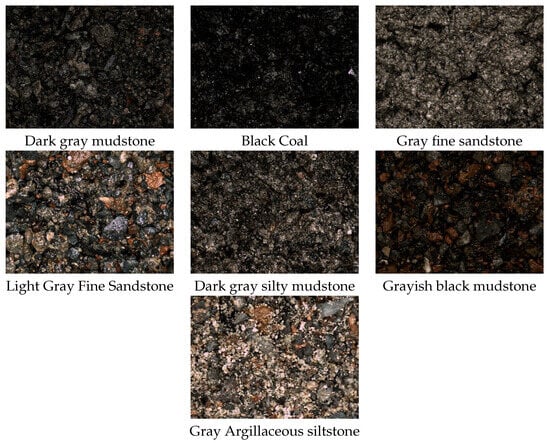
Figure 1. Rock images of seven categories.

This dataset was selected for the present study for two primary reasons: firstly, it has been extensively cited and validated within relevant fields, demonstrating robust reliability and widespread recognition; secondly, originating from an authoritative platform, it has undergone rigorous screening to ensure high quality, providing a solid foundation for research. Furthermore, the dataset encompasses a rich variety of categories with sufficient quantity. It includes 630 raw rock images across seven categories, such as black coal, gray fine sandstone, and dark gray silty mudstone. This scale and diversity fully meet the data requirements for lithological identification research, facilitating more comprehensive and precise analysis. Furthermore, from a geophysical perspective, it accurately reflects key characteristics of the research subjects and maintains close physical correlations with the scientific processes involved. This provides direct and meaningful input for subsequent studies based on machine learning and other methods, ensuring the scientific rigor and effectiveness of the research.

2.2. Multi-Scale Rock Image Feature Extraction Algorithm

Multi-angle rock feature extraction methods primarily analyze complex rock characteristics from three dimensions: rock grain size, image color features, and rock texture. By comprehensively extracting features from rock images across multiple dimensions, the internal information within them is maximized.

2.2.1. Color Feature Extraction

Color feature extraction is performed from three perspectives: First, indirectly extracting rock features through grayscale histograms; second, feature extraction based on the RGB three-primary-color model; third, feature extraction based on saturation, hue, and lightness within the HSV color space. Within each color space, the intensity values of its color channels are scaled from 0 to 255, where 0 represents the channel being off and 255 represents the channel being fully on.

• Gray Histogram Feature Extraction

Weight and sum the three channels of the rock image—B (blue), G (green), and R (red)—to obtain the grayscale value at each pixel point, then plot the grayscale histogram. Count the number of pixels corresponding to each grayscale level in the image to reflect the frequency of occurrence of different grayscale levels.

As shown in Figure 2, this essentially represents a statistical distribution chart of gray levels versus pixel counts. The gray histogram is segmented based on gray values, evenly dividing it into four intervals. Each interval contains 64 gray values:—Channel closed [0, 63]—Channel semi-closed [64, 127]—Channel semi-open [128, 191]—Channel open [192, 255] The number of pixels corresponding to each gray value interval is counted as one of four grayscale features, calculated as follows:

$$Gra{y}_i=\sum _{j=0}^{63}pixel{s}_{j+i\times 64},i\in [1,4]$$

(1)

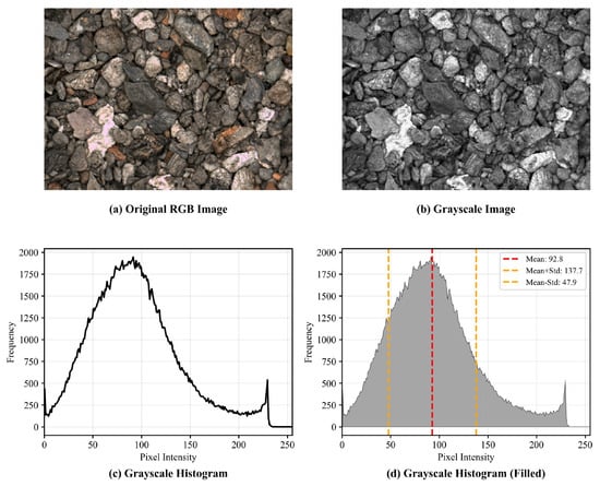
Figure 2. Gray-scale image and gray-scale color histogram.

Here, $Gra{y}_i$ represents the i-th feature extracted from the grayscale histogram, where j denotes the grayscale value in ascending order within the current interval, and j indicates the number of pixels with grayscale value j.

2.

RGB Channel Feature Extraction

Unlike gray histogram feature extraction, the RGB channels of a color image are separated, as shown in Figure 3:

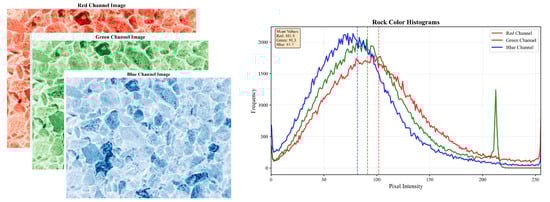
Figure 3. Rock images and color histograms under BGR channels.

Perform the same operation as gray histogram feature extraction—interval segmentation—on each channel, then calculate the number of pixels in each interval for each color channel. The formula is as follows:

$$x=\sum _{j=0}^{63}pixel{s}_{j+i\times 64},x\in [B_i,G_i,R_i]$$

(2)

where $B_i,G_i,R_i$ represent features extracted from the B, G, and R channels respectively; i denote interval features for the corresponding color channel, and $i\in [1,4]$.

3.

HSV Channel Feature Extraction

To achieve more comprehensive feature extraction, the HSV channel is processed similarly to the RGB channel. H represents the hue channel, S represents the saturation channel, and V represents the value channel. The formula is as follows:

$$y=\sum _{j=0}^{63}pixel{s}_{j+i\times 64},y\in [H_i,S_i,V_i]$$

(3)

2.2.2. Texture Feature Extraction

Rock texture characteristics represent a core concept in geology for describing the size, shape, arrangement, and geometric relationships of mineral or structural units across multiple scales. Their types exhibit significant differentiation based on rock genesis, such as crystalline textures in igneous rocks, layered textures in sedimentary rocks, and foliated textures in metamorphic rocks. As quantifiable key features, their parameters serve as vital references for rock identification, providing core support for rock classification, intelligent recognition, and subsequent mineral exploration.

For diverse rock images captured by industrial cameras, the visual texture is interpreted as the repetitive arrangement of tonal primitives [27,28]. The grayscale co-occurrence matrix is employed to extract texture features such as the spatial distance and variation amplitude between adjacent pixels in each rock image. To optimize texture information extraction, statistical processing is first applied, using the resulting second-order statistics as image feature parameters to describe texture characteristics. The texture feature extraction workflow is as follows:

(1)

Grayscale Conversion: Image texture arises from the regular distribution of grayscale values. Therefore, the average of the three RGB components is taken as the single-channel grayscale value, and the grayscale-converted image serves as the subject of study.

(2)

Gray-level reduction: The number of gray levels and image size determine the computational load of the gray-level co-occurrence matrix. In practice, the gray level is set to 4.

(3)

Set sliding window: The sliding window in the grayscale co-occurrence matrix functions similarly to a convolution kernel in convolutional neural networks. It calculates the pixel value of a given point by taking the weighted average of surrounding pixel values, where the weights are determined by the distance between pixels.

(4)

Select stride: Choose 8 rings with radii of 1, 3, 5, 7, 9, 11, 13, and 15 pixels from the center point. The distance between each ring is one pixel. As the distance increases by one pixel, the accuracy of the grayscale co-occurrence matrix decreases.

(5)

Calculate Statistics: Nine features are statistically analyzed: variance, homogeneity, contrast, mean, correlation dissimilarity, angular second moment, entropy, energy, and autocorrelation [16]. The primary statistics are entropy, angular second moment, and autocorrelation.

The Entropy statistic Ent is calculated as follows:

$$Ent=-\sum _{i=0}^{M-1}\sum _{j=0}^{N-1}f(i,j)lgf(i,j,d,\theta )$$

(4)

The Angular Second Moment (ASM) statistic formula is as follows:

$$ASM=\sum _{i=0}^{M-1}\sum _{j=0}^{N-1}f{(i,j,d,\theta )}^2$$

(5)

The autocorrelation statistic Cor is calculated as follows:

$$Cor=-\sum _{i=0}^{M-1}\sum _{j=0}^{N-1}{\displaystyle \frac{(i-\mu )(j-\mu )f{(i,j,d,\theta )}^2}{{\delta }^2}}$$

(6)

where: j denotes the mean gray value of the neighborhood, i represents the gray value of the pixel, $\theta$ indicates the direction angle, and d is the spatial distance.

2.2.3. Grain Size Feature Extraction

Grain size features reflect the structural characteristics of rock debris particles and serve as a crucial basis for rock classification [29,30]. Extracting grain size features imposes certain requirements on the image, such as high resolution, sharp edges, and rich texture details to ensure effective extraction and distinguishability of grain size features. Image-based grain size feature extraction methods primarily involve: preprocessing images to filter out extraneous rock features using Gaussian filtering; applying binarization and opening operations to highlight rock edge contours; calculating the area within these contours and deriving the equivalent average diameter of rock particles; and finally converting this into the mean equivalent diameter as a key feature metric representing the grain size characteristic for each rock category.

For data processed with the opening operation, contour detection is first performed to map the shape. The cv2.findContours() function in Python is used to locate contours, while cv2.drawContours() plots connected components. Contours are then counted, and all particles are identified through iteration. Based on these particles, the cv2.contourArea() function calculates the area enclosed by the shape contours.

Based on the Triassic stratum rock grain size analysis by Ye Hongfeng et al. and the research on the grain size distribution of loose rock in waste dumps by Xie Xuebin et al. [31,32], observation reveals that the coal in the dataset exhibits macroscopically crushed grain size, all below 50 mm. The grain sizes of various materials are summarized in Table 2:

Table 2. Rock particle size ranges.

Rock Type	Particle Size Range/mm
Coal	0~50
Mudstone	0~0.0039
Argillaceous Siltstone	0.0039~0.0625
Fine Sandstone	0.0625~0.25

Considering the conversion between the scale bar length under the microscope and pixel points during photography, a threshold small = 0.0039 is set here to filter out shape contours with area smaller than small, removing some impurity points. Then, the equivalent diameter is calculated for areas below the threshold. By traversing the image, the average equivalent diameter of all contours is computed, serving as the grain size feature data for a single image.

2.3. Correlation Analysis of Rock Image Features

To ensure the scientific validity and effectiveness of feature selection, this study systematically analyzed the correlations among the extracted 38-dimensional rock image features. Through Spearman’s correlation coefficient calculations and hierarchical clustering methods, we deeply explored the intrinsic relationships among color, texture, and grain size features, providing a theoretical basis for subsequent feature dimension reduction.

The Spearman rank correlation coefficient was employed to assess monotonic relationships among features, calculated as follows:

$$\rho =1-{\displaystyle \frac{6\sum d_i^2}{n(n^2-1)}}$$

(7)

where $d_i^2$ denotes the rank difference between feature values, and n represents the sample size. Compared to Pearson’s correlation coefficient, Spearman’s method imposes no strict requirements on data distribution and more accurately reflects nonlinear monotonic relationships.

Hierarchical clustering (Ward method) automatically grouped features with similar correlation patterns, generating a cluster heatmap that visually revealed the intrinsic structural relationships among features.

2.4. Rock Image Feature Dimension Reduction Algorithm Model

In machine learning, high-dimensional data often triggers the “curse of dimensionality,” making dimensionality reduction techniques indispensable. Traditional reduction methods lower data dimensions while preserving key information, laying the groundwork for subsequent analyses. Next, we leverage the Soft Voting ensemble approach to integrate three traditional dimensionality reduction methods—Lasso regularization, grey relational analysis, and variance filtering analysis—to enhance the robustness of feature reduction and achieve model simplification.

(1) LASSO (Least Absolute Shrinkage and Selection Operator) is a widely used linear model in regression analysis and feature selection [33]. Its core principle involves introducing an L1 norm penalty term to the least squares loss function. By constraining the sum of absolute model parameter values, it compresses some regression coefficients to zero, thereby achieving dual objectives: automatic feature selection and preventing overfitting. Specifically, the LASSO optimization objective function is expressed as follows:

$$\underset{\beta }{min}\left({\displaystyle \frac{1}{2n}}{\parallel y-X\beta \parallel }_2^2+\lambda {\parallel \beta \parallel }_1\right)$$

(8)

where $\lambda$ is the regularization strength hyperparameter and ${\parallel \beta \parallel }_1={\sum }_{j=1}^p\left|{\beta }_j\right|$ is the L1 norm. As $\lambda$ increases, more coefficients are forced to zero, leading to a sparser model. This characteristic makes LASSO particularly suitable for high-dimensional data scenarios. Its complexity is controlled by $\lambda$; a larger $\lambda$ imposes greater penalty on models with more variables in the linear model. Therefore, $\lambda$ serves as the weight for regularization. Variance filtering analysis removes features that fail to meet variance thresholds, so the threshold acts as the weight for variance filtering.

(2) For grey relational analysis, the tensor tendencies of each data group serve as the reference sequence Y, while the data features of each group form the comparison sequence $X_i$. Considering the differing magnitude scales of the factor sequences, dimensional normalization is applied by setting $\rho$ to 0.5, and calculate the gray-weighted correlation coefficient $r_i$ using the following formula:

$$r_i={\displaystyle \frac{1}{N}}\sum _{i=1}^n{\phi }_i\left(t\right),t=1,2,\dots ,n$$

(9)

${\phi }_i\left(t\right)$ where $r_i$ represents the correlation coefficient for the ith sample, and denotes the correlation weight from the voting method fusion. Soft Voting is then applied to further fuse the three selected features. Let $T_i$ be a 0–1 variable indicating whether a dimension reduction algorithm selected the feature. The final fusion results for each feature are as follows:

$${\mathrm{final}}_i=\lambda T_{i-\mathrm{lasso}}+r_i{T}_{i-\mathrm{gray}}+{\delta }_i{T}_{i-\mathrm{var}}$$

(10)

(3) Variance filtering is a common feature selection method whose core principle involves screening features based on their variance magnitude. Features with extremely low variance are typically considered to contain little useful information or may even represent noise. Therefore, features whose variance falls below a set threshold are eliminated to achieve dimensionality reduction, simplifying subsequent analysis and modeling processes.

$$\mathrm{Var}\left(x_i\right)={\displaystyle \frac{1}{n-1}}\sum _{j=1}^n{(x_{ij}-{\overline{x}}_i)}^2$$

(11)

The core of variance filtering lies in determining whether a feature’s variance meets the threshold requirement. Here, $\mathrm{Var}\left(x_i\right)$ represents the variance of feature $x_i$, measuring the dispersion of its values; $\theta$ is the predefined variance threshold used as the criterion for feature retention. When the variance of feature $x_i$ is less than the threshold $\theta$, it indicates that the feature exhibits minimal variation across samples and carries insufficient discriminative information, leading to its exclusion.

Voting is a voting machine incorporating ensemble thinking [34,35]. In Soft Voting, each base classifier first outputs probability values for each category rather than a single class label. The final prediction result is obtained by averaging these probabilities or through linear weighting. Integrating multiple dimension reduction algorithms to reduce data variance enhances the robustness of feature dimension reduction.

For the rock features extracted using the aforementioned methods, Soft Voting is applied for dimensionality reduction. Lasso regularization, grey relational analysis, and variance filtering analysis serve as the base reducers. Based on the correlation analysis results mentioned earlier, important rock features in high-dimensional rock images are retained, while noise and less significant features are removed, thereby achieving model simplification.

2.5. Base Learners

Within the ensemble learning framework, the Random Forest (RF) algorithm achieves prediction optimization by constructing a heterogeneous decision tree ensemble. Its core mechanism employs a dual randomization strategy: bootstrap sampling with replacement at the data level and subspace sampling at the feature dimension. This dual randomization effectively suppresses model overfitting tendencies, compensating for the overfitting risk of individual trees through the diversity of the ensemble. Notably, this method exhibits robustness to missing values and demonstrates strong adaptability in high-dimensional feature spaces and heterogeneous data scenarios. However, its model interpretability is constrained by the ensemble structure, and computational resource consumption exhibits exponential growth when handling large-scale training data.

The K-Nearest Neighbors (KNN) algorithm, based on spatial proximity principles, employs a non-parametric delayed learning mechanism in the image domain [36]. Its decision process relies on feature distance metrics such as Euclidean distance based on pixel values or cosine distance based on deep features between the target image and historical samples in the image library. By presetting the neighborhood parameter k, the algorithm performs majority voting or weighted voting decisions on the k nearest neighbor samples surrounding the target image. Since it does not require pre-training a fixed model, it is particularly suitable for scenarios such as dynamically expanding image libraries and real-time image retrieval. However, image data typically exhibits high dimensionality. Whether considering the expanded dimensions of the pixel matrix or the dimensions of deep features, the computational efficiency of distance calculations is significantly constrained by the curse of dimensionality. The sparsity of high-dimensional image feature spaces reduces the discriminative power of traditional distance metrics. In such cases, feature preprocessing techniques—such as image pixel normalization and CNN-based feature dimensionality reduction—alongside scaling methods like Z-score normalization are required to eliminate decision biases caused by pixel scale differences and redundant features.

The Naive Bayes classifier [37] within the probabilistic graphical model framework constructs a probabilistic inference system based on the assumption of feature conditional independence. By decomposing joint probability into a product of marginal probabilities, it significantly reduces computational complexity. In natural language processing, its polynomial variant demonstrates superior performance on bag-of-words models. However, in practical applications, latent correlations between features often distort probability estimates, particularly in long-tail data distributions where low-frequency features can easily trigger misclassifications.

Support Vector Machines [38] achieve pattern separation by constructing optimal classification hyperplanes, whose mathematical essence lies in solving constrained convex optimization problems. The introduction of kernel functions overcomes linear separability constraints by implicitly mapping the original space to a feature space with enhanced separability. This model exhibits outstanding generalization performance under small sample conditions, yet kernel function selection critically influences outcomes. Notably, its training time complexity grows cubically with the number of samples, creating a significant bottleneck in big data scenarios.

Sensitivity to noise varies significantly across algorithms: RF mitigates noise through ensemble strategies, while SVM remains highly sensitive to outliers near support vectors. Computational efficiency favors NBM, whose prediction process relies solely on probability multiplication. Regarding feature importance assessment, RF’s Gini importance metric provides an effective tool for interpretable machine learning. To more clearly present the contents of the above algorithms, they have been shown in Table 3. Therefore, by constructing the Stacking ensemble learning framework, which organically integrates the strengths of different algorithms, we achieve synergistic improvements in predictive performance while maintaining model diversity. This ultimately leads to significant enhancements in both model robustness and classification accuracy, avoiding the degradation of other performance metrics that often accompanies single-metric optimization.

Table 3. Advantages and Disadvantages of Base Learners in Image Analysis.

Algorithm	Advantages	Disadvantages
RF	High robustness and generalization, no feature selection, fast training, parallel processing.	Poor model interpretation, possible similar decision trees, high memory consumption.
KNN	Suitable for dynamic updating of training data, insensitive to outliers, robust, no need for complex training process.	Slow prediction, complex parameter tuning, performance degradation with high dimensional data.
NBM	Extremely fast training, suitable for high dimensional data, performs well for small data sizes, low computational complexity.	Difficult to ensure feature independence, sensitive to input data distribution, weak generalization ability.
SVM	Suitable for handling high-dimensional and non-linear data with good generalization ability.	Sensitive to noise, difficult selection of kernel function and parameters, slow training on large-scale data, high memory usage.

2.6. Stacking Model

The core scientific basis of Stacking models is the “error diversity” theory in ensemble learning. This theory states that when multiple base learners exhibit diversity and their errors are uncorrelated, an appropriate combination strategy can effectively reduce the overall model’s generalization error. Compared to existing single-model or simple model fusion approaches, this model innovates by employing a two-layer learning architecture: the first layer involves parallel learning by multiple heterogeneous base classifiers, while the second layer uses a meta-learner to perform optimal weighting of these base classifier outputs, achieving deeper model fusion.

Stacking ensemble learning steps: First, the original dataset is partitioned into multiple sub-datasets, serving as training sets for the base learners in Layer 1. Next, the training results from each base learner in Layer 1 are used as input data for Layer 2, where the meta-learner is trained. Finally, the meta-learner’s output is adopted as the final prediction result. The base layer of Stacking typically incorporates diverse learning algorithms, making Stacking ensembles inherently heterogeneous [39]. The algorithmic framework structure is illustrated in Figure 4 below:

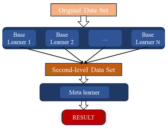
Figure 4. Stacking Integration Framework Diagram.

2.7. Parameter Optimization Algorithms

The Whale Optimization Algorithm (WOA) is a swarm intelligence optimization method inspired by the bubble net hunting behavior of humpback whales, demonstrating unique advantages in hyperparameter tuning tasks. This algorithm operates through the coordinated action of three core mechanisms: the Shrinking Envelope mechanism simulates a whale pod converging toward optimal solutions, enabling localized fine-grained search; the Spiral Update strategy balances global exploration and local exploitation via logarithmic spiral paths, effectively preventing premature convergence; while the Random Search mechanism enhances population diversity. The algorithm dynamically adapts to the complexity of high-dimensional parameter spaces by adaptively adjusting the probabilistic weights of these three behaviors. Its swarm intelligence characteristics enable WOA to concurrently optimize heterogeneous parameters like random forest depth and support vector machine kernel functions without requiring gradient information. The unique spiral equation design ensures robust global optimization capabilities and convergence accuracy while maintaining low computational cost. For base learner parameter optimization, this study employs the WOA algorithm to perform global hyperparameter tuning across four models: RF, KNN, LR, and NBM. Key optimized parameters include the maximum tree depth and node splitting criteria for RF, the number of nearest neighbors and distance metric for KNN, the regularization coefficient for LR, and the smoothing parameter for NBM. This optimization dynamically adjusts WOA’s search strategy to ensure parameter diversity while effectively suppressing overfitting, enabling each base learner to maximize its classification performance.

2.8. Stacking Model Based on Whale Optimization Algorithm

Previously, we discussed the base learners RF, KNN, NBM, and SVM, each with distinct strengths and weaknesses, alongside the whale optimization algorithm (WOA), which possesses outstanding optimization capabilities. The diversity of base learners is crucial for leveraging the advantages of the Stacking model, while WOA can effectively optimize the hyperparameters of base learners to enhance their performance. To fully integrate the strengths of base learners and optimize their performance using WOA, thereby constructing a superior ensemble model, we will now combine base learners with the Whale Optimization Algorithm to form a Whale Optimization Algorithm-based Stacking model. The specific steps are as follows.

(1)

Base Learner Selection: The first layer of training models forms the foundation of Stacking. The quality of submodels directly impacts Stacking accuracy. Therefore, four robust algorithmic models—RF, KNN, NBM, and SVM—are selected.

(2)

Concurrent Learning: Each of the four models (RF, KNN, NBM, SVM) undergoes 10-fold cross-validation. The Whale Optimization Algorithm (WOA) performs global optimization of key hyperparameters for these base learners, including maximum tree depth for RF, kernel type and penalty coefficient for SVM, to minimize overfitting.

(3)

Selection of Meta-Learners: The second layer fuses predictions from the first layer’s strong learners. Employing weak learners prevents overall model overfitting, with LR serving as the primary algorithm model.

(4)

Model Structure Determination: Based on the preceding steps, a two-layer algorithmic model is established. By integrating different algorithms into an ensemble network, the final rock intelligence recognition model structure is constructed using the Stacking ensemble method.

(5)

Derive Results: Use the training results from Step 2’s strong learners as input data for the meta-learner. Treat the rock categories in the original sample data as the output set. Train to obtain the weight assigned to each strong learner, then output the final prediction through a linear combination.

The rock category recognition algorithm based on Stacking integration employs deep feature extraction across three dimensions of rock images. It utilizes Voting to fuse three dimension-reduction methods—Lasso regularization, grey relational analysis, and variance filtering—and integrates five single algorithms (RF, KNN, LR, NBM, and SVM) into a rock intelligent recognition and classification model through the Stacking ensemble approach. The overall method flow is illustrated in Figure 5:

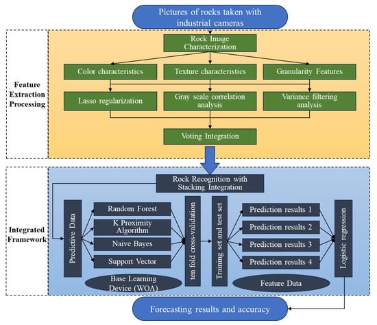
Figure 5. Flow of rock category recognition algorithm based on Stacking ensemble.

3. Experimental Simulation

3.1. Experimental Platform and Dataset Preprocessing

The experiment was conducted on a PC (CPU base speed: 2.2 GHz, 24 cores, 32 logical processors, 16.0GB RAM, NVIDIA GeForce RTX 4060 Laptop GPU) using the Jupyter Notebook 7.4.5 platform and Python 3.10 environment.

Preliminary analysis revealed significant class imbalance in the raw data, with certain rock types exhibiting substantially more samples than others. During the data preprocessing phase at, 315 clear images captured under white light conditions were selected for the dataset. This includes 289 close-range .bmp format images and 26 distant .jpg format images. To unify the image perspective, the .jpg images underwent border cropping to align their viewing angles with those of the .bmp images. To increase the sample size, images underwent multi-angle random rotation (90°, 180°, 270°), mirror flipping, Gaussian blurring, and translation transformations, supplemented by random cropping of the upper left, right, or lower corners. After these data augmentation processes, each category reached 100 samples, totaling 700 images with balanced category proportions. Detailed data information is shown in Table 4.

Table 4. Information table of rock image dataset.

Rock Type	Original Sample Size (Sheets)	Sample Size after Data Enhancement (Sheets)
Dark Gray Mudstone	30	100
Black Coal	21	100
Gray Fine Sandstone	18	100
Light Gray Fine Sandstone	85	100
Dark Gray Silty Mudstone	40	100
Grayish black mudstone	75	100
Gray Argillaceous Siltstone	46	100

Based on the Gaussian pyramid decomposition principle [40,41,42], the rock sample was progressively downsampled to a resolution of 28 × 28 pixels. The grayscale image generated at this scale offers dual advantages: it significantly reduces the computational complexity of subsequent feature calculations while preserving key characteristic information—such as rock texture orientation and mineral grain distribution—through a multi-resolution feature fusion mechanism, as shown in Figure 6.

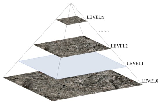
Figure 6. Schematic diagram of Gaussian pyramid.

Following Gaussian pyramid processing, the rock images undergo grayscale conversion, binarization, and morphological opening operations using Python programming. This yields an image dataset tailored for model training. For instance, as shown in Figure 7: (a) Grayscale conversion produces Figure 7d. (b) Binarization yields Figure 7e. (c) Opening operation results in Figure 7f.

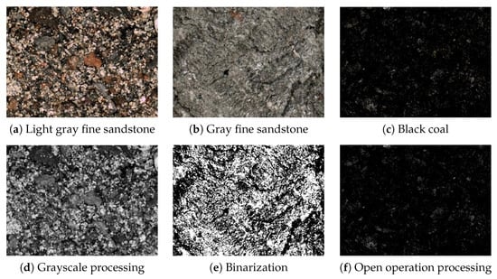
Figure 7. Display of some rock types after pretreatment.

3.2. Multi-Dimensional Feature Extraction

For the rock image data obtained through the aforementioned pretreatment, a multi-angle rock feature extraction method was employed to derive 38 rock features encompassing color, texture, and grain size. Specifically, 28 rock color features, 9 rock texture features, and 1 rock grain size feature were extracted.

3.2.1. Adding Color Features

For rock color characteristics, the brightness distribution across image channels was calculated using three color spaces: grayscale histogram, RGB, and HSV. All images in the dataset underwent traversal processing, with each rock image segmented uniformly into four features across its grayscale, RGB, and HSV channels, yielding a total of 28 feature data points. In Figure 8, the original image is divided into seven channels: grayscale, red, green, blue, hue, saturation, and brightness. Each channel contains four features, totalling 28 feature data points.

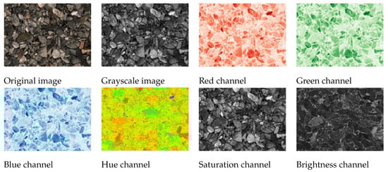
Figure 8. Characteristic decomposition of grayscale, RGB, and HSV channels of the rock image.

3.2.2. Adding Texture Features

For rock texture features, extraction is performed using the grayscale co-occurrence matrix. First, the grayscale co-occurrence matrix with a pixel distance of d = 1 (PPI) is computed along four directions: 0°, 45°, 90°, and 135°. Subsequently, nine feature parameters are extracted for each directional matrix: variance, homogeneity, contrast, mean, correlation/discrimination, angular second moment, entropy, energy, and autocorrelation. To eliminate directional sensitivity, the final value for each texture feature is calculated as the average of the four directional results, as shown in Figure 9.

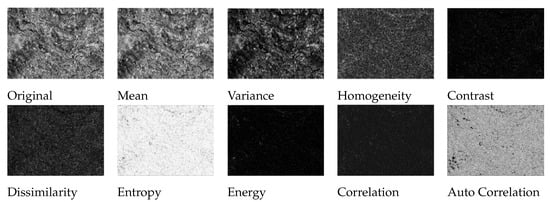
Figure 9. Rock texture characteristics.

3.2.3. Adding Graininess Features

For rock granularity features, the cv2.findContours() and cv2.contourArea() functions were used to draw contours around rock shapes and calculate the areas enclosed by these contours. By traversing the image, the equivalent diameters of all contours were computed and averaged. The resulting mean equivalent diameter served as the granularity feature data for each image, which was then input into the model’s training set. The granularity features for each image in the rock dataset are shown in Figure 10:

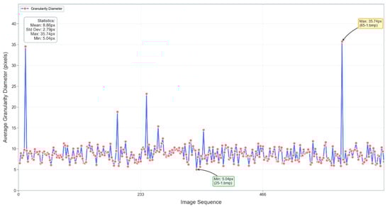
Figure 10. Distribution of particle size characteristics in the rock dataset.

3.3. Feature Correlation Validation

To validate the scientific validity of feature dimensionality reduction, a systematic correlation analysis was conducted on the 10 selected key features. Based on the comprehensive correlation heatmap shown in Figure 11, the correlation properties of the final 10 key features were critically examined, and the analysis results are shown in Table 5.

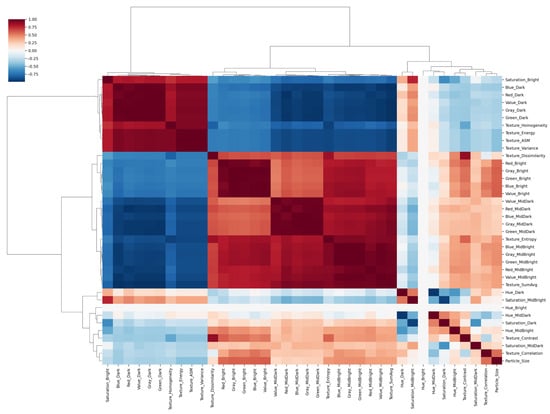
Figure 11. Hierarchical Clustering Correlation Heatmap of Rock Features.

Table 5. Feature Correlation Statistics After Dimension Reduction.

Statistical Metric	Value
Maximum Average Correlation	0.7410
Minimum Average Correlation	0.2149
Mean of Average Correlation	0.3371
Standard Deviation of Average Correlation	0.1498
Intra-group Average Correlation for Color Features	0.2661
Intra-group average correlation for texture features	0.3726

Analysis results indicate that the final 10 selected key features exhibit the following characteristics:

• We conducted a systematic correlation analysis on the final 10 selected features, calculating the average correlation between each feature and the others. The mean correlation among these 10 features was 0.3371, with a standard deviation of 0.1498. This maintains necessary discriminative information while effectively avoiding multicollinearity issues, ensuring the scientific rigor and validity of feature selection.
• Balanced Feature Types: Three color features (30%), six texture features (60%), and one grain size feature (10%). This distribution reflects the dominant role of texture features in rock classification while ensuring feature diversity.
• Distinct Clustering: The heatmap reveals features naturally grouping into three primary clusters corresponding to color, texture, and grain size features, validating the rationality of the feature extraction method.

3.4. Feature Dimension Reduction

After obtaining the 38 rock dataset features, three feature reduction algorithms—Lasso regularization, grey relational analysis, and variance filtering—were applied to calculate the contribution of each feature. This assessed feature importance and compared the stability and consistency among features across different reduction methods, with results shown in Figure 12.

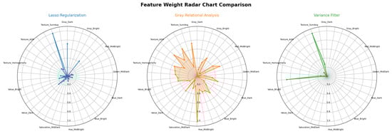
Figure 12. Contribution rate of each feature under Lasso regularization, grey correlation analysis, and variance filtering algorithms.

The evaluation results of the three dimensionality reduction methods were integrated using a voting approach to select the 10 most representative key features. The correlation among the filtered features was further analyzed to ensure that the selected features possess high discriminative power while effectively reducing redundancy, providing reliable inputs for subsequent modeling. The correlation of the filtered features is shown in Table 6:

Table 6. Characteristic Correlation Table.

Feature	Average Correlation	Feature	Average Correlation
Texture_SumAvg	0.7410	Texture_Entropy	0.2562
Texture_Contrast	0.4557	Texture_Dissimilarity	0.2547
Particle_Average_Granularity	0.3370	Gray_Bin1	0.2502
Hue_Bright	0.3333	Texture_ASM	0.2411
Texture_Variance	0.2869	Red_Bright	0.2149

3.5. Experimental Results and Analysis

The extracted features were fed into RF, KNN, SVM, and NBM models. The training and test sets were divided using 10-fold cross-validation [43]. Stacking was employed to integrate the five algorithms, forming a comparative experiment. The test accuracy rates for various rock types are shown in Table 7.

Table 7. Accuracy of various types of rocks under different algorithms.

	RF	KNN	NBM	SVM	Stacking
Dark Gray Mudstone	61.99%	64.53%	60.05%	70.99%	74.25%
Black Coal	91.11%	85.35%	91.91%	88.86%	97.16%
Gray Fine Sandstone	85.97%	84.97%	91.29%	91.24%	93.33%
Light Gray Fine Sandstone	78.68%	65.39%	73.65%	65.08%	82.65%
Dark Gray Silty Mudstone	74.86%	80.02%	73.15%	77.62%	81.21%
Grayish black mudstone	85.23%	79.67%	82.63%	82.06%	87.16%
Gray Argillaceous Siltstone	69.16%	77.45%	77.69%	73.42%	82.12%
Average	78.14%	76.77%	78.62%	78.47%	85.41%

Based on the test results, the rock classification performance achieved by the proposed Stacking ensemble algorithm in this paper is the most effective. Across different rock categories, its accuracy consistently outperforms that of any single stability classifier. By combining the five individual classifiers into a Stacking ensemble, the approach demonstrates superior classification accuracy and computational efficiency compared to the standalone algorithms. To further refine the Stacking ensemble structure, various structural combinations were explored, ultimately yielding a viable and stable reference solution.

As shown in Figure 13, a comparison of the average classification accuracies indicates that the optimal prediction performance was achieved when Random Forest (RF), K-Nearest Neighbor (KNN), Support Vector Machine (SVM), and Naïve Bayes (NBM) were employed as base learners, and Logistic Regression (LR) was used as the meta-learner in the second layer of the Stacking ensemble. The ensemble model attained an average accuracy of 85.41%, which exceeded the performance of any individual classifier. Among all lithological categories, black coal exhibited the highest classification accuracy, reaching 97.16%. Figure 14 illustrates the variation in the Stacking model’s accuracy with different feature retention ratios. The numbers labeled along the curve (3, 7, 10, 14, 17, 21, 24, 28, 31, and 38) represent the corresponding numbers of features retained at each ratio. It can be observed that as the feature retention ratio (i.e., the number of features used) changes, the model’s mean accuracy shows a fluctuating trend. The highest accuracy (Best = 0.8541) was obtained when ten features were retained. Overall, although minor fluctuations were observed, the variation range remained relatively limited, indicating that the model maintained stable performance. This finding further demonstrates that, compared with single-model training, the ensemble learning approach exhibits greater stability and robustness in its predictive capability.

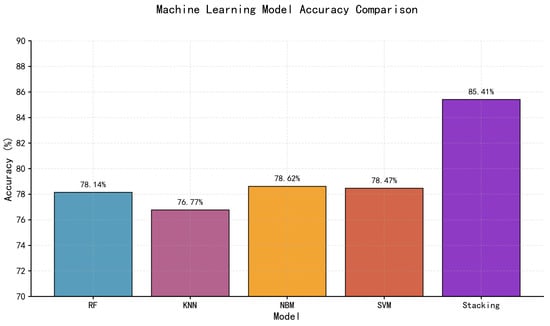
Figure 13. Comparison of results of each algorithm.

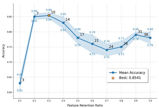
Figure 14. Variation of Stacking model accuracy with feature retention ratio.

3.6. Error and Analysis

To comprehensively evaluate the reliability of model classification, this study introduces four core metrics (accuracy, precision, recall, and F1 score) for error analysis, rather than relying solely on accuracy. The definitions of each metric are as follows:

$$\mathrm{Accuracy}={\displaystyle \frac{TP+TN}{TP+TN+FP+FN}}$$

(12)

where: $TP$ (True Positive) represents the number of samples that are actually positive and correctly predicted as positive; $TN$ (True Negative) represents the number of samples that are actually negative and correctly predicted as negative; $FP$ (False Positive) represents the number of samples that are actually negative but incorrectly predicted as positive; $FN$ (False Negative) represents the number of samples that are actually positive but incorrectly predicted as negative.

Precision calculates the proportion of truly positive samples among all samples predicted as positive by the model, and it can prevent false positive misjudgments. Its formula is as follows:

$$\mathrm{Precision}={\displaystyle \frac{TP}{TP+FP}}$$

(13)

Recall determines the percentage of positive samples correctly identified by the model among all actually positive samples, which can avoid false negative missed judgments. Its calculation formula is as follows:

$$\mathrm{Recall}={\displaystyle \frac{TP}{TP+FN}}$$

(14)

F1-Score is the harmonic mean of Precision and Recall. It can balance the performance of Precision and Recall and comprehensively reflect the overall stability of the classification model. The calculation formula is as follows:

$$\mathrm{F}1\text{-}\mathrm{Score}={\displaystyle \frac{2\times (\mathrm{Precision}\times \mathrm{Recall})}{\mathrm{Precision}+\mathrm{Recall}}}$$

(15)

Table 8 presents the 10-fold cross-validation results for key models (Stacking, NBM, RF) across evaluation metrics; Table 9 details the category-level F1 scores for the optimal model (Stacking).

Table 8. Average Performance of Key Models.

Model	Accuracy (%)	Precision (%)	Recall (%)	F1 (%)	Std. of F1 (%)
Stacking	85.41	84.92	85.17	85.04	1.28
NBM	78.62	78.05	78.23	78.14	1.76
SVM	78.47	77.91	78.08	77.99	1.82
RF	78.14	77.36	77.52	77.44	1.85
KNN	76.77	75.92	76.11	76.01	2.14

Table 9. Class-Level F1-Scores of the Stacking Model.

Rock Category	F1-Score (%)	Error Source Analysis
Dark Gray Mudstone	73.52	High similarity to dark gray silty mudstone
Black Coal	96.52	Distinct color/texture (low inter-class similarity)
Gray Fine Sandstone	92.48	Clear grain size features
Light Gray Fine Sandstone	82.48	Confusion with gray fine sandstone due to similar granularity and color
Dark Gray Silty Mudstone	81.06	Partial overlap with gray fine sandstone texture
Grayish black mudstone	86.98	Confusion with dark gray mudstone (similar color)
Gray Argillaceous Siltstone	82.24	Fine grain size leads to blurred texture features

In the error analysis of the rock classification task, there were significant differences in the performance of models across different categories and in model stability. Among them, black coal was representative of the high-performance category, achieving the highest F1-score (96.52%). This was due to its unique black appearance and crushed grain structure, which allowed it to be easily distinguished from other rock categories. In contrast, the high-error category was mainly dark gray mudstone, which had the lowest F1-score (73.52%). The core reason was that its color and texture characteristics were highly similar to those of dark gray silty mudstone, a situation that also conformed to the typical challenge of “high inter-class similarity” in small-sample fine classification tasks. From the perspective of model stability, the Stacking ensemble model performed the best, with an F1 standard deviation of only 1.28%. Compared with single models such as KNN (with an F1 standard deviation of 2.14%), it had stronger adaptability to sample variation and greater robustness, further verifying the advantage of the ensemble strategy in improving classification reliability.

3.7. Statistical Test

To verify whether the performance differences between models are statistically significant, this section first conducted a one-way ANOVA to test whether there are overall significant differences in the average F1 scores across all models; on this basis, the Tukey HSD post-hoc test (with a significance level of $\alpha =0.05$) was further used to identify which pairs of models have significant performance differences.

3.7.1. ANOVA Test Results

The ANOVA test was applied to the F1 scores of 5 models across 10 folds. The results are shown in Table 10:

Table 10. ANOVA Test Results for Model F1 Scores.

Test Metric	F-Statistic	p-Value	Significance ($\mathit{\alpha }$ = 0.05)	Interpretation
F1	42.87	<0.0001	Significant	Model performance differences are not random

The extremely small p-value (<0.0001) provides strong evidence against this null hypothesis. This indicates that at least two models have significantly different F1 scores. In other words, the observed differences in model performance, as reflected by the F1 scores, are not merely due to random chance but rather stem from genuine disparities in the models’ capabilities.

3.7.2. Tukey HSD Post-Hoc Test Results

The Tukey HSD test was used to compare pairwise model differences. Key results are shown in Table 11.

Table 11. Tukey HSD Test Results (Stacking vs. Other Models).

Model Pair	Mean Difference (F1)	95% Confidence Interval	p-Value	Significance
Stacking vs. NBM	6.84	[5.42, 8.26]	<0.0001	Significant
Stacking vs. SVM	7.08	[5.65, 8.51]	<0.0001	Significant
Stacking vs. RF	7.72	[6.30, 9.14]	<0.0001	Significant
Stacking vs. KNN	9.10	[7.67, 10.53]	<0.0001	Significant
NBM vs. SVM	0.24	[−1.18, 1.66]	0.893	Not Significant

The statistical test results conclusively demonstrate that the Stacking ensemble model achieved a significantly higher mean F1-score than all individual models (p < 0.0001). This finding corroborates its highest mean accuracy (85.41%) reported in Table 7, collectively validating the effectiveness of the ensemble learning strategy in this work.

4. Conclusions

This study focuses on the challenges in small-sample rock fine classification tasks, where the limited sample size easily leads to overfitting and the high similarity among rock categories increases the complexity of achieving fine classification accuracy. Under these circumstances, relying solely on a single algorithm becomes insufficient. To address this issue, this work employs a Stacking-based ensemble learning framework that integrates multiple classifiers, achieving significantly improved performance compared with individual models.

• Multi-Dimensional Feature Extraction Framework

A comprehensive feature extraction framework is developed by integrating multi-domain and multi-scale characteristic representations. Specifically, the statistical distributions of rock images across grayscale, RGB, and HSV color spaces are extracted, while gray-level co-occurrence matrices are employed to compute various texture descriptors. Additionally, morphological analysis combined with contour detection is applied to obtain grain-size–related structural features. These complementary descriptors constitute the initial feature set. Subsequently, feature correlation analysis and fusion-based dimensionality reduction techniques are used to select a compact subset of highly discriminative features, effectively enhancing rock feature representation and supporting high-precision classification.

2.

WOA-Optimized Stacking Ensemble Model

This study proposes a Stacking ensemble model optimized using the Whale Optimization Algorithm (WOA). WOA is applied to conduct hyperparameter optimization for heterogeneous base learners—including Random Forest, K-Nearest Neighbors, Support Vector Machine, and Naive Bayes—while Logistic Regression acts as the meta-classifier for prediction fusion. By fully exploiting the complementary strengths of different learning algorithms and enabling collaborative decision-making, the proposed framework significantly enhances classification robustness and generalization capability. Experimental results demonstrate that, for rock fine classification tasks with high inter-class similarity, the proposed method achieves an average classification accuracy of 85.41%, representing a 7.41% improvement over individual algorithms. These findings verify that Stacking ensemble learning can effectively improve fine classification performance under small-sample conditions.

However, some limitations still remain. The proposed model is trained and tested on a dataset comprising only 700 images, and the relatively small data scale may affect the generalization capability. Furthermore, the images were collected in non-ideal environments such as field or underground settings, where lighting variation and uneven resolution might distort color and texture features, introducing bias during feature extraction and consequently affecting classification accuracy. Future work will focus on expanding and augmenting the dataset and enhancing the robustness of feature extraction under complex environmental conditions.

References

- Zhou, L.M.; Wang, Y.Q. Challenges and strategies of deep resource exploration in China. J. Cent. South Univ. 2022, 29, 1021–1032. [Google Scholar]
- Zhang, L. Research and Application of Deep Learning-Based Rock Identification. Ph.D. Thesis, Guangxi Minzu University, Nanning, China, 2024. [Google Scholar] [CrossRef]
- Han, X. Research on Intelligent Identification of Rock Lithology Based on YOLOv7 and Swin Transformer. Ph.D. Thesis, East China University of Technology, Nanchang, China, 2024. [Google Scholar] [CrossRef]
- Jiang, Y.; Li, H.; Yan, X.; Zhang, T.; Wei, X.; Meng, C.; Chen, Q. Identification and prospecting application of wide-field electromagnetic method to deep pluton: Take the Longkou–Tudui gold deposit in Jiaodong as an example. J. Cent. South Univ. Sci. Technol. 2025, 56, 966–978. [Google Scholar]
- Ma, Q.; Ma, S.; Lei, Y. Geological Characteristics of Qinghai Province and Experience in Collecting Typical Geological Specimens. Geol. Rev. 2024, 70, 2031–2040. [Google Scholar] [CrossRef]
- Xiong, M.; Chen, L.; Chen, X.; Ji, Y.; Wu, P.; Hu, Y.; Wang, G.; Peng, H. Characteristics, genetic mechanism of marine shale laminae and its significance of shale gas accumulation. J. Cent. South Univ. Sci. Technol. 2022, 53, 3490–3508. [Google Scholar] [CrossRef]
- Zhu, S.; Yang, W.; Hou, G.; Lu, B.; Wei, S. An intelligent classification and identification method for rock thin sections. Acta Mineral. Sin. 2020, 40, 106. [Google Scholar]
- Zhang, Y.; Li, G.; Feng, J.; Li, M.; Su, T.; Wang, K. A Microscopic Mechanical Modeling Method for Rocks Based on the Multi-Crystal Discrete Element Method and Its Applications. In Proceedings of the 33rd National Natural Gas Academic Conference (2023) (01 Geological Exploration), Wuhan, China, 20–22 September 2023; China Petroleum Society Natural Gas Professional Committee, Southwest Petroleum University: Chengdu, China, 2023; pp. 664–677. [Google Scholar] [CrossRef]
- Zhang, Y.; Li, R.; Xi, S.; Yao, J.; Huang, H.; Zhao, B.; Wu, X.; Yang, L. Sedimentary environments and organic matter enrichment mechanism of Ordovician Wulalike Formation shale, western Ordos Basin. J. Cent. South Univ. Sci. Technol. 2022, 53, 3401–3417. [Google Scholar] [CrossRef]
- Xiao, Q.; Yuan, H.; Chen, C.; Li, Y.; Chen, C.; Zhang, X.; Kuang, M.; Xu, T.; Ye, Z.; Wang, T. Genesis Analysis of the Maokou Formation Dolomite in the Northern Sichuan Region: Evidence from Petrology, In-situ Geochemistry, and Chronology. Nat. Gas Geosci. 2024, 35, 1160–1186. [Google Scholar]
- Wang, C.; Liu, L.; Li, Q.; Meng, L.; Liu, C.; Zhang, Y.; Wang, J.; Yu, X.; Yan, K. Geochemical characteristics and genesis analysis of rock sources of brine-type lithium-potassium minerals in the Jitai Basin, Jiangxi Province. J. Petrol. Mineral. 2020, 39, 65–84. [Google Scholar]
- Meng, C.; Xue, J. X-ray fluorescence spectroscopy-X-ray diffraction study on the mineralogical characteristics of Helan stone rock in Ningxia. Rock Miner. Test. 2018, 37, 50–55. [Google Scholar] [CrossRef]
- Peng, Y.; Xue, H.; Zhao, Y.; Lan, Y.; Pan, L.; Zhang, C. Analysis of Factors Affecting the Image Quality of Scanning Electron Microscope Images of Rock Samples. Chin. J. Test. 2020, 46, 156–160. [Google Scholar]
- International Society FOR Rock Mechanics. Suggested Methods for Rock Identification; ISRM: Lisbon, Portugal, 2019. [Google Scholar]
- Wu, F.Q.; Zhang, R. Environmental constraints in deep mining: Global practices and China’s solutions. Nat. Sustain. 2023, 6, 158–170. [Google Scholar]
- Zhang, Y.; Li, M.; Han, S. Automatic lithology recognition and classification method based on deep learning of rock image. Acta Petrol. Sin. 2018, 34, 333–342. [Google Scholar]
- Bai, L.; Wei, X.; Liu, Y.; Wu, C.; Chen, L. Identification of Thin Section Images Based on the VGG Model. Geol. Bull. China 2019, 38, 2053–2058. [Google Scholar]
- Xu, Z.; Ma, W.; Lin, P.; Shi, H.; Liu, T.; Pan, D. Intelligent Rock Type Recognition Based on Image Transfer Learning. J. Appl. Basic Eng. Sci. 2021, 29, 1075–1092. [Google Scholar] [CrossRef]
- Cheng, G.; Li, B.; Wan, X.; Yao, W.; Wei, X. A Study on Rock Thin Section Image Classification Based on the SqueezeNet Convolutional Neural Network. J. Mineral. Petrol. 2021, 41, 94–101. [Google Scholar] [CrossRef]
- Zhang, C.; Yi, Y.; Zhou, W.; Qin, W.; Liu, W. Small-Sample Rock Classification Based on Deep Learning and Data Augmentation Techniques. Sci. Technol. Eng. 2022, 22, 14786–14794. [Google Scholar]
- Tan, Y.; Tian, M.; Xu, D.; Sheng, G.; Ma, K.; Qiu, Q.; Pan, S. Research on Rock Image Classification and Recognition Based on Xception Network. Geogr. Geoinf. Sci. 2022, 38, 17–22. [Google Scholar]
- Yuan, S. Study on the Lithology Identification Method of Rock Image Based on Deep Learning. Master’s Thesis, Northeast Petroleum University, Daqing, China, 2023. [Google Scholar]
- Ren, S.; Hu, Y.; He, W.; Gao, X.; Wan, T. Deep Learning-Based Microscopic Image Recognition of Sandstone Components. Sci. Technol. Eng. 2024, 24, 3727–3736. [Google Scholar]
- Guo, J. Research and Application of Rock Lithology Identification Algorithms Based on Fine-Grained Image Classification. Ph.D. Thesis, Southwest Petroleum University, Chengdu, China, 2024. [Google Scholar] [CrossRef]
- Zhou, C.; Liu, W.; Wu, T.; Li, A.; Han, X. Classification of rock thin section images based on a hybrid expert model. J. Jilin Univ. Sci. Ed. 2024, 62, 905–914. [Google Scholar] [CrossRef]
- He, L.; Zhou, Y.; Zhang, C. Application of Deep Learning-Based Object Segmentation in Intelligent Rock Recognition. Bull. Mineral. Petrol. Geochem. 2025, 44, 525–541+452. [Google Scholar] [CrossRef]
- Li, M.; Fu, J.; Zhang, Y.; Liu, C. Intelligent recognition and analysis method for lithology classification by coupling rock image and hammering audio. J. Rock Mech. Eng. 2020, 39, 996–1004. [Google Scholar] [CrossRef]
- Fan, P. A Study on Cluster Analysis Based on Rock Image Features. Ph.D. Thesis, Xi’an Petroleum University, Xi’an, China, 2018. [Google Scholar]
- Liu, C.; Xu, Q.; Shi, B.; Gu, Y. Digital Image Recognition Methods and Applications for Rock Particles and Pore Systems. Chin. J. Geotech. Eng. 2018, 40, 925–931. [Google Scholar]
- Du, S.; Zhang, W.; Teng, Y.; Guo, Q. Analysis of Grain Size Characteristics in Clastic Sandstones of the Zhuhai Formation in the Baiyun Depression. J. Xi’an Univ. Arts Sci. Nat. Sci. Ed. 2022, 25, 116–121. [Google Scholar]
- Ye, H.; Gao, X.; Fu, N.; Wang, F.; Wang, J. Analysis of rock grain size and discussion of sedimentary environment in the Triassic strata of the Qumalai area, Qinghai Province. Gansu Geol. 2022, 31, 17–23. [Google Scholar]
- Xie, X.; Pan, C. Fractal characteristics of particle size distribution and shear strength of bulk rock in waste dump. Geotech. Mech. 2004, 25, 287–291. [Google Scholar] [CrossRef]
- Zhang, L.; Wei, X.; Lu, J.; Pan, J. Lasso regression: From interpretation to prediction. Adv. Psychol. Sci. 2020, 28, 1777–1791. [Google Scholar] [CrossRef]
- Zhang, D.; Liu, Y.; Zhang, W.; Shen, F.; Yang, J. Detection of fake reviews based on heterogeneous ensemble learning. J. Shandong Univ. Eng. Ed. 2020, 50, 1–9. [Google Scholar]
- Zheng, Y.; Wang, Z. Research on Credit Bond Default Early Warning Based on Multi-Objective Optimization Weighted Soft Voting Integration Algorithm. Mod. Electron. Technol. 2024, 47, 43–48. [Google Scholar] [CrossRef]
- Li, E.; Zhang, B.; Jia, B. A Two-Stage Multidimensional Classification Method Combining KNN Feature Enhancement and Mutual Information Feature Selection. Computer Engineering and Applications, pp. 1–14. Available online: http://kns.cnki.net/kcms/detail/11.2127.tp.20250225.1800.023.html (accessed on 23 May 2025).
- Ou, G.; He, Y.; Zhang, M.; Huang, Z.; Fournier-Viger, P. Risk Minimization Weighted NBM Classifier. Comput. Sci. 2025, 52, 137–151. [Google Scholar]
- Liu, D.; Sun, J.; Zhang, L.; Yang, Y.; Zhang, L.; Zhang, Z. Division method of tensile and shear crack and its application in sandstone rockburst precursor. J. Cent. South Univ. Sci. Technol. 2023, 54, 1153–1167. [Google Scholar] [CrossRef]
- Shi, J.; Zhang, J. Load forecasting method based on multi-model fusion Stacking integrated learning. Chin. J. Electr. Eng. 2019, 39, 4032–4042. [Google Scholar] [CrossRef]
- Lv, B.; Li, L.; Li, J.; Guo, T. Hidden target detection based on Gaussian pyramid and bilateral filtering. Sci. Technol. Eng. 2021, 21, 7649–7656. [Google Scholar]
- Lin, C.; Zhou, H.; Chen, W. Retinex image enhancement algorithm based on Gaussian pyramid transformation with bilateral filtering. Laser Optoelectron. Prog. 2020, 57, 209–215. [Google Scholar]
- Li, R.; Li, Y. Multi-scale feature identification of PCB bare board defects. China Test. 2024, 50, 181–190+200. [Google Scholar]
- Li, Z.; Cao, B.; Peng, D.; You, Q.; Miu, X.; Chen, Z. Inverse Inversion of Nuclear Accident Source Terms Based on Bayesian Neural Networks. Nucl. Electron. Detect. Technol. 2025, 45, 780–787. [Google Scholar] [CrossRef]
Disclaimer/Publisher’s Note: The statements, opinions and data contained in all publications are solely those of the individual author(s) and contributor(s) and not of MDPI and/or the editor(s). MDPI and/or the editor(s) disclaim responsibility for any injury to people or property resulting from any ideas, methods, instructions or products referred to in the content. |
© 2025 by the authors. Licensee MDPI, Basel, Switzerland. This article is an open access article distributed under the terms and conditions of the Creative Commons Attribution (CC BY) license (https://creativecommons.org/licenses/by/4.0/).