A Hybrid GRU-MHSAM-ResNet Model for Short-Term Power Load Forecasting

Abstract

Reliable load forecasting is crucial for ensuring optimal dispatch, grid security, and cost efficiency. To address limitations in prediction accuracy and generalization, this paper proposes a hybrid model, GRU-MHSAM-ResNet, which integrates a gated recurrent unit (GRU), multi-head self-attention (MHSAM), and a residual network (ResNet)block. Firstly, GRU is employed as a deep temporal encoder to extract features from historical load data, offering a simpler structure than long short-term memory (LSTM). Then, the MHSAM is used to generate adaptive representations by weighting input features, thereby strengthening the key features. Finally, the features are processed by fully connected layers, while a ResNet block is added to mitigate gradient vanishing and explosion, thus improving prediction accuracy. The experimental results on actual load datasets from systems in China, Australia, and Malaysia demonstrate that the proposed GRU-MHSAM-ResNet model exhibits superior predictive accuracy to compared models, including the CBR model and the LSTM-ResNet model. On the three datasets, the proposed model achieved a mean absolute percentage error (MAPE) of 1.65% (China), 5.52% (Australia), and 1.57% (Malaysia), representing a significant improvement over the other models. Furthermore, in five repeated experiments on the Malaysian dataset, it exhibited lower error fluctuation and greater result stability compared to the benchmark LSTM-ResNet model. Therefore, the proposed model provides a new forecasting method for power system dispatch, exhibiting high accuracy and generalization ability.

1. Introduction

Modern power systems are challenged by the expansion of smart grids [1] and the large-scale integration [2] of renewable resources [3]. These include accommodating rising electricity demand, the effective utilization of renewable energy, and the need for operational efficiency. The secure, reliable, and cost-effective operation of power systems has become a key objective in global energy strategies [4]. In this context, load forecasting serves not only as a fundamental tool for optimizing generation scheduling and reducing operational costs, but also as a critical technology for enabling source–grid–load–storage coordination and maintaining grid security and stability [5].

Short-term load forecasting is essential for maintaining the supply–demand balance in power systems. It also supports real-time dispatch and market operations [6,7]. Its accuracy is affected by socioeconomic factors such as population distribution and industrial energy efficiency. It is also influenced by environmental conditions, especially weather [8]. Among these factors, temporal features have a significant impact on forecasting performance. Incorporating temporal features during model training can enhance prediction accuracy [9].

In recent years, machine learning techniques, particularly deep learning, have opened new avenues for short-term load forecasting. Models such as extreme gradient boosting (XGBoost) and recurrent neural networks (RNNs) have been shown to capture key patterns within time series data. However, these methods still face considerable challenges in real-world applications. For instance, a single model struggles to simultaneously capture the diverse temporal dependencies and non-linear characteristics inherent in load data.

The increasing complexity of modern power system operations has imposed more stringent requirements on short-term load forecasting. To address this challenge, both academia and industry have pursued improvements in accuracy and robustness of forecasting models. Statistical approaches have long served as a foundation for load forecasting, with classical models include the autoregressive moving average (ARMA) [10], autoregressive integrated moving average (ARIMA) [11], simple exponential smoothing [12], and the Holt–Winters (HW) exponential smoothing method [13]. However, a significant limitation of these methods is their strict assumption of data stationarity.

Tree-based models, particularly random forests (RF), are widely used for short-term load forecasting. These models are valued for their robustness and ability to capture complex non-linear patterns. Ref. [14] proposed a hybrid prophet-RF model for medium-term load forecasting, which leverages the RF algorithm to capture non-linear relationships that complement the linear trend-fitting capabilities of the prophet model. Ref. [15] proposed a data-driven framework that utilized an XGBoost model, which demonstrated the highest accuracy in forecasting photovoltaic power generation based on time-ahead weather data. Ref. [16] proposed a hybrid forecasting model for short-term wind-power forecasting, consisting of an improved superb fairy-wren optimization algorithm combined with a support vector machine (ISFOA-SVM). In this model, the ISFOA is utilized to automatically optimize the key hyperparameters of the SVM, thereby addressing its parameter sensitivity and enhancing prediction accuracy. Ref. [17] proposed an XGBoost-based model for very short-term load forecasting, which improves accuracy by incorporating day-ahead load forecast results to provide trend information and a load variation feature to capture residual, rapid fluctuations. Ref. [18] proposed a hybrid framework for short-term power outage forecasting, which first employs a relevance vector machine (RVM) to capture complex non-linear relationships, then uses a wavelet transform (WT) and adaptive boosting (AdaBoost)with regression and threshold to model the RVM’s residuals, and finally stacks the individual predictions with a RF meta-model to enhance accuracy.

Building on advances in deep learning approaches, this method has been increasingly used in load forecasting. Among them, RNNs are particularly notable for their application to time series problems. Variants such as long short-term memory (LSTM) and gated recurrent units (GRU) incorporate gating mechanisms to capture long-range dependencies in series data. By this architecture, the vanishing and exploding gradient issues inherent to conventional RNNs are mitigated, and prediction accuracy is consequently improved [19,20].

The highly complex and non-linear characteristics of load data, conventional RNN models often fail to achieve desirable predictive accuracy. Consequently, researchers have increasingly adopted RNN variants to further enhance predictive performance. Ref. [21] proposed a Bayesian-optimized LSTM neural network to accurately forecast the net load in fault-affected areas, providing precise input for the subsequent fault recovery strategy. Ref. [22] proposed a LSTM-based model for very short-term load forecasting, which enhances the input sequences by integrating pseudo-trend components generated from a Kalman filter-based predictor to improve forecasting performance.

However, the predictive accuracy of any single model remains inherently limited. Therefore, approaches based on hybrid models are considered a promising strategy for further enhancing forecasting accuracy. Ref. [23] proposed a Bayesian-optimized model for power load forecasting, which first employs a graph convolutional network to capture spatial correlation features, then uses a bidirectional long short-term memory network (BiLSTM) to capture long-term temporal dependencies, and finally integrates the predictions through a Bayesian-optimized AdaBoost framework that dynamically adjusts base learner weights. Ref. [24] proposed a hybrid LSTM-XGBoost framework for smart-grid load forecasting. The LSTM network first extracts temporal dependencies, and the XGBoost model is then trained on the LSTM outputs to refine predictions, resulting in higher accuracy and robustness on 15 min Elia grid data. Ref. [25] proposed a hybrid model for energy consumption forecasting, which first employs LSTM to extract high-level latent features from historical data, and then utilizes these features as input to an XGBoost model to generate the final forecasting results.

As research has progressed, it has been observed that hybrid models may still exhibit performance limitations, with forecasting capabilities across different application scenarios. In comparison, hybrid models augmented with attention mechanisms are more effective at extracting salient features from load data. Ref. [26] proposed a hybrid model for quarter-hourly power load forecasting. The model first applies a combined data processing approach that integrates complete ensemble empirical mode decomposition with adaptive noise, k-means clustering, and variational mode decomposition to extract feature components from historical load data. It then utilizes a convolutional neural network (CNN) and a BiLSTM network to learn spatiotemporal features. Finally, an attention mechanism is employed to enhance key information for improved prediction accuracy. Ref. [27] proposed a composite model that combines CNN, LSTM, and attention mechanism. The framework is designed to first extract significant features using the CNN, then capture their temporal relationships using the LSTM, and finally, assign greater importance to critical information through the attention mechanism. Ref. [28] proposed a load forecasting model that first partitions load nodes into spatiotemporally homogeneous sub-regions using shape dynamic time warping and spectral clustering. A local spatiotemporal graph convolutional network is then applied to each sub-region, while a cross-regional attention mechanism enables the collaborative fusion of global features.

In summary, based on the reviewed literature, although machine learning and deep learning techniques are widely applied in load forecasting, several challenges remain:

(1)

A key limitation of existing hybrid models is that the importance of input features is not evaluated dynamically. Consequently, important features may be overlooked under different datasets. This reduces their ability to generalize across different datasets and application conditions.

(2)

Higher model complexity may improve accuracy. However, simply stacking modules often does not lead to a stable or generalizable system. Many such models fail to balance accuracy and generalization. Therefore, it remains a challenge to design a hybrid model that can effectively meet different forecasting needs.

To address these challenges, this paper proposes a hybrid model that integrates a gated recurrent unit (GRU) network, a multi-head self-attention mechanism (MHSAM), and a residual network (ResNet) block, hereafter referred to as GRU-MHSAM-ResNet. This hybrid model is designed to further improve the prediction accuracy of short-term load forecasting:

(1)

A deep temporal encoder, composed of stacked GRU layers, is employed to effectively capture the complex non-linear temporal dependencies inherent in the load data.

(2)

The vector output by the GRU encoder after processing historical load data is concatenated with the load from the previous hour ($L_{t-1}$), hour type ($H$), and week type ($W$) for forecast time t. The resulting concatenated vector is then passed into a MHSAM. In this module, MHSAM is used in parallel to focus on different parts of the input. This structure helps capture complex dependencies within the merged features better than simpler attention mechanisms. As a result, this allows the model to differentially weight features when constructing representations of the input.

(3)

The skip connections of ResNet block ensure that the model can converge stably and achieve improved prediction accuracy, even as network depth increases. This architecture allows the model to safely increase its depth, ensuring stable convergence and enhancing its capacity to extract complex features from the data.

Finally, the proposed GRU-MHSAM-ResNet model is compared with the CBR model proposed in Ref. [29] and the LSTM-ResNet model presented in Ref. [30]. Its superior predictive accuracy and generalization ability are further validated on the China and New South Wales (Australia) datasets.

The remainder of this paper is organized as follows: Section 2 introduces the structure and training method of the proposed GRU-MHSAM-ResNet model. Section 3 explains the data preprocessing, data normalization, and evaluation metrics. Section 4 describes the experimental setup and results; it includes model settings and a comparison of different models on two datasets. Finally, the conclusions are presented in Section 5. The limitations of the model are discussed, and future research directions are outlined.

2. Method

2.1. Model Framework

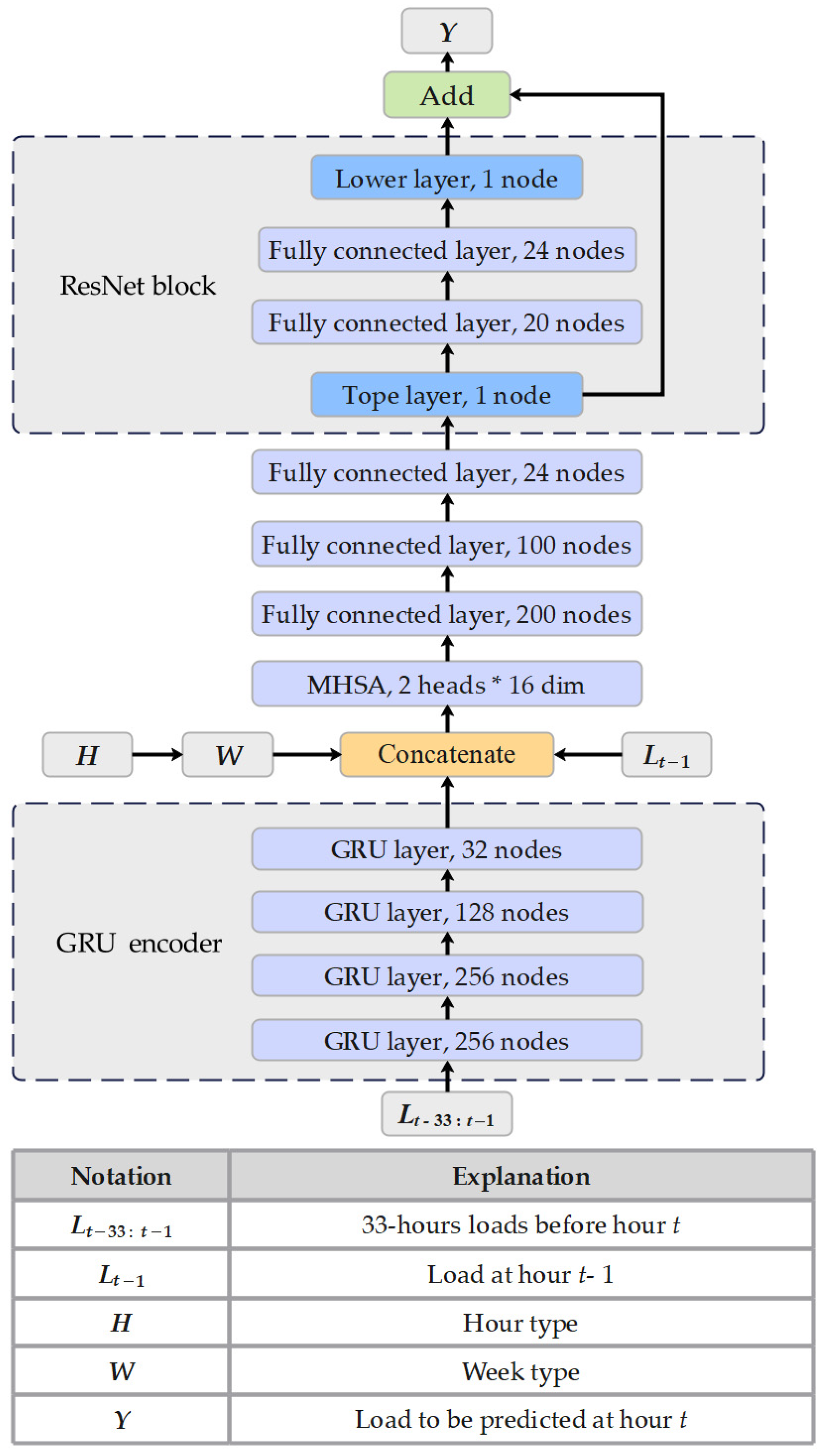
A framework for short-term load forecasting is proposed, in which a model based on GRU, MHSAM, and ResNet is introduced, as shown in Figure 1. In this model, temporal features are extracted from historical load data and concatenated with other inputs ($L_{t-1}$, $H$, $W$) to learn the relationships between input and output variables, leading to high forecasting accuracy. The forecasting process includes four stages: data preprocessing, extraction of historical load features, key information extraction, and finally, feature integration and prediction.

Figure 1. Framework of GRU-MHSAM-ResNet model.

(1)

Data preprocessing: Historical load data is processed using a sliding window method, and temporal information is extracted from it. This step prepares the input and output datasets required for model training and forms the foundation for the training phase.

(2)

Historical load feature extraction: The preprocessed historical load data is input into a GRU encoder. Taking advantage of the GRU’s ability to capture temporal patterns, deeper features in the historical data are extracted. The encoder’s final hidden state is used as the output.

(3)

Key information extraction: The features extracted by GRU encoder are concatenated with temporal information from the preprocessing stage and the load from the previous hour. This concatenated feature is then passed into the MHSAM. This mechanism is used to adaptively learn internal relationships within the input.

(4)

Feature integration and prediction: The output from the MHSAM is passed into a fully connected network for further processing. At the end of this network, a ResNet block composed of fully connected layers and a skip connection is incorporated to generate the final prediction results.

2.2. GRU Model

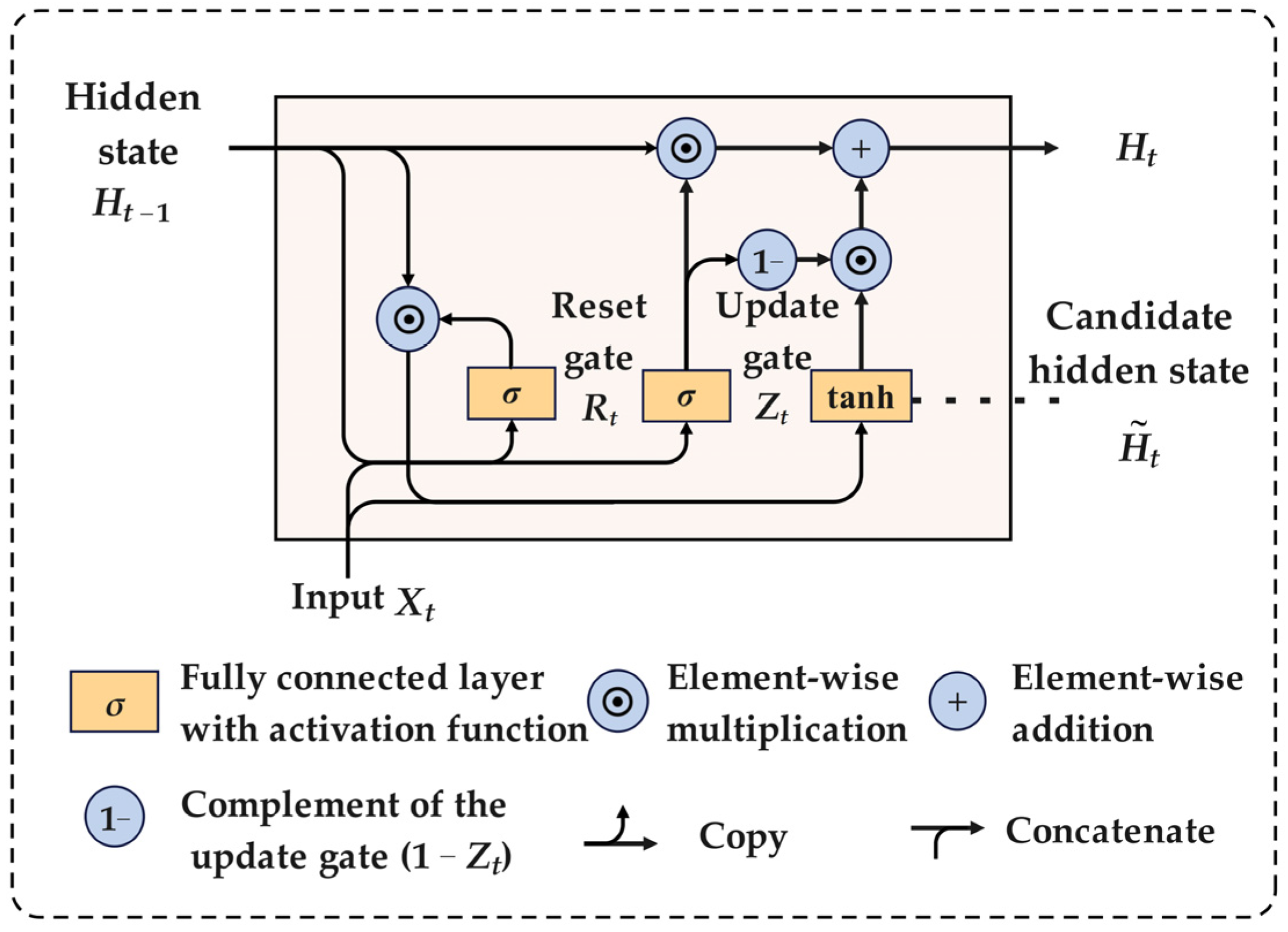
The gated recurrent unit (GRU) is an efficient variant of the RNN, specifically designed for time series tasks. It simplifies the control of information flow using two gates: an update gate and a reset gate. At each time step, the proportion of past information retained is governed by the update gate. In contrast, the amount of information discarded is dictated by the reset gate. Compared to the LSTM, the GRU has a simpler structure with fewer parameters, yet often achieves similar performance across many tasks [31]. This design makes the GRU more robust when handling long sequences and more adaptable in resource-constrained environments. The GRU structure is shown in Figure 2.

Figure 2. GRU structure.

The inputs for both the update and reset gates are derived from the state of the previous time step, $H_t$ and the current input $X_t$. The gate outputs are produced within the interval [0, 1] by a fully connected layer followed by a sigmoid function. Long-term dependencies are captured by the update gate, while the short-term patterns are captured by the reset gate [32]. The internal structure of the GRU is defined by Equations (1)–(4).

$$Z_t=\sigma \left(W_z\times \left[H_{t-1},X_t\right]+b_z\right)$$

(1)

$$R_t=\sigma \left(W_r\times \left[H_{t-1},X_t\right]+b_r\right)$$

(2)

$${\tilde{H}}_t=\tanh \left(W_h\times \left[R_t\ast H_{t-1},X_t\right]+b_h\right)$$

(3)

$$H_t=Z_t\ast H_{t-1}+\left(1-Z_t\right)\ast {\tilde{H}}_t$$

(4)

where $Z_t$ represents the update gate. $R_t$ represents the reset gate. ${\tilde{H}}_t$ represents the candidate hidden state at time step $t$. $H_t$ represents the final hidden state at time step. $H_{t-1}$ represents the hidden state at time step $t-1$. $W$ and $b$ represent the weights and biases, and the symbol $\ast$ represents the element-wise multiplication. The sigmoid and tanh functions are defined by Equations (5) and (6).

$$\sigma \left(x\right)={\displaystyle \frac{1}{1-e^{-x}}}$$

(5)

$$\tanh ={\displaystyle \frac{e^x-e^{-x}}{e^x+e^{-x}}}$$

(6)

2.3. Multi-Head Self-Attention Module

Self-attention, a variant of the attention mechanism, allows the model to weigh the importance of different parts of an input sequence in parallel. For each element in the sequence, attention scores are computed based on its relevance to all other elements. This produces a contextual representation that captures the importance of each element within the entire sequence.

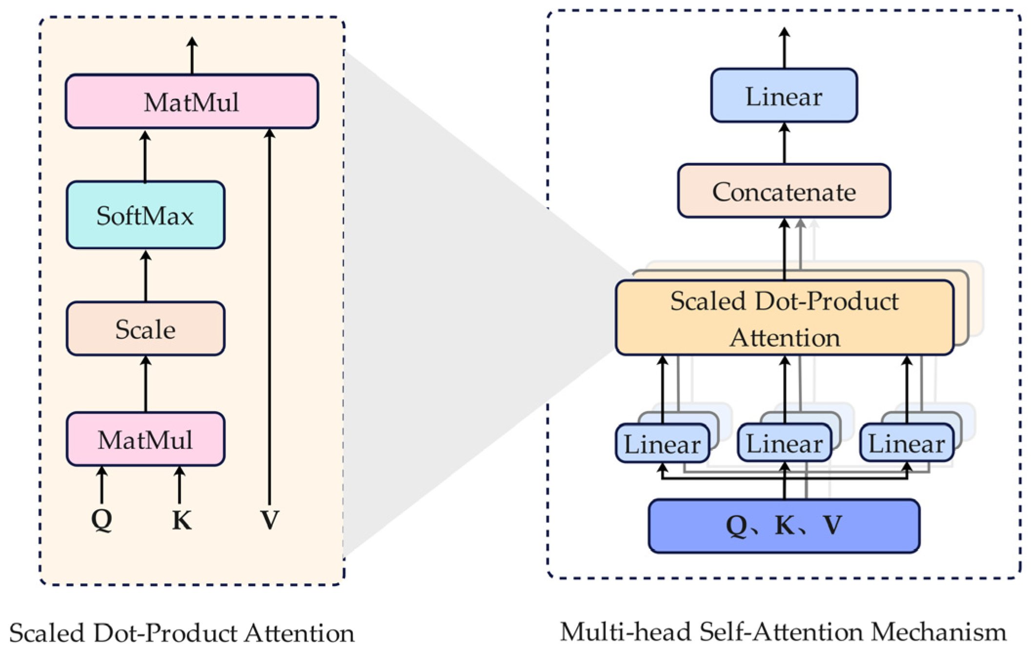
The multi-head self-attention mechanism (MHSAM) is an extension of the self-attention technique by running multiple self-attention heads in parallel. Each head applies a different linear transformation, allowing it to independently focus on different features of the input. The structure of MHSAM is defined by Equations (7)–(9) and shown in Figure 3.

$$\mathrm{Attention}\left(Q,K,V\right)=\mathrm{Softmax}\left({\displaystyle \frac{Q{K}^T}{\sqrt{d_K}}}\right)\times V$$

(7)

$${\mathrm{Attention}}_i\left(X\right)=\mathrm{Attention}\left(Q{W}_i^Q,K{W}_i^K,V{W}_i^V\right)$$

(8)

$$\mathrm{MultiHead}\left(X\right)=\mathrm{Concat}\left({\mathrm{Attention}}_1\left(X\right),\dots ,{\mathrm{Attention}}_h\left(X\right)\right)W_0$$

(9)

where $Q,K,V$ represents the query, key, and value matrices. $d_K$ represents the dimension of the query and key. $W_i^Q$, $W_i^K$, $W_i^V$ and $W_0$ are the learnable weight matrices. $\mathrm{Concat}\left(·\right)$ is the concatenate operation. $h$ is the number of the self-attention mechanisms, called head number.

Figure 3. MHSAM structure.

2.4. ResNet Block

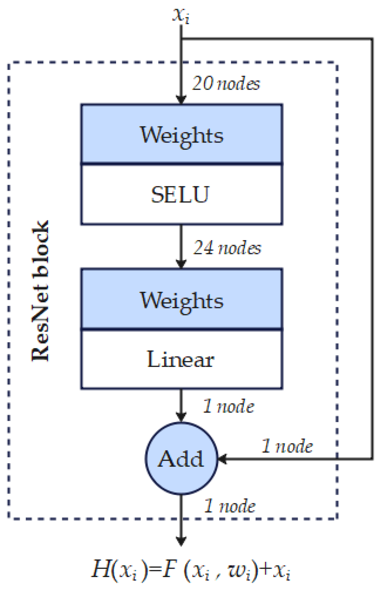
A residual network (ResNet) is a deep neural network architecture designed to address vanishing gradient and performance degradation problems that often occur during the training of deep models. Its core concept involves using skip connections to pass input information directly to deeper layers. This design improves both training efficiency and model performance and has shown strong results in computer vision tasks such as image classification and object detection. The structure of the ResNet block is shown in Figure 4.

Figure 4. ResNet block structure.

In recent years, ResNet has been applied more widely, architectures based on fully connected layers have also shown strong performance in load forecasting [33]. As shown in Figure 4, a basic residual block consists of two fully connected layers and an addition layer. The first fully connected layer has 20 nodes and uses the SELU activation function, while the second has 24 nodes with a linear activation, which is then projected to a final single-node output. This ensures that both the residual output $F\left(x_i,w_i\right)$ and the input $x_i$ are single-node vectors, allowing element-wise addition to be performed. The output of the ResNet block is defined by Equation (10).

$$H\left(x_i\right)=F\left(x_i,w_i\right)+x_i$$

(10)

where $x_i$ and $w_i$ represent the input and weights of the i-th ResNet block. $F\left(x_i,w_i\right)$ is the residual function. $H\left(x_i\right)$ represents the output of the ResNet block.

2.5. Training Details

This paper adopts a method that combines offline and online learning strategies to improve the model’s adaptability and accuracy in short-term load forecasting.

(1)

Offline learning phase: In the initial stage of forecasting, the model is trained on historical data, including both training and validation sets. This phase helps the model learn typical load patterns from a large dataset and build a solid performance for future predictions. Offline learning uses batch training to gradually optimize model weights, ensuring certain predictive abilities when facing new data.

(2)

Online learning phase: After offline training is completed, the model enters the online learning phase. For each test sample, once a prediction is made, its input and true output are added to the historical dataset to form an expanded training set. One epoch of training is then performed on this updated set to fine-tune the model weights established during offline training. This helps the model adapt to new data and learn recent trends in power load changes.

(3)

Prediction and update cycle: After each prediction, the model’s weights are updated using the online learning method. The updated model is then used to forecast the next data points in the test set. This cycle repeats continuously, allowing the model to improve over time and gradually increase its prediction accuracy.

3. Data Preprocessing and Evaluation Metrics

3.1. Data Preprocessing

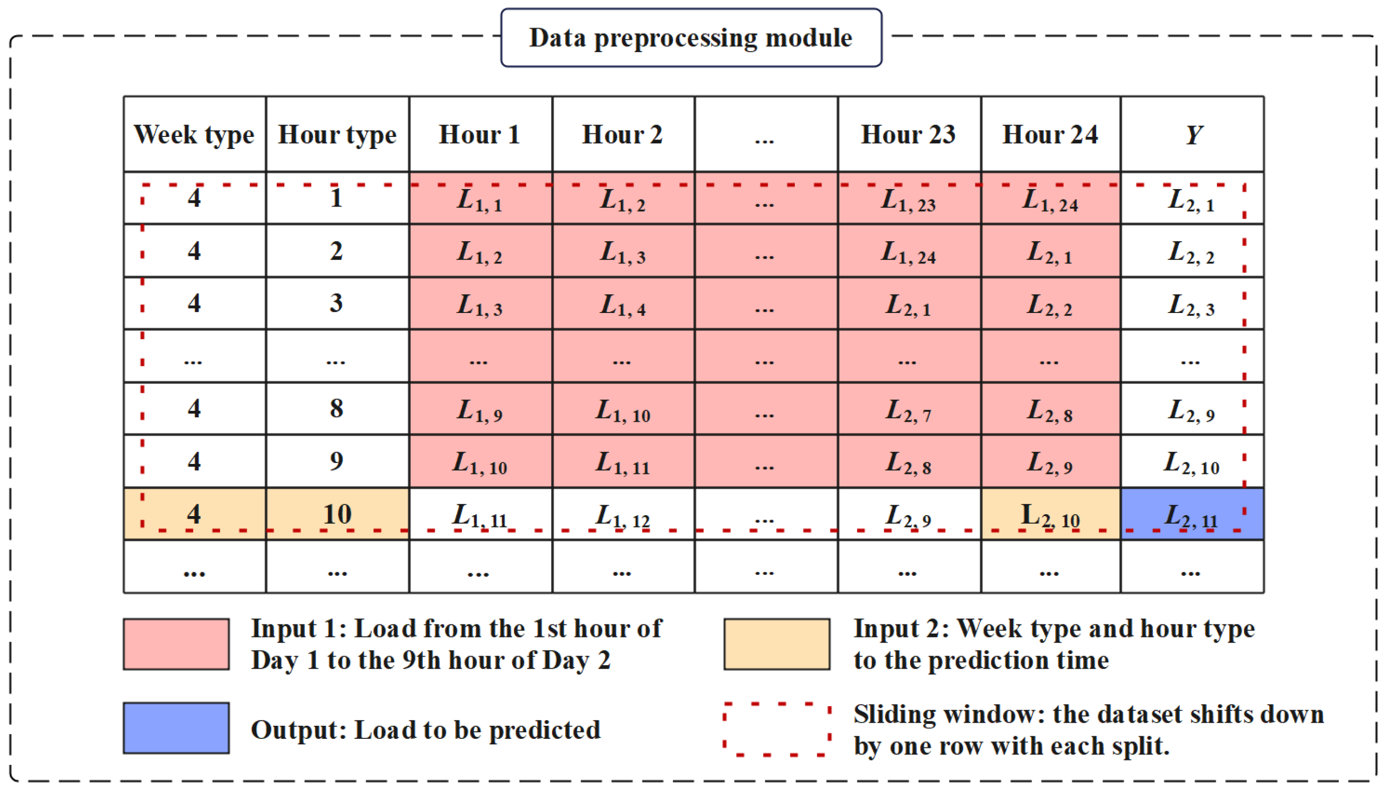
The dataset used in this experiment consists of hourly load data spanning one year. The division of inputs and outputs is shown in Figure 5, with details as follows:

Figure 5. Data preprocessing module.

(1)

33 h loads before hour t: The loads from the 33 h preceding the forecast hour t serve as the first part of the input. A sliding partition method is applied: each row of load data covers a continuous 24 h span. For example, the first row contains 24 load values from 00:00 to 24:00 on 1 January; the second row contains 24 values from 01:00 on 1 January to 01:00 on 2 January, and so forth. The first 10 rows constructed in this way are used as the first input for prediction model.

(2)

Load at hour t − 1: The load at the hour immediately before hour t serves as the second input for prediction model.

(3)

Hour type and week type: The hour information and the week information corresponding to hour t serve as the third input for prediction model.

(4)

Output: The load at hour t is defined as the model output.

3.2. Data Normalization

Datasets in load forecasting usually contain features such as temporal information, meteorological information, and historical load. These features often have different scales and numerical ranges. In deep learning models, such scale differences may cause the model to rely too heavily on features with larger values, increasing complexity and even leading to overfitting. Therefore, data normalization is adopted as a key preprocessing step to map features into a uniform range. In this paper, the Min-Max normalization method is used to scale features into the range [0, 1]. Compared with other methods, Min-Max normalization is simpler and preserves the relative distribution of the data, making it well-suited to the training needs of deep learning models. The normalization and denormalization processes are defined in Equations (11) and (12).

$$x^{\prime }={\displaystyle \frac{x-x_{\min }}{x_{\max }-x_{\min }}}$$

(11)

$$x=x^{\prime }\times \left(x_{\max }-x_{\min }\right)+x_{\min }$$

(12)

where $x$ represents the original data. $x^{\prime }$ represents the normalized value. $x_{\min }$ and $x_{\max }$ are the minimum and maximum values of the load data, respectively.

3.3. Evaluation Metrics

To compare the prediction accuracy of different models, three error metrics are used: total energy error (TEE), mean absolute percentage error (MAPE), and mean forecast error (MFE). These metrics are defined by Equations (13)–(15).

$${\epsilon }_{\mathrm{TEE}}={\displaystyle \sum _{t=1}^T\left|y_t-{\widehat{y}}_t\right|}$$

(13)

$${\epsilon }_{\mathrm{MAPE}}={\displaystyle \frac{1}{T}}{\displaystyle \sum _{t=1}^T\left|\frac{y_t-{\widehat{y}}_t}{y_t}\right|\times 100\%}$$

(14)

$${\epsilon }_{\mathrm{MFE}}=\sqrt{{\displaystyle \frac{1}{T}}{\displaystyle \sum _{t=1}^T{\left(\frac{y_t-{\widehat{y}}_t}{y_t}\right)}^2}}\times 100\%$$

(15)

where $y_t$ represents the actual load at hour $t$. ${\widehat{y}}_t$ represents the predicted load at the same hour, and $T$ represents the total duration.

The TEE measures the total error over the entire forecast period and is calculated by summing the absolute differences between predicted and actual values. MAPE gauges prediction accuracy by averaging the absolute percentage errors. MFE reveals the overall forecast bias by calculating the average difference between predicted and actual values.

4. Case Study

4.1. Experiment Environment and Training Hyperparameter Selection

The experiments were executed on a workstation equipped with an Intel Ultra 7 265K CPU and an NVIDIA GeForce RTX 4060 Ti GPU. The model was implemented in Python 3.9 using the TensorFlow 2.10.0 framework.

The proposed model parameters include the settings of GRU layers, fully connected layers, and residual block, as well as training epochs, batch size, optimizer, and loss function. The model’s hyperparameters and key settings are summarized in Table 1.

Table 1. Hyperparameters and basic settings of the model.

Parameter	Value
Nodes in the GRU layers	256/256/128/32
Number of heads in MHSAM	2
Dimension per head in MHSAM	16
Nodes in fully connected layers	200/100/24/1
Nodes in the ResNet block	20/24/1
Epoch	500
Batch size	128
Optimizer	Adam
Loss	MSE

4.2. Design of Comparison Models

To evaluate the performance of the proposed model, a comparative analysis was conducted. This analysis involved three distinct experimental groups. The models from Ref. [29] (Group 1) and Ref. [30] (Group 2) were used as compared models for comparison against the GRU-MHSAM-ResNet model proposed in this paper (Group 3). The composition of the experimental groups is described as follows:

Group (1): CBR model [29]. Feature extraction is performed by a one-dimensional convolutional neural network (1D CNN). A parallel forecasting structure is then employed to predict the base and elastic components of the load separately. An improved ResNet is included to improve generalization and mitigate the vanishing gradient problem. Since the original model used only an offline learning strategy, it will be evaluated in the experiment without online learning. This allows for an accurate assessment of its original performance.

Group (2): Region-holiday split/region split-LSTM model [30]. This method improves forecasting accuracy by predicting the load for each sub-region and accounting for holiday effects. It uses a hybrid model combining LSTM and a residual network. This model adopted both offline and online learning strategies to adapt to new data.

Group (3): GRU-MHSAM-ResNet (proposed model). The proposed model uses a GRU encoder to extract temporal features from historical load data. A MHSAM is used to generate adaptive representations by weighting input features. It also adopts a hybrid offline–online learning strategy.

4.3. Case 1: China System Analysis

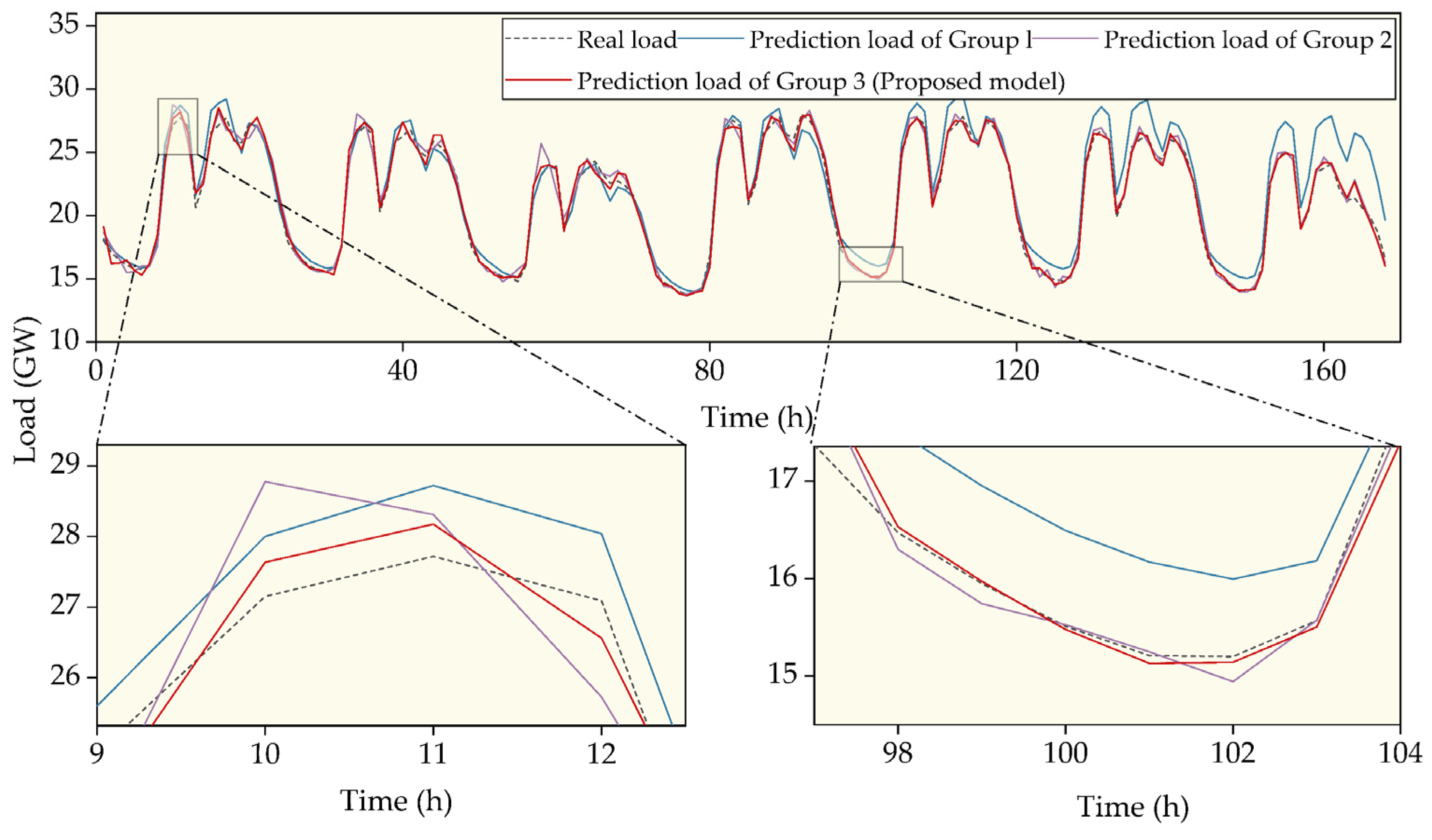
The models were tested on the China system load dataset, spanning from 1 January 2009, to 31 December 2009. The dataset was recorded at an hourly resolution, totaling 8760 data points. The data captures the region’s electric load fluctuations over the year. The forecasting results of three models on this dataset (test set) are shown in Figure 6 and Table 2.

Figure 6. Load forecasting results on the China dataset.

Table 2. Forecasting results for the three methods on the China dataset.

Model	TEE (GWh)	MAPE (%)	MFE (%)
Group (1)	168.9	4.74	6.68
Group (2)	77.83	2.06	2.73
Group (3)	59.41	1.65	2.23

As shown in Figure 6, Group 1 and Group 2 models perform poorly in overall fit and in capturing peak and valley values, indicating larger forecasting deviations. The error analysis in Table 2 further confirms this, showing that their error metrics are significantly higher than those of Group 3. In contrast, the best fitting performance was achieved by the proposed model (Group 3). The peaks and valleys of the load data were accurately captured. Furthermore, its prediction curve was closest to the actual data. After de-normalizing the predicted values, the error metrics in Table 2 were computed by comparing them with the actual data.

4.4. Case 2: New South Wales, Australia System Analysis

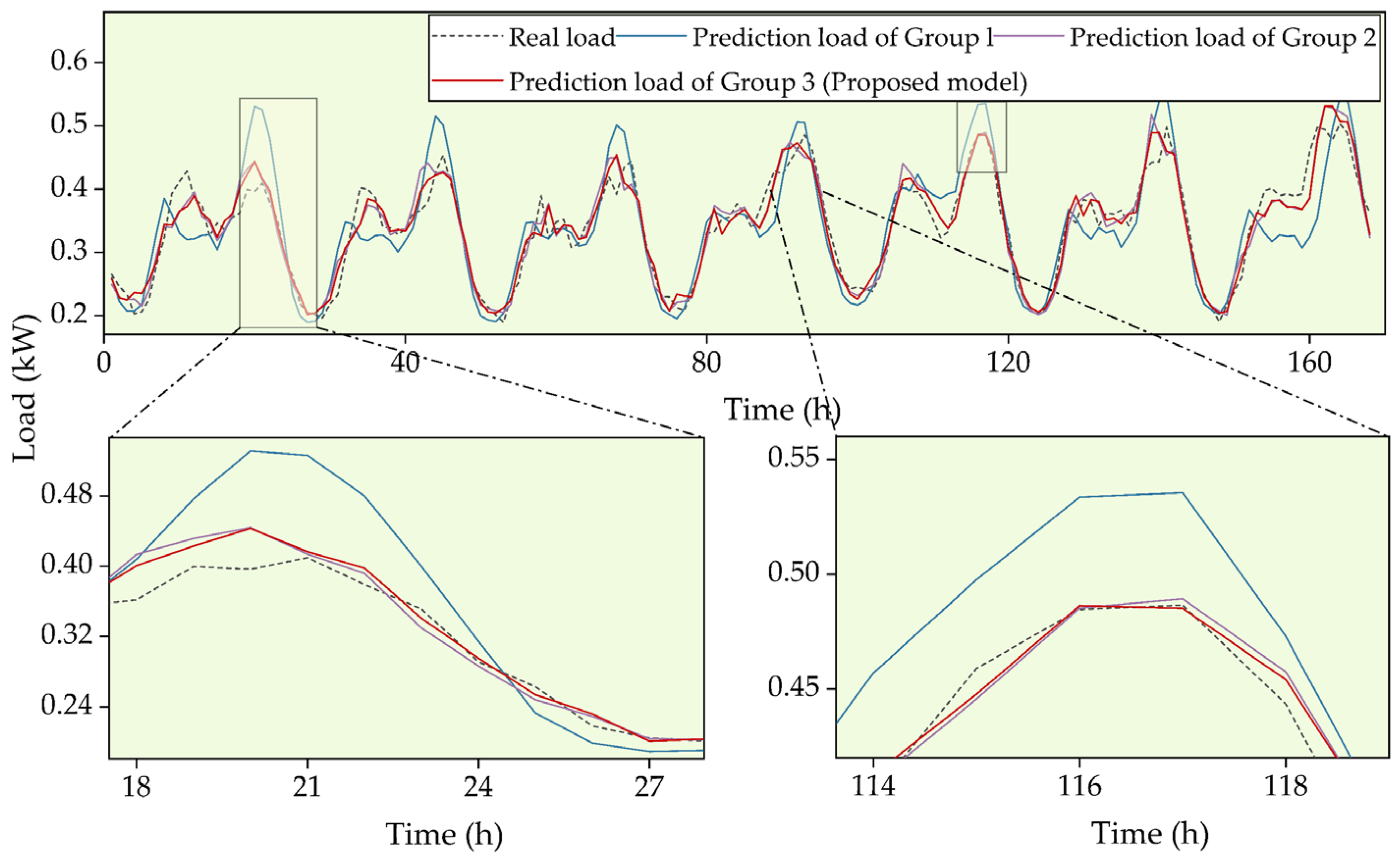
The models were tested on the New South Wales, Australia system load dataset, spanning from 1 January 2013 to 31 December 2013. The forecasting results of three models on this dataset (test set) are shown in Figure 7 and Table 3.

Figure 7. Load forecasting results on the Australian dataset.

Table 3. Forecasting results for the three methods on the Australia dataset.

Model	TEE (kWh)	MAPE (%)	MFE (%)
Group (1)	5.72	9.62	12.02
Group (2)	3.34	5.75	7.25
Group (3)	3.18	5.52	7.03

As shown in Figure 7, the predictions from the Group 1 and Group 2 models align well with the actual data during stable periods but fail to capture trends during periods of complex fluctuations. In contrast, the proposed model (Group 3) closely matches the actual data. These observations are further supported by the error analysis in Table 3, which shows that the lowest error metrics were achieved by the proposed model. This confirms its superior forecasting performance. Error metrics were calculated as in Section 4.3.

4.5. Case 3: Malaysia System Analysis

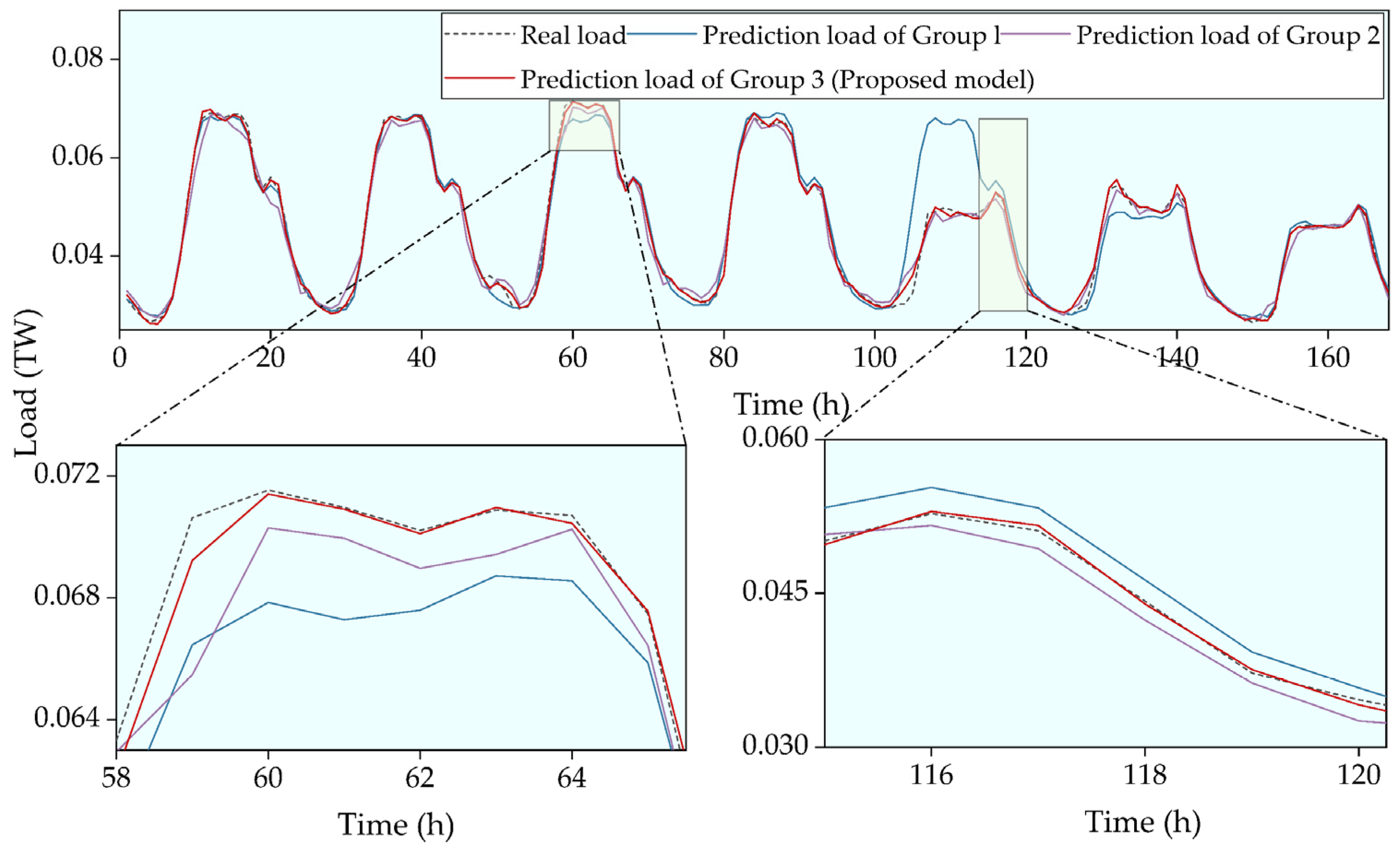
The models were tested on the Malaysia system load dataset, spanning from 1 January 2009 to 31 December 2010. The forecasting results of three models on this dataset (a portion of the test set) are shown in Figure 8 and Table 4.

Figure 8. Load forecasting results on the Malaysia dataset.

Table 4. Forecasting results for the three methods on the Malaysia dataset.

Model	TEE (TWh)	MAPE (%)	MFE (%)
Group (1)	2.80	4.28	9.03
Group (2)	1.14	1.83	2.87
Group (3)	0.99	1.57	2.37

As shown in Figure 8, all three models capture the overall load trends, but the proposed model (Group 3) provides significantly better accuracy, especially during periods of load fluctuation. This is further confirmed by the quantitative results in Table 4, where Group 3 achieves the lowest TEE, MAPE, and MFE values, demonstrating its superior prediction performance compared to Group 1 and Group 2. Error metrics were calculated as in Section 4.3.

4.6. Accuracy and Stability Analysis

The proposed GRU-MHSAM-ResNet model is a refined version of the LSTM-ResNet model described in Ref. [30]. As shown in Table 5, higher prediction accuracy and more stable error performance are achieved by the proposed model. With the same ResNet component, the use of GRU instead of LSTM improves computational efficiency and reduces model complexity. In addition, the MHSAM is used to generate adaptive representations by weighting input features. Through this mechanism, relevant internal patterns are better captured, which leads to improved accuracy and stability.

Table 5. Comparison of MAPE results from five runs between LSTM-ResNet and GRU-MHSAM-ResNet on the Malaysia dataset.

Model	Result of Train 1	Result of Train 2	Result of Train 3	Result of Train 4	Result of Train 5	Mean Result
LSTM- ResNet	1.76	1.88	1.78	1.72	2.02	1.83
GRU-MHSAM-ResNet	1.57	1.59	1.58	1.57	1.56	1.57

5. Conclusions

To enhance the accuracy of short-term load forecasting in power systems, this paper introduces a novel hybrid model: GRU-MHSAM-ResNet. This synergistic design leverages the complementary strengths of sequential modeling, context-aware feature weighting, and deep representation refinement, thereby achieving superior predictive performance.

The proposed model was validated on three actual load datasets from China, Australia, and Malaysia. Compared to the CBR model in Ref. [29], the proposed model reduced TEE by 64.8% (China), 44.4% (Australia), and 64.6% (Malaysia). MAPE was reduced by 65.19% (China), 42.62% (Australia), and 63.3% (Malaysia), and MFE was reduced by 66.6% (China), 41.5% (Australia), and 73.8% (Malaysia). Compared to the LSTM-ResNet model in Ref. [30], the proposed model reduced TEE by 23.6% (China), 4.7% (Australia), and 13.2% (Malaysia), reduced MAPE by 19.9% (China), 4.0% (Australia), and 14.2% (Malaysia), and reduced MFE by 18.3% (China), 3% (Australia), and 17.4% (Malaysia). These results confirm the model’s high prediction accuracy and practical application potential.

While the proposed model shows strong performance, its limitations also present directions for future research. For example, incorporating a broader set of meteorological features and modeling sub-regional dynamics could enhance the model’s ability to capture complex load patterns. Furthermore, exploring explicit sequence decomposition might allow the model’s non-linear modeling capabilities to focus on the most difficult residual components, potentially improving both performance and interpretability. Finally, as quantifying prediction uncertainty is critical for risk management, extending the model into a probabilistic forecasting framework and adopting comprehensive metrics such as CRPS remains a vital direction.

References

1. Dowejko, J.; Jaworski, J. Beyond traditional grid: A novel quantitative framework for assessing automation’s impact on system average interruption duration index and system average interruption frequency index. Energies 2025, 18, 2671. [Google Scholar] [CrossRef]
2. Kumar, G.V.B.; Sarojini, R.K.; Palanisamy, K.; Padmanaban, S.; Holm-Nielsen, J.B. Large scale renewable energy integration: Issues and solutions. Energies 2019, 12, 1996. [Google Scholar] [CrossRef]
3. Yang, H.; Chen, Q.; Tang, K.; Zhang, D.; Shen, Y. Flexibility aggregation and cooperative scheduling for distributed resources using a virtual battery equivalence technique. Energy 2025, 334, 137770. [Google Scholar] [CrossRef]
4. Yang, H.; Chen, Q.; Liu, Y.; Ma, Y.; Zhang, D. Demand response strategy of user-side energy storage system and its application to reliability improvement. J. Energy Storage 2024, 92, 112150. [Google Scholar] [CrossRef]
5. Shah, S.A.H.; Ahmed, U.; Bilal, M.; Khan, A.R.; Razzaq, S.; Aziz, I.; Mahmood, A. Improved electric load forecasting using quantile long short-term memory network with dual attention mechanism. Energy Rep. 2025, 13, 2343–2353. [Google Scholar] [CrossRef]
6. Ahmad, N.; Ghadi, Y.; Adnan, M.; Ali, M. Load forecasting techniques for power system: Research challenges and survey. IEEE Access 2022, 10, 71054–71090. [Google Scholar] [CrossRef]
7. Boroojeni, K.G.; Amini, M.H.; Bahrami, S.; Iyengar, S.S.; Sarwat, A.I.; Karabasoglu, O. A novel multi-time-scale modeling for electric power demand forecasting: From short-term to medium-term horizon. Electr. Pow. Syst. Res. 2017, 142, 58–73. [Google Scholar] [CrossRef]
8. Huang, R.; Zhu, L.; Gao, F.; Wang, Y.; Yang, Y.; Xiong, X. Short-term power load forecasting method based on variational modal decomposition for convolutional long-short-term memory network. Mod. Electr. Power 2024, 41, 97–105. [Google Scholar] [CrossRef]
9. Rubasinghe, O.; Zhang, X.; Chau, T.K.; Chow, Y.H.; Fernando, T.; Lu, H.H. A novel sequence to sequence data modelling based CNN-LSTM algorithm for three years ahead monthly peak load forecasting. IEEE Trans. Power Syst. 2024, 39, 1932–1947. [Google Scholar] [CrossRef]
10. Yang, Z.; Ce, L.; Lian, L. Electricity price forecasting by a hybrid model, combining wavelet transform, ARMA and kernel-based extreme learning machine methods. Appl. Energy 2017, 190, 291–305. [Google Scholar] [CrossRef]
11. Tarmanini, C.; Sarma, N.; Gezegin, C.; Ozgonenel, O. Short term load forecasting based on ARIMA and ANN approaches. Energy Rep. 2023, 9, 550–557. [Google Scholar] [CrossRef]
12. Rao, C.; Zhang, Y.; Wen, J.; Xiao, X.; Goh, M. Energy demand forecasting in China: A support vector regression-compositional data second exponential smoothing model. Energy 2023, 263, 125955. [Google Scholar] [CrossRef]
13. Liu, C.; Sun, B.; Zhang, C.; Li, F. A hybrid prediction model for residential electricity consumption using holt-winters and extreme learning machine. Appl. Energy 2020, 275, 115383. [Google Scholar] [CrossRef]
14. Cheng, S.; Shi, J.; Cheng, Q.; Zhou, X.; Zeng, S. Hybrid model for medium-term load forecasting in urban power grids. Energies 2025, 18, 4378. [Google Scholar] [CrossRef]
15. Minhas, D.M.; Usman, M.; Raja, I.B.; Wakeel, A.; Ali, M.; Frey, G. Virtual energy replication framework for predicting residential PV power, heat pump load, and thermal comfort using weather forecast data. Energies 2025, 18, 5036. [Google Scholar] [CrossRef]
16. Chen, L.; Liu, X.; Zhou, Z. Short-Term wind power forecasting based on ISFOA-SVM. Electronics 2025, 14, 3172. [Google Scholar] [CrossRef]
17. Song, K.; Kim, T.; Cho, S.; Song, K.; Yoon, S. XGBoost-based very short-term load forecasting using day-ahead load forecasting results. Electronics 2025, 14, 3747. [Google Scholar] [CrossRef]
18. Sivhugwana, K.S.; Ranganai, E. Short-term forecasting of unplanned power outages using machine learning algorithms: A robust feature engineering strategy against multicollinearity and nonlinearity. Energies 2025, 18, 4994. [Google Scholar] [CrossRef]
19. Cordeiro-Costas, M.; Labandeira-Pérez, H.; Villanueva, D.; Pérez-Orozco, R.; Eguía-Oller, P. NSGA-II based short-term building energy management using optimal LSTM-MLP forecasts. Int. J. Electr. Power 2024, 159, 110070. [Google Scholar] [CrossRef]
20. Shiblee, M.F.H.; Koukaras, P. Short-term load forecasting in the Greek power distribution system: A comparative study of gradient boosting and deep learning models. Energies 2025, 18, 5060. [Google Scholar] [CrossRef]
21. Ding, Z.; Chu, Y. Fault recovery strategy with net load forecasting using Bayesian optimized LSTM for distribution networks. Entropy 2025, 27, 888. [Google Scholar] [CrossRef] [PubMed]
22. Kim, T.; Kwon, B.; Yoon, S.; Song, K. Very short-term load forecasting for large power systems with Kalman Filter-based pseudo-trend information using LSTM. Energies 2025, 18, 4890. [Google Scholar] [CrossRef]
23. Li, J.; Li, J.; Li, J.; Zhang, G. Bayesian-optimized GCN-BiLSTM-Adaboost model for power-load forecasting. Electronics 2025, 14, 3332. [Google Scholar] [CrossRef]
24. Dakheel, F.; Çevik, M. Optimizing smart grid load forecasting via a hybrid long short-term memory-XGBoost framework: Enhancing accuracy, robustness, and energy management. Energies 2025, 18, 2842. [Google Scholar] [CrossRef]
25. Mazibuko, T.; Akindeji, K. Hybrid forecasting for energy consumption in south Africa: LSTM and XGBoost approach. Energies 2025, 18, 4285. [Google Scholar] [CrossRef]
26. Liu, X.; Song, J.; Tao, H.; Wang, P.; Mo, H.; Du, W. Quarter-hourly power load forecasting based on a hybrid CNN-BiLSTM-Attention model with CEEMDAN, K-Means, and VMD. Energies 2025, 18, 2675. [Google Scholar] [CrossRef]
27. Wan, A.; Chang, Q.; AL-Bukhaiti, K.; He, J. Short-term power load forecasting for combined heat and power using CNN-LSTM enhanced by attention mechanism. Energy 2023, 282, 128274. [Google Scholar] [CrossRef]
28. Dou, X.; Yang, R.; Dou, Z.; Zhang, C.; Xu, C.; Li, J. A load forecasting model based on spatiotemporal partitioning and cross-regional Attention collaboration. Sustainability 2025, 17, 8162. [Google Scholar] [CrossRef]
29. Dong, J.; Luo, L.; Lu, Y.; Zhang, Q. A parallel short-term power load forecasting method considering high-level elastic loads. IEEE Trans. Instrum. Meas. 2023, 72, 1–10. [Google Scholar] [CrossRef]
30. Luo, L.; Dong, J.; Zhang, Q.; Shi, S. A distributed short-term load forecasting method in consideration of holiday distinction. Sustain. Energy Grids Netw. 2024, 38, 101296. [Google Scholar] [CrossRef]
31. Wang, Y.; Liao, W.; Chang, Y. Gated recurrent unit network-based short-term photovoltaic forecasting. Energies 2018, 11, 2163. [Google Scholar] [CrossRef]
32. Chiu, M.; Hsu, H.; Chen, K.; Wen, C. A hybrid CNN-GRU based probabilistic model for load forecasting from individual household to commercial building. Energy Rep. 2023, 9, 94–105. [Google Scholar] [CrossRef]
33. Chen, K.; Chen, K.; Wang, Q.; He, Z.; Hu, J.; He, J. Short-term load forecasting with deep residual networks. IEEE Trans. Smart Grid 2019, 10, 3943–3952. [Google Scholar] [CrossRef]
Disclaimer/Publisher’s Note: The statements, opinions and data contained in all publications are solely those of the individual author(s) and contributor(s) and not of MDPI and/or the editor(s). MDPI and/or the editor(s) disclaim responsibility for any injury to people or property resulting from any ideas, methods, instructions or products referred to in the content.
Article Metrics
Citations
Article Access Statistics
Multiple requests from the same IP address are counted as one view.