A Deep Non-Stationary Feature Extraction and Feature Fusion Framework for Real Industrial Process Monitoring

Abstract

With the increasing demands for process safety and manufacturing efficiency, process monitoring has garnered significant attention from both academia and industry over the past few decades. Process monitoring aims to detect deviations from normal operating conditions by analyzing data features extracted under predefined normal states. However, the inherent non-stationarity of real industrial processes can compromise the accurate definition of these normal conditions, thereby limiting the effectiveness of traditional multivariate statistical process monitoring (MSPM) methods. A common strategy to address non-stationarity is to employ projection matrices that transform non-stationary time series into stationary ones, upon which monitoring statistics are constructed. Nevertheless, this approach often overlooks the valuable information contained in the non-stationary subspace, leading to insufficient extraction of fault-relevant features. Fault signatures may manifest in both stationary and non-stationary components of the process data. To overcome these limitations, an integrated monitoring framework that combines Stationary Subspace Analysis (SSA), a Stacked Autoencoder (SAE), and Support Vector Data Description (SVDD) is proposed in this research. Specifically, SSA was first applied to decompose the process data into stationary and non-stationary subspaces. Monitoring statistics were then constructed directly in the stationary subspace, while reconstruction errors from the SAE were used to capture features in the non-stationary subspace. Finally, SVDD was used to fuse the dual-space statistical indicators, enabling comprehensive fault detection. The proposed method was validated by the Tennessee Eastman and real industrial processes. Comparative results demonstrate that it outperformed existing non-stationary monitoring techniques in terms of monitoring performance.

1. Introduction

Process monitoring is a crucial means to ensure the stable and safe operation of industrial processes [1]. With the accumulation of massive production data in distributed control systems, data-driven process monitoring methods have been extensively developed and applied. Multivariate Statistical Process Monitoring (MSPM) has attracted considerable attention due to its low dependence on prior process knowledge and ease of implementation.

Currently, MSPM mainly includes principal component analysis (PCA), partial least squares (PLS), independent component analysis (ICA), and so on [2]. These methods typically operate by projecting high-dimensional process data into a low-dimensional feature space that preserves most of the original information [3]. Within this low-dimensional space, the distribution of normal operating conditions can be characterized by certain statistics, for example, the Hotelling’s $T^2$ statistic [4,5], thus enabling effective fault detection. Most MSPM methods assume that the process operates under a predefined normal and stable condition, which means that the process variables are stationary [6]. However, in large-scale and complex chemical processes, due to factors such as equipment aging, planned operational adjustments, and external disturbances, non-stationary variables commonly exist [7], posing significant challenges to the monitoring performance of traditional MSPM methods. The primary idea to implement non-stationary process monitoring is to eliminate the non-stationary trends by preprocessing and then establish models [8], in which a common approach is to conduct the transform of difference. Time series in general industrial processes can be converted to stationary by differencing at most twice [9], by which the seasonality, cyclicality, or other forms of non-stationary characteristics can be removed. However, the dynamic information of the process may be lost during the differencing, which could compromise the monitoring effect [10]. Model adaptive updating strategies are also applied to solve the non-stationary problems, where the model structure and parameters are continuously updated. However, the update nodes of the model are difficult to determine because faults and non-stationary trends are difficult to distinguish, and if the model is updated with fault data, it will compromise the effectiveness of monitoring.

In addition to these methods, the long-term equilibrium relationship analysis is considered an effective approach. Its core idea is to extract stable collaborative relationships from non-stationary variables. The cointegration analysis (CA), originally developed for economic variable analysis [11,12], was introduced to monitor the non-stationary. Zhao et al. [13] proposed a sparse cointegration analysis (SCA) based total variable decomposition and distributed modeling algorithm to fully explore the underlying non-stationary variable relationships. Hu et al. [14] proposed a dual cointegration analysis for common and specific non-stationary fault variations diagnosis.

The stationary subspace analysis (SSA), first proposed by Bunau et al. [15], as another long-term equilibrium relationship analysis method, aims to separate stationary and non-stationary sources from mixed signals. By using the stationary components to build monitoring models, SSA enables effective monitoring of non-stationary processes. Wu [16] considered the dynamic characteristics of the non-stationary process and proposed dynamic stationary subspace analysis (DSSA). The time shift technique is introduced to model dynamic relationships and the Mahalanobis distance is adopted for monitoring stationary components of augmented data. The results of three cases demonstrated the performance of DSSA. Chen [17] developed an exponential analytic stationary subspace analysis (EASSA) algorithm to estimate the stationary sources more accurately and numerically stably. Two cases studied demonstrated that the real faults could be distinguished from normal changes.

In large-scale chemical processes, non-stationary variables induced by equipment aging, operational adjustments, and external disturbances present a critical challenge for reliable process monitoring. Traditional non-stationary process monitoring methods predominantly emphasize the modeling of stationary features, while often overlooking fault relevant information hidden within the non-stationary subspace. This limitation arises from the inherent monitoring design of traditional SSA, which exclusively focus on extracting stationary components. Consequently, potential fault signatures, such as gradual drifts, oscillatory behaviors, or dynamic anomalies, embedded in non-stationary components are frequently discarded. This omission compromises monitoring sensitivity and leads to increased missed detection rates in practical applications.

Autoencoders (AE), as typical deep learning models, have demonstrated strong feature extraction capabilities through their encoder-decoder structure [18]. Their basic principle is to minimize the error between the input and the reconstructed data, thereby learning latent features that effectively represent the input. The stacked autoencoders (SAE) are formed by stacking multiple autoencoders layer by layer, with each hidden representation serving as the input to the next encoder [19]. Through multi-layer nonlinear mappings, SAE can gradually extract higher-order features, making them well-suited to capture complex relationships in non-stationary process data.

Motivated by these considerations, this study proposes a hybrid process monitoring framework that integrates SSA and SAE to jointly exploit information from both stationary and non-stationary subspaces. Specifically, SSA was first applied to decompose process data into stationary and non-stationary components. In the stationary subspace, conventional monitoring statistics were constructed to capture stationary variations. In the non-stationary subspace, SAE is employed to learn deep latent features, and the reconstruction error is used as monitoring statistics, thereby retaining fault relevant dynamic information that would otherwise be ignored. 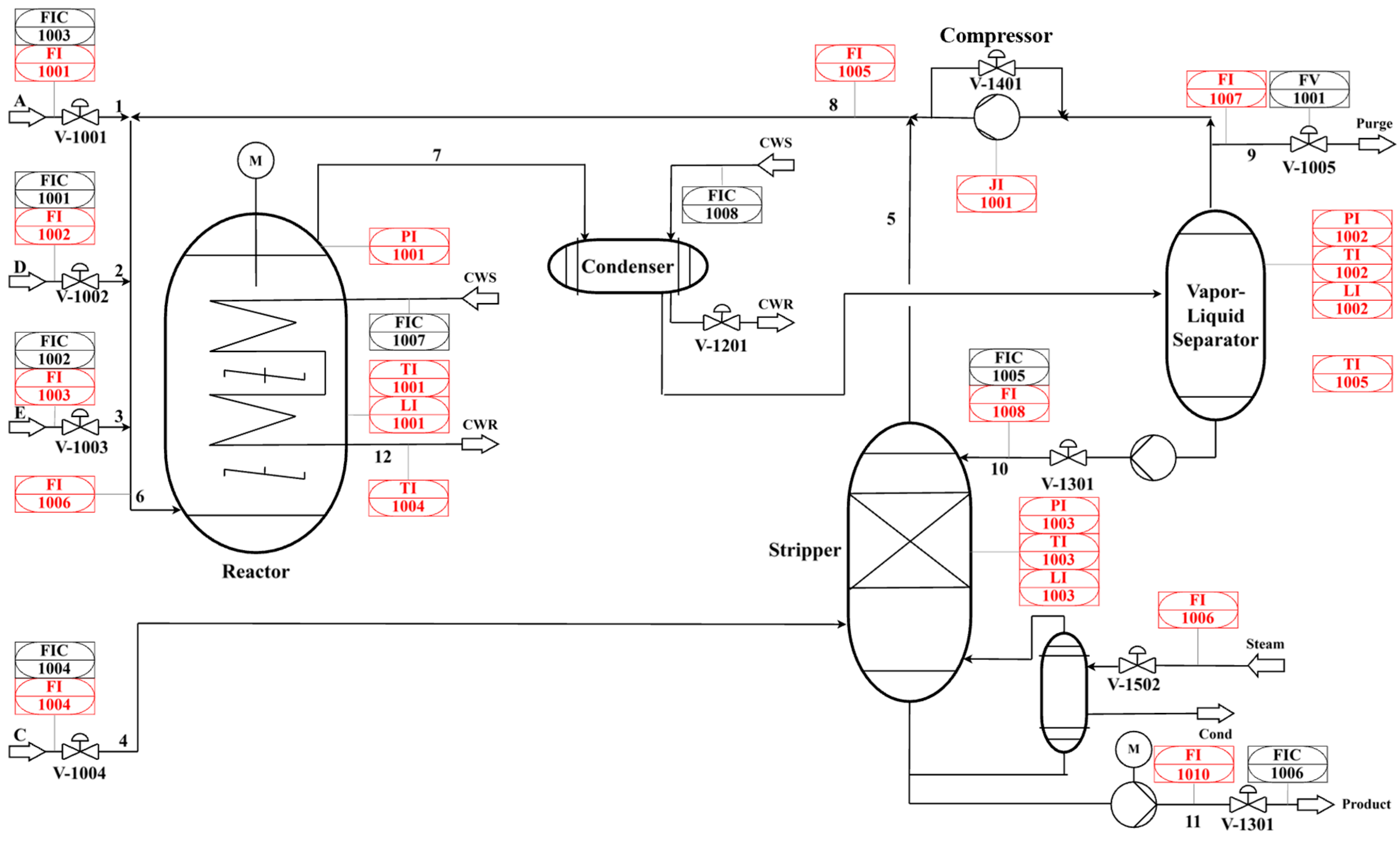To achieve unified decision-making, Support Vector Data Description (SVDD) [20] was then adopted to fuse the monitoring statistics from both subspaces. SVDD provides a powerful one-class classification framework that encloses normal operating data within a hypersphere in feature space, allowing effective discrimination between normal and abnormal conditions. This integration not only enhances sensitivity to both steady-state and dynamic faults but also improves robustness against process non-stationarity. The proposed framework was validated on the benchmark Tennessee Eastman (TE) and two industrial processes. Experimental results demonstrate that the proposed framework significantly outperformed conventional SSA and some deep learning-based monitoring methods, offering superior detection accuracy, lower false alarm rates.

2. Theory and Methods

2.1. Stationary Subspace Analysis

SSA is a blind source separation approach that factorizes the observed signal $x\left(t\right)$ into stationary and non-stationary source based on the Equation (1) as follows:

$$x\left(t\right)=As\left(t\right)=\left[A^s,A^n\right]\left[\begin{array}{c}{s}^s\left(t\right)\\ s^n\left(t\right)\end{array}\right]$$

(1)

where $A$ is an invertible matrix. $s^s\left(t\right)$ and $s^n\left(t\right)$ are stationary and non-stationary sources, respectively. The goal of SSA is to separate the stationary sources and non-stationary sources by estimating a separation matrix ad the following:

$$P=A^{-1}=\left[\begin{array}{c}{P}^s\\ P^n\end{array}\right]$$

(2)

$$\left[\begin{array}{c}{s}^s\left(t\right)\\ s^n\left(t\right)\end{array}\right]=A^{-1}x\left(t\right)=\left[\begin{array}{c}{P}^{s}x\left(t\right)\\ P^{n}x\left(t\right)\end{array}\right]x\left(t\right)$$

(3)

where $P^s$ and $P^n$ are the stationary and non-stationary projection matrices.

The process data were first divided into $N$ consecutive and nonoverlapping epochs, $[X_1,X_2\dots \dots X_N]$. For any projection matrix $P$, it was possible to obtain the mean ${\mu }_{s,i}=P^s{\mu }_i$ and covariance matrix ${\Sigma }_{s,i}=P^s{\Sigma }_i$ of stationary sources in each epoch, thus obtaining the distribution $Norm({\mu }_{s,i},{\Sigma }_{s,i})$.

The distance between the stationary sources and the standard normal distribution was calculated in each epoch, which was measured by the Kullback–Leibler divergence $D_{KL}$. $D_{KL}$ were summed over each epoch to construct an objective function as follows:

$$f(P^s)={\sum }_i^N{D}_{KL}\left[Norm\right({\mu }_{s,i},{\Sigma }_{s,i})\Vert Norm\left(0,I\right)].$$

(4)

Equation (4) corresponds to the following optimization objective:

$$min{\sum }_i^N{D}_{KL}[Norm({\mu }_{s,i},{\Sigma }_{s,i})\Vert Norm(0,I)]$$

(5)

$$s.t.P^s{\left(P^s\right)}^T=I.$$

(6)

The problem is usually solved by the gradient descend method to obtain the optimal stationary projection matrix $P^s$ and stationary sources $P^{s}x\left(t\right)$.

2.2. Stacked Autoencoder

The structure of the autoencoder is divided into two parts, the encoder and the decoder, for input data $[x_1,x_2\dots \dots x_n]$, the encoder maps it to the hidden layer of the following form:

$$h=f_e\left(W_{e}x+b_e\right)$$

(7)

where $h$ is the hidden layer features, $W_e$ is the encoder layer weights, $b_e$ is the bias vector, and $f_e$ is the activation function. The decoder reconstructs the hidden layer features to obtain the reconstructed data $\tilde{x}$ with the loss function as the following:

$$loss={\displaystyle \frac{1}{N}}{\sum }_{i=1}^m{‖x_i-{\tilde{x}}_i‖}_2^2.$$

(8)

Stacked autoencoders, on the other hand, were obtained by stacking and combining multiple autoencoders, where the current hidden layer features were used as inputs to the next layer of encoders.

2.3. Support Vector Data Description

The goal of the support vector data description is to find a hypersphere region of minimum size $(\mathit{a},R)$, thus including all the training objects, and when a sample point falls outside the region, the sample can be considered as an anomaly.

Its optimization problem can be formulated as follows:

$$\min R^2+C{\sum }_{i=1}^N{\xi }_i$$

(9)

$${‖\phi \left({\mathit{z}}_{\mathit{i}}\right)-\mathit{a}‖}^2\le R^2+{\xi }_i,{\xi }_i\ge 0,i=\mathrm{1,2},\dots ,N.$$

(10)

The radius of the hypersphere was calculated through nonlinear mapping by kernel function $K(·,·)$ as the following:

$$R=\sqrt{K\left(x_v,x_v\right)-2{\sum }_{i=1}^n{a}_{i}K\left(x_v,x_i\right)+{\sum }_{i=1}^n{\sum }_{j=1}^n{a}_i{a}_{j}K\left(x_i,x_j\right)}.$$

(11)

The Gaussian kernel function is employed as the following:

$$K\left(x_i,x_j\right)=\mathrm{e}\mathrm{x}\mathrm{p}(-{\displaystyle \frac{{‖x_i-x_j‖}^2}{2{\sigma }^2}}).$$

(12)

For a new sample $z$, the distance $d$ to the center of the hypersphere region can be calculated using the following equation:

$$d=\sqrt{K\left(z,z\right)-2{\sum }_{i=1}^n{a}_{i}K\left(z,x_i\right)+{\sum }_{i=1}^n{\sum }_{j=1}^n{a}_i{a}_{j}K\left(x_i,x_j\right)}.$$

(13)

If $d>R$, it is considered that a fault may have occurred.

2.4. Proposed Monitoring Strategy

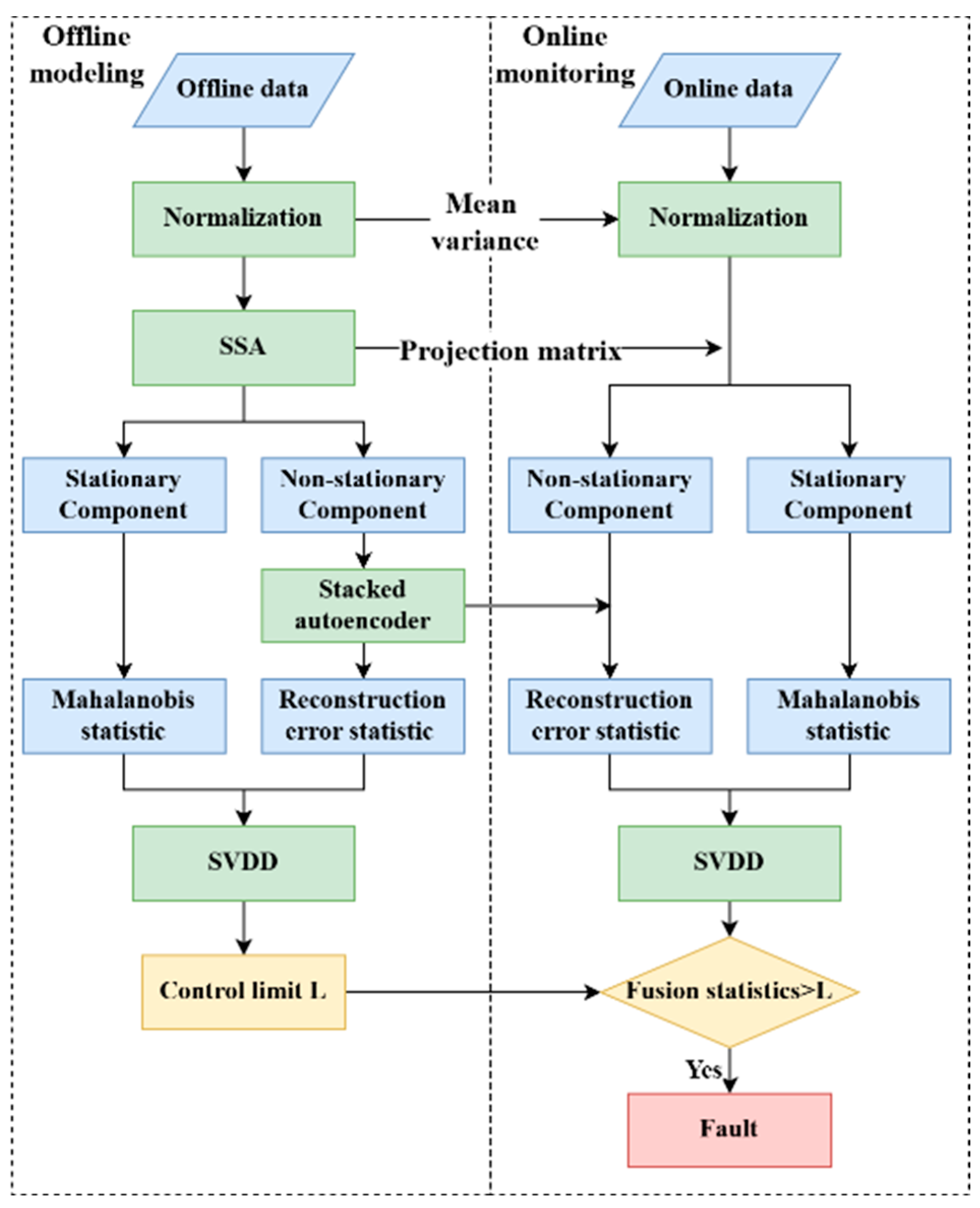
The modeling and implementation steps of the method are shown in Figure 1, which is mainly divided into two parts: offline modeling and online monitoring.

Offline modeling

The offline modeling consists of the following steps:

Step 1: The training data were normalized with Equation (14):

$$X_t=(X_t-\overline{X_t})/s$$

(14)

where $\overline{X_t}$ and $s$ denote the sample mean and the standard deviation of the training data, respectively.

Step 2: SSA was employed on the normalized data to extract the stationary and non-stationary components. A Mahalanobis distance statistic was established for the stationary components, while the non-stationary components were input into a stacked autoencoder.

Step 3: The SAE model was established to reconstruct the non-stationary components, and a monitoring statistic based on reconstruction error is then established.

Step 4: The two statistics were concatenated together, and each statistic can be regarded as a spatial coordinate of a sampling point. Then, all sampling points were mapped to a high-dimensional space via SVDD to find a hypersphere region of minimum size. The radius of the hypersphere is the control limit.

Online monitoring

The online modeling consists of the following steps:

Step 1: The online data were normalized by the mean and variance of the offline data.

Step 2: The normalized data were projected into stationary and non-stationary subspace. A Mahalanobis distance statistic was established for the stationary subspace, while the non-stationary components were input into the trained stacked autoencoder.

Step 3: The non-stationary components were reconstructed by the trained SAE model to obtain the reconstruction error-based statistics.

Step 4: The two statistics were concatenated and mapped by SVDD to obtain the distance between a new sample and the hypersphere’s center, which is the fusion statistics. When the fusion statistics exceed the control limits, it is deemed that a fault has occurred.

3. Results and Discussion

3.1. TE Case

The TE process, developed by Eastman Chemical Company [21,22], is a chemical simulation process consisting of 5 units and 53 variables. The TE process includes 21 pre-define faults, which are usually used to verify the performance of monitoring methods. A total of 19 variables in the TE process are component variables and their sampling frequency is lower than that of other variables and one variable remains constant, which is usually not selected in process monitoring tasks. Thus, we selected the remaining 33 process variables. The process flow chart of the TE process is shown in Figure 2, and the variables information is shown in

Table 1. Variables information of the TE process.

Variables	Details	Variables	Details	Variables	Details
F1	A feed (stream 1)	L12	Product separator level	V23	D feed flow (stream 2)
F2	D feed (stream 2)	P13	Product separator pressure	V24	E feed flow (stream 3)
F3	E feed (stream 3)	F14	Product separator underflow (stream 10)	V25	A feed flow (stream 1)
F4	A and C feed (stream 4)	L15	Stripper level	V26	A and C feed flow (stream 4)
F5	Recycle flow (stream 8)	P16	Stripper pressure	V27	Compressor recycle valve
F6	Reactor feed rate (stream 6)	F17	Stripper underflow (stream 11)	V28	Purge valve (stream 9)
P7	Reactor pressure	T18	Stripper temperature	V29	Separator pot liquid flow (stream 10)
L8	Reactor level	F19	Stripper steam flow	V30	Stripper liquid prod flow (stream 11)
T9	Reactor temperature	C20	Compressor work	V31	Stripper steam valve
F10	Purge rate (stream 9)	T21	Reactor cooling water outlet temperature	V32	Reactor cooling water flow
T11	Product separator temperature	T22	Separator cooling water outlet temperature	V33	Condenser cooling water flow

. The fault details are described in

Table 2. Fault information of the TE process.

No.	Fault Description	Fault Type
1	A/C feed ratio, B composition constant (stream 4)	Step
2	B composition, A/C ratio constant (stream 4)	Step
3	D feed temperature (stream 2)	Step
4	Reactor cooling water inlet temperature	Step
5	Condenser cooling water inlet temperature	Step
6	A feed loss (stream 1)	Step
7	C header pressure loss-reduced availability (stream 4)	Step
8	A, B, C feed composition (stream 4)	Random variation
9	D feed temperature (stream 2)	Random variation
10	C feed temperature (stream 4)	Random variation
11	Reactor cooling water inlet temperature	Random variation
12	Condenser cooling water inlet temperature	Random variation
13	Reaction kinetics	Slow drift
14	Reactor cooling water valve	Sticking
15	Condenser cooling water valve	Sticking
16	Unknown	-
17	Unknown	-
18	Unknown	-
19	Unknown	-
20	Unknown	-
21	The valve for stream 4	Constant position

. For each fault, the same training set was employed which comprising 500 sampling points, and the test set contains 960 sampling points, and each fault is introduced at the 160th sampling point.

The traditional principal component analysis (PCA), SSA, SAE, variational autoencoders (VAE), and nSSA-SAE, which only consider non-stationary spatial reconstruction errors, and an SSA-one class support vector machine (SSA-OCSVM) [23] were compared with proposed integrated monitoring framework. The SAE consists of three encoding and decoding layers. The ReLU activation function was applied in all hidden layers. The model was trained through the Adam optimizer with a learning rate of 0.001 and a mean squared error (MSE) loss function. Fault Detection Rate (FDR), False Alarm Rate (FAR), and Fault Detection Time (FDT) (the index corresponding to five consecutive alarm sample points) were applied to evaluate the process monitoring performance, which can be calculated by following Equations (15) and (16). The results are shown in

Table 3. Comparison monitoring results (FDR)% of 21 faults in the TE process.

Fault No.	PCA (T2)	PCA (Q)	SSA	SSA-OCSVM	VAE	SAE	nSSA-SAE	Proposed
1	99.2	100.0	99.6	99.6	100.0	99.9	99.9	99.9
2	98.2	99.0	98.2	98.4	98.9	98.9	99.1	98.9
3	/	/	/	/	/	/	/	/
4	31.1	100.0	98.8	100.0	100.0	99.9	100.0	100.0
5	27.8	26.9	100.0	100.0	40.0	35.0	100.0	100.0
6	99.4	100.0	100.0	100.0	100.0	100.0	100.0	100.0
7	100.0	100.0	99.8	100.0	100.0	100.0	100.0	100.0
8	97.4	94.9	98.1	97.0	98.9	98.9	98.4	98.2
9	/	/	/	/	/	/	/	/
10	45.6	49.6	88.6	81.2	66.6	58.2	90.0	91.1
11	48.1	80.5	72.9	78.6	83.8	78.6	77.9	80.8
12	98.5	94.6	99.9	99.5	99.8	99.4	99.9	99.9
13	94.2	95.2	95.5	95.6	95.5	95.4	95.4	95.4
14	99.5	100.0	100.0	100.0	100.0	100.0	99.9	100.0
15	/	/	/	/	/	/	/	/
16	30.0	47.6	89.5	87.8	65.4	41.5	88.6	93.8
17	80.0	96.0	93.9	96.2	96.5	94.9	95.8	96.8
18	89.9	90.5	90.5	91.0	91.2	90.4	90.4	90.1
19	14.5	28.9	81.9	88.4	54.8	25.6	86.5	93.6
20	42.5	60.0	88.5	87.5	69.2	65.4	90.4	91.2
21	40.6	56.1	42.4	43.0	57.9	51.2	64.8	63.4
Average	68.7	78.9	90.1	91.3	84.4	79.6	93.2	94.1

,

Table 4. Comparison monitoring results (FAR)% of 21 faults in the TE process.

Fault No.	PCA (T2)	PCA (Q)	SSA	SSA-OCSVM	VAE	SAE	nSSA-SAE	Proposed
1	0.0	1.9	1.2	8.1	5.0	5.6	0.0	1.2
2	1.2	2.5	0.0	5.6	3.1	5.0	0.0	3.8
3	/	/	/	/	/	/	/	/
4	1.2	3.1	3.1	5.0	5.6	6.2	1.2	0.6
5	1.2	3.1	3.1	5.0	5.6	6.2	1.2	0.6
6	0.6	1.2	1.9	4.4	4.4	2.5	0.0	1.2
7	1.2	2.5	2.5	4.4	8.1	3.8	0.0	0.6
8	0.6	1.2	1.9	5.0	4.4	6.2	1.9	1.9
9	/	/	/	/	/	/	/	/
10	1.2	1.9	1.2	3.8	7.5	7.5	0.6	1.9
11	1.2	4.4	3.1	3.8	10.6	10.0	2.5	2.5
12	1.2	2.5	2.5	5.0	6.9	6.9	0.6	2.5
13	0.0	0.6	0.6	3.1	3.8	5.0	0.6	1.2
14	0.6	3.1	2.5	3.1	6.9	8.8	0.6	1.2
15	/	/	/	/	/	/	/	/
16	11.9	5.0	6.9	6.2	17.5	24.4	16.2	11.9
17	1.2	3.9	1.9	8.1	10.0	7.5	1.9	1.9
18	0.6	2.5	0.6	5.0	10.6	4.4	1.2	1.2
19	0.0	1.2	1.9	5.0	6.2	3.8	0.0	0.0
20	0.6	1.9	0.6	8.1	3.8	3.1	0.0	1.2
21	1.9	6.9	5.6	8.1	10.6	9.4	6.9	5.0
Average	1.5	2.7	2.3	5.4	7.3	7.0	2.0	2.3

and

Table 5. Comparison monitoring results (FDT) of 21 faults in the TE process.

Fault No.	PCA (T2)	PCA (Q)	SSA	SSA-OCSVM	VAE	SAE	nSSA-SAE	Proposed
1	167	161	165	167	161	163	162	161
2	175	171	176	178	172	172	171	171
3	/	/	/	/	/	/	/	/
4	317	161	163	161	161	161	161	161
5	161	163	161	161	161	161	161	161
6	167	161	161	161	161	161	161	161
7	161	161	161	161	161	161	161	161
8	186	180	180	183	169	174	178	178
9	/	/	/	/	/	/	/	/
10	226	208	182	185	207	193	182	182
11	171	166	169	165	166	166	166	166
12	182	169	162	163	263	163	162	162
13	207	201	201	203	201	202	198	201
14	161	161	161	161	161	161	162	161
15	/	/	/	/	/	/	/	/
16	196	176	169	167	176	196	170	167
17	189	182	180	179	181	182	180	182
18	248	243	243	239	241	245	244	243
19	961	649	170	171	193	302	162	170
20	244	245	227	229	245	239	227	232
21	625	416	639	656	426	426	415	415
Average	263.6	220.8	203.9	205.0	194.8	201.6	190.2	190.3

and Figure 3.

$$FDR={\displaystyle \frac{Numberofcorrectalarmsamples}{Faultsamples}}$$

(15)

$$FAR={\displaystyle \frac{Numberoffalsealarmsamples}{Normalsamples}}$$

(16)

It has been demonstrated in many existing studies that faults 3, 9, and 15 are difficult to monitor due to their tiny deviation and are therefore not considered in the comparison results. It can be observed in Table 2 and Table 3, the proposed method performed optimally in most faults, especially in faults 5, 10, 16, and 19. This may be due to the introduction of SSA, which can separate stationary and non-stationary components from the original data, making it more sensitive to these faults. It can also be proven by the fact that SSA-based methods, SSA, nSSA-SAE, SSA-OCSVM, and the proposed method, can greatly improve the FDR compared to traditional PCA, VAE, and SAE, which demonstrated the claim that the fault information could be hidden in the non-stationary subspace. In addition, although the FAR of the proposed method is not the lowest, it is within an acceptable range, proving the effectiveness of the proposed method.

Faults 1 and 19 were selected as examples for further analysis. For fault 1, as shown in Figure 4, all methods proved effective in detecting the fault and promptly issuing an alarm upon its occurrence. This is attributable to the relatively straightforward nature of fault 1, where the deviation in variables is substantial when the fault occurs. For fault 19, as shown in Figure 5, however, methods such as PCA, VAE, and SAE, which do not account for process non-stationarity, performed poorly. This may stem from the fault association with non-stationary variables, whereas these methods operate under the assumption of process stationarity. SSA, SSA-OCSVM, and nSSA-SAE, which considered only one aspect of process information (either stationary or non-stationary), consequently exhibited lower fault detection rates. The higher detection rate of nSSA-SAE compared to SSA further underscores the necessity of incorporating non-stationary subspace information. The proposed method in this paper enables timely alarm generation upon fault occurrence and achieves the highest fault detection rate for fault 19, demonstrating its superiority over other SSA-based and reconstruction-based monitoring methods.

3.2. Industrial Case 1

Figure 6 demonstrates the flowchart of a catalytic reforming process of a petrochemical company, which contains four reactors, four heating furnaces and a key equipment, plate heat exchanger. In this process, the feed rates of naphtha and circulating hydrogen are the key factors affecting the pressure drop at the hot end of the plate heat exchanger. Due to external disturbances such as production load adjustment, process variables such as heat exchanger hot end pressure drop and circulating hydrogen feed rate often show obvious non-stationary trends. In actual operation, the hot end pressure drop of the heat exchanger frequently shows an abnormal increase, which brings much trouble to the operator and makes it difficult to accurately determine whether the change is caused by normal fluctuations or potential faults.

In addition, the heat exchange efficiency is influenced by the increase of pressure drop, resulting in increasing fuel gas consumption of the heating furnace. When the pressure drop increases to an unacceptable level, the plant must shut down, which causes a huge loss to upstream and downstream production plans and factory profits. Therefore, effective monitoring of this non-stationary process is of great significance in early abnormal warning, assisting operators to take timely intervention measures, avoiding the expansion of faults, and bringing significant economic benefits to the enterprise.

Figure 7 demonstrates the variation in hot-end pressure drop with hydrogen feed rate and total naphtha feed rate. Due to frequent adjustments in production load, the naphtha feed rate exhibits significant fluctuations, resulting in multiple operating conditions, a characteristic feature of non-steady-state processes. Under normal operating conditions, the hot-end pressure drop typically varies synchronously with both hydrogen and naphtha feed rates, indicating a stable process relationship. However, within the red shaded region, when the naphtha feed rate remains relatively stable, a reduction in the hydrogen feed rate paradoxically causes the hot-end pressure drop to increase, suggesting a potential process malfunction. Thus, 4000 sampling points were selected that included abnormal increases of hot end pressure drop. The sampling frequency was 1 min, and each sampling point consisted of 27 variables, including circulating hydrogen pressure, reactor inlet and outlet pressure difference, and reactor outlet temperature. The detailed information is in

Table 6. Variables information in continuous catalytic reforming process.

No.	Variables Description	No.	Variables Description
1	Inlet flow of cold end	15	Inlet temperature of hot end
2	Hydrogen flow rate	16	Inlet temperature of cold end
3	Inlet pressure of cold end	17	Outlet temperature of cold end
4	Hydrogen pressure	18	Outlet temperature of the first furnace
5	Outlet pressure of hot end	19	Outlet temperature of the second furnace
6	Pressure drops of hot end	20	Outlet temperature of the first reactor
7	Pressure drops of cold end	21	Outlet temperature of the second reactor
8	Pressure drops of the first reactor	22	Outlet temperature of the third furnace
9	Pressure drops of the second reactor	23	Outlet temperature of the third reactor
10	Pressure drops of the third reactor	24	Outlet temperature of the fourth furnace
11	Pressure drops of the fourth reactor	25	Temperature drops of the third furnace
12	Inlet pressure of the fourth reactor	26	Temperature drops of the fourth furnace
13	Pressure drops of cold end filter	27	Temperature drops of the second furnace
14	Outlet temperature of hot end

. The first 2500 sampling points were used as offline data to train the monitoring model, while the remaining 1500 sampling points were used as online data to validate the performance of the monitoring model. Around the 460th point in the test set, an abnormal increase in hot end pressure drop occurred.

The monitoring results of compared methods mentioned before are shown in Figure 8 and

Table 7. Comparison monitoring results of industrial process 1.

Methods	FDR (%)	FAR (%)	FDT
PCA (T2)	5.96	2.61	/
PCA (Q)	100.00	24.78	300
SSA	99.42	39.13	270
SSA-OCSVM	93.17	30.87	321
VAE	100.00	54.57	130
SAE	87.31	13.70	384
nSSA-SAE	99.62	8.04	450
Proposed	99.04	4.78	465

.

As shown in Figure 8, the PCA (T2) failed to detect the fault and although PCA (Q), SSA-based, VAE, and SAE-based methods can detect faults, they also generated many false alarms even there was no fault occurs, which may mislead operators and lead to incorrect operations. The nSSA-SAE method effectively reduced the probability of the model identifying normal non-stationary trends as faults by considering fault information in non-stationary subspaces. However, its false alarm rate was still higher than that of the method proposed. Although the FDR of proposed integrated monitoring framework was slightly lower than nSSA-SAE, it significantly reduced the FAR compared to the comparison methods, demonstrating the rationality of jointly considering stationary and non-stationary information and proving the effectiveness of the proposed method. Although the FDT of some methods was lower than that of the proposed method, this is attributable to false alarms and is therefore unreliable. Consequently, the FDT serves as a less significant measure of model performance in this case.

We further analyzed the impact of the number of stationary component and depth of SAE on the performance of proposed method, taking this case as an example.

Figure 9 demonstrates that the number of stationary components has little effect on the FDR, with all FDR values achieving a high level. The FAR is minimized (lower than 5%) when the number of stationary components equals six (selected in this work), which indicates that the fault information is more concealed within the non-stationary components, and the detection of this fault is primarily contributed by reconstruction error.

In Figure 10, the FDR for most models reached 95%, with a FAR below 5%. However, due to the inherent uncertainty in deep learning model training, it remains unclear how the number of SAE layers affects FDR and FAR in this case. Nevertheless, it is certain that higher layer counts necessitate greater computational resources for both training and inference. Consequently, the number of SAE layers should not be excessively high.

3.3. Industrial Case 2

An industrial Dimethyl Ether/Methanol to Olefin (DMTO) of a chemical company in China was investigated as the second industrial case study to demonstrate the performance of the proposed framework in industrial non-stationary processes monitoring. The DMTO process is an advanced coal-to-chemicals technology that converts methanol or dimethyl ether into light olefins, mainly ethylene and propylene, through catalytic reactions. In industrial applications, the DMTO process exhibited highly complex dynamics due to catalyst deactivation, strong nonlinear coupling among temperature, pressure, and flowrate variables in the process. The detailed information is in

Table 8. Variables information in DMTO.

Variables Tag	Variable	Variables Tag	Variable
TI1101D	Reactor 1 Dense phase temperature	PIC1405	Methanol-steam/stripping gas heat exchanger outlet methanol gas pressure
TI1101E	Reactor 1 Dense phase temperature	PIC1604	Scrubbing tower top pressure
TI1110	Reactor 1 Top outlet gas temperature	PDI1102	Reactor 1 Cyclone Separator Pressure difference
TI1111A	Reactor 1 Cyclone separator inlet temperature	PDI1104A	Reactor 1 Distributor Total Differential Pressure
TI1111B	Reactor 1 cyclone separator inlet temperature	PDI1104B	Reactor 1 Distributor Total Differential Pressure
TI1111C	Reactor 1 cyclone separator inlet temperature	TI1412	Heat exchanger 2A/B Outlet Stripper Gas Temperature
TI1111D	Reactor 1 cyclone separator inlet temperature	TI1413A	Heat exchanger 1A outlet methanol temperature
TI1112A	Reactor 1 Dilute phase bed bottom temperature	TI1413B	Heat exchanger 1A outlet methanol temperature
TI1112B	Reactor 1 Dilute phase bed bottom temperature	TI1413C	Heat exchanger 2A outlet methanol temperature
TI1112C	Reactor 1 Dilute phase bed bottom temperature	TI1413D	Heat exchanger 2A outlet methanol temperature
TI1112D	Reactor 1 Dilute phase bed bottom temperature	TI1414	Methanol-steam/stripper gas heat exchanger outlet methanol temperature
TI1113A	Reactor 1 Dense phase bed top temperature	FIC1403	Methanol feed rate
TI1113B	Reactor 1 Dense phase bed top temperature	TI1134B	Reactor 2 Dense phase bed bottom temperature
TI1113C	Reactor 1 Dense phase bed top temperature	TI1134C	Reactor 2 Dense phase bed bottom temperature
TI1113D	Reactor 1 Dense phase bed top temperature	TI1134D	Reactor 2 Dense phase bed bottom temperature
TI1115	Reactor 1 Dense phase bed bottom temperature	TI1134E	Reactor 2 Dense phase bed bottom temperature
TI1116A	Reactor 1 Upper Stripping Temperature	TI1135A	Reactor 2 Upper Stripping Temperature
TI1116B	Reactor 1 Lower Stripping Temperature	TI1130A	Reactor 2 Cyclone separator inlet temperature
TI1122A	Reactor 1 Transition Temperature	TI1131A	Reactor 2 Dilute phase temperature
TI1122B	Reactor 1 Transition Temperature	TI1131B	Reactor 2 Dilute phase temperature
TI1122C	Reactor 1 Transition Temperature	TI1131C	Reactor 2 Dilute phase temperature
TI1122D	Reactor 1 Transition Temperature	TI1131D	Reactor 2 Dilute phase temperature

.

A section of historical production data collected by DCS with a total of 7500 samples was selected for validate the monitoring performance of proposed and compared methods. The sampling interval was 15 s and each sample contained 44 process variables, including temperature, pressure, flow rate, and variables associated with devices such as the two main reactors in DMTO.

Figure 11 illustrates the four variables for measuring the main reactor dense phase bed bottom temperature. At about the 1070th point (the red line), an unknown offset occurred in 1190TI1134E, whereas before that, these variables retained a similar change trend, which suggests that a fault has occurred.

Figure 12 illustrates the performance of the proposed method and comparative approaches in monitoring the DMTO process. As shown, PCA T2 and SAE exhibited delayed alarm times and failed to sustain alarms after faults occurred due to their insensitivity to non-stationary processes. Due to the assumption of a normal distribution in its latent space, the VAE may not be applicable for resampling non-stationary variables, thereby rendering it alarms almost the whole test set. Meanwhile, PCA-SPE and nSSA-SAE, which reconstructs solely for non-stationary components, generated a small number of false alarms before faults occurred, resulting in higher false alarm rates, and SSA-OCSVM also exhibited a similar situation. SSA and the proposed method exhibited similar performance, but SSA also showed a relatively high false alarm rate, which may lead to misjudgment by operators. As shown in

Table 9. Comparison monitoring results of industrial process 2.

Methods	FDR (%)	FAR (%)	FDT
PCA (T2)	64.87	1.78	/
PCA (Q)	99.29	32.71	/
SSA	97.79	4.49	1091
SSA-OCSVM	99.38	17.57	/
VAE	100.00	91.12	/
SAE	81.77	7.01	/
nSSA-SAE	100.00	9.35	960
Proposed	99.47	1.31	1071

, although the FDR of proposed method was not the highest, it still achieved 99.47%, which meets industrial practice requirements. Furthermore, its FAR reached 1.31%. Overall, the proposed method demonstrated the best performance in the DMTO process.

4. Conclusions

This work tackles the challenge of non-stationary processes monitoring by proposing a novel joint monitoring framework that integrates stationary subspace analysis (SSA) with stacked autoencoders (SAE). The proposed method effectively captures both stationary and non-stationary features, enabling the identification of latent fault information and improving fault detection performance under non-stationary conditions. In practical production scenarios, it can successfully differentiate between normal process variations and abnormal behaviors, providing timely fault warnings and significantly reducing the false alarm probability. And it can detect minor abnormalities in the process to avoid accidents, resulting in economic losses or even casualties. Experimental results demonstrate that the proposed approach outperforms conventional process monitoring methods in terms of detection accuracy and robustness.

In fact, this method can adapt to different processes by adjusting the weight coefficients of the stationary subspace monitoring statistics and the non-stationary reconstruction error statistics. To consider the dynamic system, the process time lag can be introduced. We will study this part in the future.