Fast Calculation Method of Two-Phase Flow in Horizontal Gas Wells Based on PI-DeepONet

Abstract

With the deepening of unconventional oil and gas resource development, the gas–liquid two-phase flow phenomenon in horizontal gas wells is becoming increasingly complex. Accurate and efficient prediction of the flow state has become key to optimizing production. While traditional numerical simulation methods are highly accurate, their long calculation times make them unsuitable for real-time applications. Conversely, purely data-driven methods struggle with accuracy under sparse data conditions. This paper proposes a deep operator network method (PI-DeepONet) that integrates physical prior knowledge—specifically the drift-flux model—to rapidly predict two-phase flow parameters. By jointly training the network with both data loss and physical loss, the model’s accuracy and generalization are significantly enhanced. Comparing the results with the OLGA numerical simulator verifies the model’s high performance. The average relative error of the PI-DeepONet on the test set is less than 1%, with the error of some physical quantities controlled within 0.2%. Critically, the single prediction time is less than 0.1 s, achieving a calculation speed nearly 50,000 times higher than the traditional numerical simulation method. The model significantly improves prediction speed while ensuring accuracy, making it ideal for real-time simulation and rapid response requirements in horizontal wells. This study provides a new path for intelligent diagnosis and prediction of underground working conditions and demonstrates broad engineering application potential.

1. Introduction

With the rapid development of the global economy, the demand for energy in various countries is increasing year by year [1]. In recent years, shale gas has become the main resource for increasing reserves and production in China’s natural gas sector, and occupies an important position in oil and gas energy extraction [2]. Horizontal wells can increase the gas leakage area and improve the utilization rate of gas reservoirs, and have gradually become the main means of developing shale gas and tight gas [3]. However, a large amount of fracturing fluid backflow and water production in the reservoir itself caused water to appear at the beginning of gas well production, and gas–liquid two-phase flow occurred in the wellbore [4]. Correctly predicting the gas–liquid two-phase flow pattern in horizontal gas wells is a prerequisite for predicting the wellbore pressure drop, diagnosing downhole conditions, and designing drainage and gas production [5,6,7]. Traditional numerical methods such as finite difference method, finite element method, and finite volume method are often used to analyze the two-phase flow in horizontal gas wells [8,9,10]. Although these methods are highly accurate, they are computationally intensive and time-consuming [11]. The classic deep learning method is mainly driven by pure data. It repeatedly trains and learns from a given neural network structure and the obtained training data to obtain a specific model, that is, to establish a mapping relationship from input data to output data that conforms to the laws of the physical model as much as possible. This method relies on the high accuracy of given data and massive amounts of training data, but ignores the prior knowledge contained in these data in actual physical scenarios (such as physical laws such as conservation of mass and momentum), resulting in a waste of information resources [12].

In recent years, deep learning has been gradually applied to the field of scientific computing, providing new solutions to address the above challenges [13]. This trend’s transformative potential is evident across diverse scientific domains, with successful applications ranging from the clinical diagnosis of gastric cancer from histopathological images to the automated, vision-based analysis of transport properties in cementitious materials [14,15]. Among them, the Physics-informed Neural Network (PINN) [16] has shown significant advantages in solving partial differential equations. PINN embeds physical prior knowledge into neural networks and can be trained in a semi-supervised learning manner. Although PINN has achieved certain results in solving PDEs, it still cannot effectively handle parameterized partial differential equations because retraining is required when changing parameters, which increases the time cost. To this end, Lu et al. [17] proposed a new solution method based on the concept of operator learning, namely the Deep Operator Network (DeepONet). Deep operator neural networks learn linear or nonlinear operators based on data and have the advantages of fast convergence speed and strong generalization ability. Currently, DeepONet has been used to solve heat conduction equations [18], fluid equations [19], etc. However, due to the lack of physical prior knowledge, DeepONet is essentially a pure data-driven method, and the accuracy of model training depends entirely on the amount of data. In the actual horizontal gas well two-phase flow problem, the downhole detection points and data points are relatively sparse, and the prediction accuracy of the pure data neural network model is difficult to guarantee, which needs to be improved.

To address the shortcomings of pure data-driven neural network methods, Wang et al. [20] introduced physical equations into DeepONet training and proposed a physical information deep operator network (PI-DeepONet) method. Since this method introduces the constraints of physical equations during the training process, the solution accuracy is greatly improved compared to the pure data-driven DeepONet method, and the amount of training data required is relatively small.

Based on the above background, this paper proposes for the first time a fast calculation method for two-phase flow in horizontal gas wells based on PI-DeepONet. The main innovations of this study are: (1) integrating the drift flux model as a physical constraint into the deep operator network, significantly improving the model’s prediction accuracy and generalization ability with small sample data; (2) implementing an end-to-end surrogate model, whose computational speed is increased by four orders of magnitude compared with traditional numerical simulation software (such as OLGA), while maintaining a small mean relative error, thus enabling real-time diagnosis and optimization of downhole conditions. The structure of this paper is as follows: In Section 1, the theoretical model of gas–liquid two-phase flow, namely the drift flux model, is introduced. Section 2 introduces the basic principles of PI-DeepONet and the calculation process of the drift flux model based on PI-DeepONet. Section 3 introduces the actual application and the corresponding results. The conclusion is placed in Section 4.

2. Gas–Liquid Two-Phase Flow Model for Horizontal Gas Wells

The drift-flux model is commonly used in hydraulic models based on transient two-phase flow in wellbore. The drift-flux model has been widely used to describe the phenomenon of gas–liquid two-phase flow in wellbore. The most basic drift-flux model was originally proposed by Zuber and Findlay [21], and later modified by Wallis [22], Ishii [23] and Shi et al. [24]. In order to derive the control equations, the following assumptions are usually made: the gas phase and liquid phase have the same pressure and temperature in the same section; the influence of temperature changes in the wellbore on the gas–liquid parameters is ignored; and the mass transfer between the gas and liquid phases is ignored.

Based on the above assumptions, the control equation system of the drift flow model consists of three equations, namely the gas mass conservation equation, the liquid mass conservation equation and the gas–liquid mixed momentum conservation equation, which are usually described as:

$${\displaystyle \frac{𝜕}{𝜕t}}\left({{\alpha }_g\rho }_g\right)+{\displaystyle \frac{𝜕}{𝜕z}}\left({{\alpha }_g\rho }_g{v}_g\right)=0$$

(1)

$${\displaystyle \frac{𝜕}{\mathsf{\partial }t}}\left({{\alpha }_l\rho }_l\right)+{\displaystyle \frac{𝜕}{𝜕z}}\left({{\alpha }_l\rho }_l{v}_l\right)=0$$

(2)

$${\displaystyle \frac{𝜕}{𝜕t}}\left({{\alpha }_g\rho }_g{v}_g+{\alpha }_l{\rho }_l{v}_l\right)+{\displaystyle \frac{𝜕}{𝜕z}}\left({{\alpha }_g\rho }_g{v}_g^2+{\alpha }_l{\rho }_l{v}_l^2+p\right)=F_w+{\rho }_{m}gsin\theta$$

(3)

Among them, ${\alpha }_g$ and ${\alpha }_l$ are the gas holdup and liquid holdup, respectively; ${\rho }_g$ and ${\rho }_l$ are the gas density and liquid density, respectively; ${\rho }_m$ is the gas–liquid mixture density, with the unit of $\mathrm{k}\mathrm{g}/{\mathrm{m}}^3$; $v_g$ and $v_l$ are the absolute phase velocities of the gas and liquid, respectively, with the unit of m/s; $p$ is the pressure of the two phases, with the unit of $\mathrm{P}\mathrm{a}$; $\theta$ is the inclination angle (the angle between the wellbore and the horizontal direction); $F_w$ is the wall friction force per unit length, with the unit of $\mathrm{N}/\mathrm{m}$; and $t$ and $z$ represent time and axial position, with the units of $\mathrm{s}$ and $\mathrm{m}$, respectively.

The calculation area of the drift flux model is shown in Figure 1.

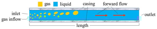
Figure 1. Schematic diagram of the calculation area of the drift flux model.

Because there are seven unknown variables (${\alpha }_g$, ${\alpha }_l$, ${\rho }_g$, ${\rho }_l$, $v_g$, $v_l$, $p$) and three governing equations, additional closed-form equations are required to complete the solution of the governing equations. Assume that the liquid density has the following form:

$${\rho }_l={\rho }_{l,0}+{\displaystyle \frac{p-p_{l,0}}{a_l^2}}$$

(4)

where $a_l$ is the liquid phase sound velocity, with the unit of $\mathrm{m}/\mathrm{s}$; and ${\rho }_{l,0}$, $p_{l,0}$ are the liquid density and pressure under reference conditions. The gas density is described by the gas law:

$${\rho }_g={\displaystyle \frac{pM}{z_{g}RT}}$$

(5)

where $M$ is the molecular weight of the gas, with the unit of $\mathrm{k}\mathrm{g}/\mathrm{m}\mathrm{o}\mathrm{l}$; $z_g$ is the gas compressibility factor, a dimensionless constant; $R$ is the gas constant; and $T$ is the temperature. To enforce the volume conservation principle, the volume fractions of the gas and liquid phases are related as follows:

$${\alpha }_g+{\alpha }_l=1$$

(6)

Since there is only one gas–liquid mixture momentum equation in the drift flow model, a constitutive equation is required to describe the relative motion between the gas and liquid phases. The slip law of one of the closed equations is given by:

$$v_g={C_{0}v}_m+v_d$$

(7)

where $C_0$ is the distribution coefficient and $v_d$ is the drift velocity. This paper adopts the drift flow model of Bhagwat and Ghajar [25], which is a flow pattern-independent correlation applicable to wellbores with inclinations of −90° to 90°. In this model, the distribution coefficient $C_0$ is expressed as:

$$C_0={\displaystyle \frac{2-{(\frac{{\rho }_g}{{\rho }_l})}^2}{1+{(\frac{{Re}_{tp}}{1000})}^2}}+{\displaystyle \frac{[(\sqrt{\frac{(1+{(\frac{{\rho }_g}{{\rho }_l})}^2\mathrm{c}\mathrm{o}\mathrm{s}\theta )}{(1+\mathrm{c}\mathrm{o}\mathrm{s}\theta )}}){(1-{\alpha }_g)}^{\frac{2}{5}}]+C_{\mathrm{0,1}}}{1+{(\frac{1000}{{Re}_{tp}})}^2}}$$

(8)

The expression of $C_{\mathrm{0,1}}$ is as follows:

$$C_{\mathrm{0,1}}=\left\{\begin{array}{c}0, -{50}^{\circ }\le \theta \le 0^{\circ }andF{r}_{sg}\le 0.1\\ (C_1-C_1\sqrt{{\displaystyle \frac{{\rho }_g}{{\rho }_l}}})[(2.6-\beta {)}^{0.15}-\sqrt{f_{tp}}](1-x{)}^{1.5},otherwise\end{array}\right.$$

(9)

Among them, $C_1$ is a constant of 0.2, $\beta$ represents the gas volume flow fraction, $x$ represents the gas mass flow fraction, $F{r}_{sg}$ is the Froude number, $f_{tp}$ is the Fanning friction factor, ${Re}_{tp}$ is the gas–liquid phase flow Reynolds number, and their expressions are as follows:

$$\beta ={\displaystyle \frac{{{\alpha }_{g}v}_g}{{{\alpha }_{g}v}_g+{{\alpha }_{l}v}_l}}$$

(10)

$$x={\displaystyle \frac{{\dot{m}}_g}{{\dot{m}}_g+{\dot{m}}_l}}={\displaystyle \frac{{{\alpha }_g{\rho }_{g}v}_g}{{{\alpha }_g{\rho }_{g}v}_g+{{\alpha }_l{\rho }_{l}v}_l}}$$

(11)

$$F{r}_{sg}=\sqrt{{\displaystyle \frac{{\rho }_g}{{\rho }_l-{\rho }_g}}}{\displaystyle \frac{{{\alpha }_{g}v}_g}{\sqrt{g{D}_{h}cos\theta }}}$$

(12)

$$f_{tp}=0.0925{R{e}_{tp}}^{-0.2534}+{\displaystyle \frac{13.98{R{e}_{tp}}^{-0.9501}-0.0925{R{e}_{tp}}^{-0.2534}}{{(1+{(\frac{R{e}_{tp}}{293})}^{4.864})}^{0.1972}}}$$

(13)

$${Re}_{tp}={\displaystyle \frac{v_m{\rho }_m{D}_h}{{\mu }_m}}$$

(14)

In the above expressions, ${\dot{m}}_g$, ${\dot{m}}_l$ represent the mass flow rates of gas and liquid, respectively, $D_h$ is the wellbore diameter, and ${\mu }_m$ is the dynamic viscosity of the gas–liquid mixture. The drift velocity $v_d$ is expressed as:

$$v_d=(0.35sin \theta +0.45cos \theta )\times \sqrt{{\displaystyle \frac{g{D}_h\left({\rho }_l-{\rho }_g\right)}{{\rho }_l}}}(1-{\alpha }_g{)}^{0.5}{C}_2{C}_3{C}_4$$

(15)

$C_2$, $C_3$ and $C_4$ are variables that consider the effects of liquid dynamic viscosity, surface tension and wellbore inclination on drift velocity. Their expressions are:

$$C_2=\left\{\begin{array}{c}{[{\displaystyle \frac{0.434}{\mathit{log}(\frac{{\mu }_l}{0.001})}}]}^{0.15},({\displaystyle \frac{{\mu }_l}{0.001}})>10\\ 1,({\displaystyle \frac{{\mu }_l}{0.001}})\le 10\end{array}\right.$$

(16)

$$C_3=\left\{\begin{array}{c}{({\displaystyle \frac{La}{0.025}})}^{0.9},La>0.025\\ 1,La\ge 0\end{array}\right.$$

(17)

$$C_4=\left\{\begin{array}{c}-1,-{50}^{\circ }\le \theta \le 0^{\circ }andF{r}_{sg}\le 0.1\\ 1,otherwise\end{array}\right.$$

(18)

where $La$ is the Laplace variable, expressed as:

$$La={\displaystyle \frac{\sqrt{\frac{\sigma }{g({\rho }_l-{\rho }_g)}}}{D_h}}$$

(19)

where $\sigma$ is the surface tension coefficient of the liquid. The expression of the wall friction force $F_w$ is:

$$F_w={\displaystyle \frac{f{\rho }_m{v}_m^2}{2D_h}}$$

(20)

where $f$ is the friction factor, expressed as follows:

$$f={[-2.34log({\displaystyle \frac{ϵ}{1.72D_h}}-{\displaystyle \frac{9.26}{R{e}_{tp}}}log({({\displaystyle \frac{ϵ}{29.36D_h}})}^{0.95}+{({\displaystyle \frac{18.35}{R{e}_{tp}}})}^{1.108}))]}^{-1/2}$$

(21)

where $ϵ$ is the wall roughness.

3. Fast Solution Method Based on PI-DeepONet

3.1. PI-DeepONet Network Basic Principles

DeepONet is designed based on the universal approximation theorem of operators [26], which was first proposed by Lu et al. As the first operator learning model for solving infinite-dimensional function space mapping, many researchers have demonstrated the learning ability of this model in practice [27,28,29] and theory [30,31,32]. DeepONet is a high-dimensional framework, as shown in Figure 2.

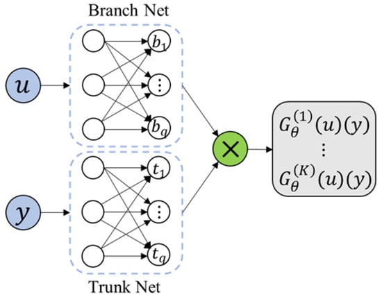
Figure 2. The model of DeepONet.

DeepONet consists of two sub-networks, namely the “trunk” network (Trunk Net) and the “branch” network (Branch Net). The backbone network encodes the spatial and temporal coordinates and outputs a q-dimensional vector $[t_1,t_2,\dots ,t_g{]}^T$. The branch network usually encodes the boundary conditions, initial conditions or source terms of the equation. The input is $\left[u\right(r_1),u(r_2),\dots ,u(r_m){]}^T$, and returns a q-dimensional vector $[b_1,b_2,\dots ,b_g{]}^T$ as output. Finally, the output of DeepONet is obtained by combining the output of the branch network and the backbone network through the inner product. The inner product is expressed as:

$$G_{\theta }\left(u\right)\left(y\right)={\sum }_{k=1}^q{b}_k\left(u\right(r_1),u\left(r_2\right),\dots ,u(r_m))t_k(y)$$

(22)

In the construction of the loss function, DeepONet uses a pure data loss function, which represents the mean square error of the deviation between the predicted value and the true value:

$$L_{data}(\theta )={\displaystyle \frac{1}{pm}}\sum _{j=1}^p\sum _{i=1}^m\left(G_{\theta }\right(u_j\left){(y}_i\right)-G\left(u_j\right){(y}_i){)}^2$$

(23)

Among them, $u_j$ represents the function of different input branch networks, $y_i$ represents the coordinates of the i-th query point, $G_{\theta }\left(u_j\right){(y}_i)$ represents the predicted value of the model, and $G\left(u_j\right){(y}_i)$ represents the corresponding true value.

As can be seen from the above, DeepONet is essentially a pure data-driven neural network method that obtains the best network parameters by fitting the measured values. Therefore, it is also highly dependent on the amount of data. However, in actual engineering problems, data acquisition is more difficult, and pure data-driven methods cannot satisfy the underlying physical laws. To solve such problems, WANG et al. [18] proposed the PI-DeepONet algorithm. The core of this algorithm is to incorporate the physical information part into the loss function, so that the neural network adds the constraints of physical laws. The loss function after adding constraints is expressed as:

$$L\left(\theta \right)={\omega }_d{L}_{data}\left(\theta \right)+{\omega }_p{L}_{physics}\left(\theta \right)$$

(24)

Among them, ${\omega }_d$_d and ${\omega }_p$ represent the weights of the data loss part and the physical loss part respectively.

3.2. Drift-Flux Model Based on PI-DeepONet

This paper proposes a fast calculation method for two-phase flow in horizontal gas wells based on PI-DeepONet. First, the two-phase flow problem in horizontal gas wells is calculated by the finite difference method, and then the calculation results are exported to construct a data set. After that, the boundary condition parameters are sent to the branch network, and the coordinates are sent to the trunk network. The operator is learned through the PI-DeepONet framework, and the first-order derivative is solved by automatic differentiation and passed into the loss function. The loss function consists of data loss and physical loss. The physical loss uses a drift flow model. After the training is completed, PI-DeepONet can perform fast calculations by giving the relevant boundary condition parameters and the coordinates to be solved. The specific process is shown in Figure 3.

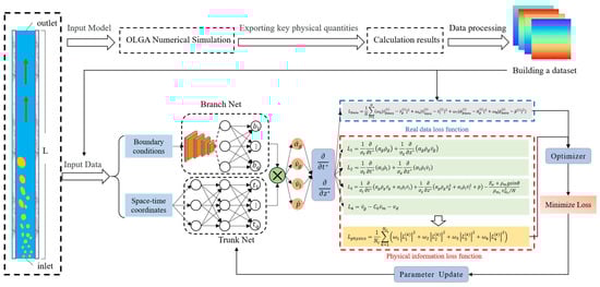
Figure 3. Fast calculation process of two-phase flow in horizontal gas well based on PI-DeepONet.

4. Case Analysis

The training and testing data in this study are all generated from the numerical simulation results of OLGA. The aim is to validate the effectiveness of the proposed method as a surrogate for high-fidelity numerical simulators. This paper takes the horizontal gas well two-phase flow model in Section 1 as an example. First, the oil and gas simulation software OLGA (2022.1.0) is used for modeling and numerical calculation. The calculated data is normalized and then divided into training set/test set. The network is then trained with the training set, and the test set is used to compare the results of the finite difference method and the deep operator model.

4.1. Building a Dataset

As a data-driven model, a certain amount of labeled data needs to be obtained before training. Therefore, this paper conducted a numerical simulation, and its results were used as training data. The numerical simulation was performed using Schlumberger’s software OLGA. The computational domain is a one-dimensional horizontal gas well, consisting of an inlet and an outlet. The pipeline is 1000 m long and has an inner diameter of 0.1 m. The gas well inlet consists of water and methane, which is set as a mass flow inlet, and the outlet is set as a pressure outlet. This paper conducted 25 independent numerical experiments, keeping the mass flow inlet unchanged and changing different pressure outlets to obtain 25 sets of data. 20 of them were used as training data and 5 as test data. The test set was excluded from the training process in order to verify the predictive ability of the model in unseen areas. Figure 4 shows the geometric information of the computational domain, and the rest of the details are in Table 1. For each simulation, which covered a 1000 m wellbore over a 10,000 s period, we did not use the full high-resolution output. Instead, the data was sampled at 51 equidistant spatial locations and 101 equidistant temporal snapshots. This sampling process resulted in a structured dataset of shape for each of the 25 simulation runs, where the four channels represent the physical quantities of interest.

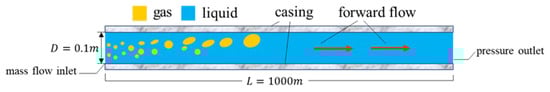
Figure 4. Schematic diagram of numerical simulation calculation area.

Table 1. Numerical simulation condition settings.

Parameters		Conditions
General	Length	1000 m
	Diameter	0.1 m
	Endtime	10,000 s
	Maxdt	5 s
	Mindt	0.001 s
	Sections	1000
Boundary	Inlet	Water mass flow: 7.854 kg/s
	Inlet	Methane mass flow: 0.55 kg/s
	Outlet	Pressure outlet: 0.5 MPa–2.5 MPa
	Wall	Roughness: 0.00005 m

In order to avoid the huge difference in data magnitude causing the small-scale data to be submerged and the model accuracy to decrease, this paper uses the z-score standard normalization to normalize the data set, namely:

$$y^{\ast }={\displaystyle \frac{y-\overline{y}}{\sigma }}$$

(25)

where y is the original data, $\overline{y}$ and $\sigma$ are the mean and standard deviation of y, respectively, and $y^{\ast }$ is the processed data, whose mean and standard deviation are calculated based on the data of the simulation results.

4.2. Network Hyperparameter Selection and Loss Function Construction

Since the role of the trunk and branch networks is to find a vector function that makes Equation (22) true, the structures of these two networks can be arbitrarily selected, such as fully connected neural network (FCN), convolutional neural network (CNN), etc. This paper first selects the CNN + FCN structure, and then compares the calculation time and accuracy of different structures. The specific parameters are shown in Table 2.

Table 2. Summary of network parameters.

Feature	CNN (Branch)	FCN (Trunk)
Input Dimension	4 channels × 101 points	2D coordinates
Network Depth	4 layers	4 layers
Hidden Units	32 channels	64 units
Output Dimension	256 units	64 units
Activation Function	ReLU	ReLU

The loss function of this paper consists of two parts. The other part of the loss function is the loss of the control equation. This paper adopts the drift-flux model, and transforms the gas phase continuity equation, liquid phase continuity equation, gas–liquid two-phase mixed momentum equation and drift velocity equation into the following form after dimensionless and standard normalization:

$$L_1={\displaystyle \frac{1}{{\sigma }_t}}{\displaystyle \frac{𝜕}{𝜕t^{\ast }}}\left({{\alpha }_g\dot{\rho }}_g\right)+{\displaystyle \frac{1}{{\sigma }_z}}{\displaystyle \frac{𝜕}{𝜕z^{\ast }}}\left({{\alpha }_g\dot{\rho }}_g{\dot{v}}_g\right)$$

(26)

$$L_2={\displaystyle \frac{1}{{\sigma }_t}}{\displaystyle \frac{𝜕}{𝜕t^{\ast }}}\left({{\alpha }_l\dot{\rho }}_l\right)+{\displaystyle \frac{1}{{\sigma }_z}}{\displaystyle \frac{𝜕}{𝜕z^{\ast }}}\left({{\alpha }_l\dot{\rho }}_l{\dot{v}}_l\right)$$

(27)

$$L_3={\displaystyle \frac{1}{{\sigma }_t}}{\displaystyle \frac{𝜕}{𝜕t^{\ast }}}\left({{\alpha }_g\dot{\rho }}_g{\dot{v}}_g+{\alpha }_l{\dot{\rho }}_l{\dot{v}}_l\right)+{\displaystyle \frac{1}{{\sigma }_z}}{\displaystyle \frac{𝜕}{𝜕z^{\ast }}}\left({{\alpha }_g\dot{\rho }}_g{\dot{v}}_g^2+{\alpha }_l{\dot{\rho }}_l{\dot{v}}_l^2+\dot{p}\right)-{\displaystyle \frac{F_w+{\rho }_{m}gsin\theta }{{\rho }_{m_i}{v}_{m_i}^2/H}}$$

(28)

$$L_4={\dot{v}}_g-{C_0\dot{v}}_m-v_d$$

(29)

Among them, ${\dot{\alpha }}_g,{\dot{v}}_g,{\dot{v}}_l,\dot{p}$ are the predicted values of the neural network output, ${\rho }_{m_i},v_{mi}$, vmi are calculated according to the inlet boundary conditions, $t^{\ast }and{z}^{\ast }$ are the coordinates after standard normalization, and ${\sigma }_t$, ${\sigma }_z$ are their respective standard deviations. The total physical loss function is expressed as:

$$L_{physics}={\displaystyle \frac{1}{N_c}}\sum _{k=1}^{N_c}\left({\omega }_1{\left|L_1^{\left(k\right)}\right|}^2+{\omega }_2{\left|L_2^{\left(k\right)}\right|}^2+{\omega }_3{\left|L_3^{\left(k\right)}\right|}^2+{\omega }_4{\left|L_4^{\left(k\right)}\right|}^2\right)$$

(30)

Among them, $N_c$ represents the number of configuration points in the neural network, and the mean square error loss (MSE) function is used here. The other part is data loss. In data loss, the predicted value output by the neural network is compared with the data ${\dot{\alpha }}_{g_{data}},{\dot{v}}_{g_{data}},{\dot{v}}_{l_{data}},{\dot{p}}_{data}$ after standard normalization. The specific form is:

$$L_{Data}={\displaystyle \frac{1}{N}}\sum _{i=1}^N({\omega }_5|{\dot{v}}_{g_{data}}^{\left(i\right)}-{\dot{v}}_g^{\left(i\right)}{|}^2+{\omega }_6|{\dot{v}}_{l_{data}}^{\left(i\right)}-{\dot{v}}_l^{\left(i\right)}{|}^2+{\omega }_7|{\dot{\alpha }}_{g_{data}}^{\left(i\right)}-{\dot{\alpha }}_g^{\left(i\right)}{|}^2+{\omega }_8|{\dot{p}}_{data}^{\left(i\right)}-{\dot{p}}^{\left(i\right)}{|}^2)$$

(31)

${\omega }_5,{\omega }_6,{\omega }_7,{\omega }_8$ are the weights of the losses of each part. It was observed that even after normalization, the magnitude of the pressure loss term was consistently two orders larger than the other terms. To prevent the total loss from being dominated by this single term and to ensure a balanced optimization process where all physical constraints are learned effectively, the weight ${\omega }_8$ is set to 0.01. This intentionally scales all loss components to a comparable order of magnitude. The total loss function is expressed as:

$$L_{total}=L_{Data}+L_{physics}$$

(32)

4.3. Results Analysis

First, the Adam optimizer was used, the learning rate was set to 0.001, and the training was performed for 10,000 steps. The training loss curve is shown in Figure 5. As the number of training times increases, the total loss decreases more and more slowly. Some of the results on the test set after training are shown in Figure 6. The first line is the OLGA data value, the second line is the model prediction value, and the third line is the error distribution cloud map. Each column is the distribution cloud map of gas content, gas absolute velocity, liquid absolute velocity, and pressure. The mean relative error (MRE) is used here for display. As can be seen from the figure, the results predicted by the deep operator network model are basically consistent with the simulation results of OLGA. A closer inspection of the error cloud maps in Figure 6 reveals a more nuanced performance. While the overall agreement is excellent, the largest relative errors are predominantly concentrated near the inlet (dimensionless position ≈ −1.5) and, to a lesser extent, the outlet of the wellbore. This phenomenon is likely attributable to two factors: First, the inlet and outlet represent boundary conditions where significant physical gradients in velocity and void fraction occur, making these regions inherently more challenging for the neural network to approximate with high fidelity. Second, the flow profile near the inlet may not be fully developed, introducing complex local dynamics that are more difficult to capture compared to the more stable flow in the middle section of the pipe. Nevertheless, even in these challenging regions, the absolute error remains small, demonstrating the robustness of the model. The deep operator network model can effectively simulate the flow field distribution under different pressure outlet conditions.

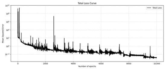
Figure 5. Training loss curve.

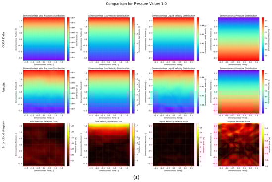
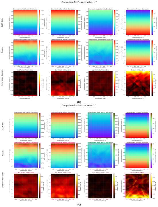
Figure 6. Comparison of PI-DeepONet model and OLGA data results under different outlet pressure conditions. (a) $p_{out}=1.0\mathrm{M}\mathrm{P}\mathrm{a}$, (b) $p_{out}=1.7\mathrm{M}\mathrm{P}\mathrm{a}$, (c) $p_{out}=2.2\mathrm{M}\mathrm{P}\mathrm{a}$.

Figure 7 shows the performance of the model on the test set. It can be seen from the figure that in the five test conditions, the maximum average relative error of a single condition is within 2.6%; in the overall situation, the maximum average relative error is the gas content distribution, which is within 1.8%, and the minimum average relative error is the pressure distribution, which is within 0.2%. It is noteworthy from Figure 7 that the pressure distribution consistently yields the lowest prediction error (within 0.2%). This high accuracy is likely because the pressure field along the horizontal wellbore is relatively smooth and varies monotonically, making it easier for the model to learn the underlying operator. Conversely, the gas velocity and void fraction exhibit slightly higher errors. This is expected, as these parameters are more sensitive to local two-phase flow dynamics and can exhibit more complex, non-linear behavior, which poses a greater challenge for the learning algorithm. The average relative error of the four parameters is 0.925%, indicating that the deep operator network model has a good performance on the test set and can effectively predict the flow field distribution under different conditions.

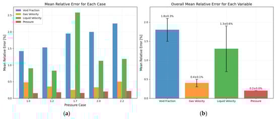
Figure 7. Statistics of average relative error (a) Average relative error of each case (b) Average relative error of all cases.

Figure 8 shows the performance of PI-DeepONet under different hyperparameters. Different network structures, different numbers of network layers, and different learning rates are used here, and the same neural network width of 64 is used. As can be seen from the figure, the network structure is the key factor affecting the performance of the model. The mean relative error (MRE) of the model using the FCN + FCN structure is significantly lower than that of the model using the CNN + FCN structure. The choice of learning rate is also crucial. When the learning rate is set to a higher 0.01, the MRE of the model is at a high level regardless of the network structure or number of layers (as shown by the dark purple line in the figure). On the contrary, lower learning rates (0.001 and 0.005) are more likely to obtain ideal performance. The best results in the figure (yellow and green lines) appear under these two learning rate settings. Under the premise of the optimal FCN + FCN structure and low learning rate, the network depth also shows a clear impact. When both the Branch network and the Trunk network are set to 3 layers, the performance of the model is generally better than that of the case with 1 or 2 layers.

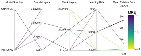
Figure 8. Comparison of model performance under different hyperparameter combinations.

Table 3 shows the performance of the model under different network widths when the FCN + FCN network structure is used and the number of network layers is 3. It can be seen from the table that when the width is 64, the average relative error is within 1%, and the calculation time is moderate. Although the accuracy is slightly improved when the width is 128, the computing resources consumed are 1.5 times that of the former, and the computing efficiency is reduced.

Table 3. Performance under different network widths.

Network Width	Mean Relative Error (%)	Training Time (h)
16	2.25	4
32	0.45	4.6
64	0.38	5
128	0.25	7.5

In summary, the optimal hyperparameter combination in this experiment is: using FCN + FCN network structure, 3 layers for both Branch and Trunk networks, 64 network width, and using a learning rate of 0.001. At this time, the model achieved the lowest average relative error of 0.375%.

In addition, this paper also compares the time consumption of the 5 cases tested. All tests were performed using an NVIDIA RTX 4090 GPU (NVIDIA Corporation, Santa Clara, CA, USA) and AMD Ryzen 7 9700X 8-Core Processor CPU (Advanced Micro Devices, Inc., Santa Clara, CA, USA). As shown in Table 4, the test time cost of using the deep operator model is less than 0.1 s, and the calculation speed of PI-DeepONet is significantly faster than the OLGA numerical simulation. That is, after training, the model can achieve fast calculation of different working conditions. It is important to contextualize this comparison of computation times. This comparison is not intended as a direct, hardware-normalized benchmark, but rather to highlight the fundamental difference in computational paradigms. Industrial simulators like OLGA are primarily designed for high-accuracy physical modeling on CPU architectures and are not typically optimized for the massive parallelism offered by GPUs. In contrast, our deep learning approach inherently leverages GPU acceleration for rapid inference. Thus, the dramatic speed-up demonstrates the transformative potential of switching the computational paradigm for applications where real-time performance is paramount.

Table 4. Comparison of computation time between PI-DeepONet and OLGA.

Experiment	OLGA (s)	PI-DeepONet (s)
Case1–5	5200	0.1

In order to verify the performance of this model in the case of missing data, the method of randomly hiding data is adopted. 10% of the time point data are randomly selected for hiding in each working condition; that is, all the data at the selected time points do not appear in the data loss function. This paper selects the same 20 working conditions as before for training, and adopts the three-layer FCN + FCN network structure with better performance. The results of comparing the predicted values and true values of the hidden point data of some working conditions are shown in Figure 9, and the average results of all working condition data are shown in Figure 10.

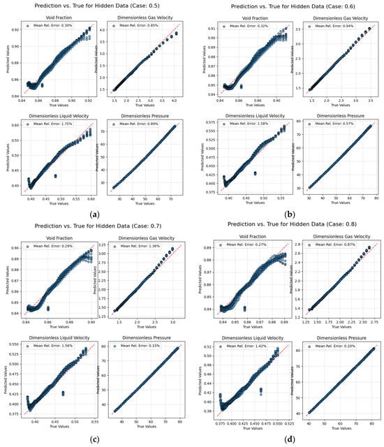
Figure 9. Results of some operating data points. (a) $p_{out}=0.5\mathrm{M}\mathrm{P}\mathrm{a}$, (b) $p_{out}=0.6\mathrm{M}\mathrm{P}\mathrm{a}$, (c) $p_{out}=0.7\mathrm{M}\mathrm{P}\mathrm{a},($d) $p_{out}=0.8\mathrm{M}\mathrm{P}\mathrm{a}$.

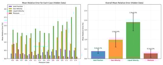
Figure 10. Average results for all cases.

As shown in Figure 10, the maximum relative average error of a single condition is 1.9%, and the average relative error of the overall condition is 0.9%, indicating that the model can still perform well when some points are accurate. The performance of the model when 20% to 80% of the data points are hidden is subsequently explored, as shown in Table 5.

Table 5. Performance when hiding different percentages of data.

Hidden Data Ratio (%)	Mean Relative Error on Hidden Data (%)	Mean Relative Error on the Test Set (%)
20	0.88	1.05
30	0.65	0.78
40	1.18	1.23
50	0.98	1.00
60	1.53	1.53
70	1.68	1.98
80	4.30	4.65

The first column of Table 5 is the percentage of hidden data, the second column is the relative average error of predicting hidden data, and the third column is the relative average error on the test set. When less than 50% of the data is hidden, the average relative error of the model is also around 1%, which is at a very low level. When more than 70% of the data is hidden, the prediction results of the model have a significant drop, but still remain within 5%. This shows that when a large amount of data is missing, the model can still have the ability to predict through the constraints of its internal control equations and the remaining small amount of data.

5. Conclusions

This paper proposes a fast calculation method for two-phase flow in horizontal gas wells based on PI-DeepONet, and the following conclusions are obtained:

• By embedding the physical laws of the drift-flux model directly into the deep operator network, this study presents a novel approach that effectively overcomes the reliance on large-scale data, a common limitation of purely data-driven methods. This physics-informed strategy enables high prediction accuracy even with sparse training data. The model demonstrated excellent performance, with an average relative error controlled to within 1% across multiple test cases, which is a significant improvement over traditional deep learning models in data-scarce scenarios.
• The practical engineering value of this method is highlighted by its remarkable computational efficiency. When benchmarked against the industry-standard simulator (OLGA), the trained PI-DeepONet model completes a full-field prediction in under 0.1 s, representing a computational speed-up of nearly 50,000 times. This transformative performance makes the model highly suitable for real-world applications that demand immediate feedback.
• The experimental results also provide clear guidance for the model’s implementation. An optimal setup was identified using an FCN + FCN network structure with 3 layers, a network width of 64, and a learning rate of 0.001, offering a solid baseline for researchers aiming to replicate this work. Furthermore, the model’s robustness was demonstrated by its ability to perform well even when a significant portion of the training data was hidden, underscoring the power of integrating physical constraints into the learning process.
• Even when hiding up to 80% of the real data, the model still has relatively good expressiveness, with a relative average error of less than 5% on the test set, and can be used in situations where some data is missing in actual working conditions.

While this study provides a strong foundation, its limitations also point toward important future research. The current model is based on a one-dimensional framework and was validated exclusively on data generated by numerical simulations. Therefore, the immediate and most critical next step is to apply and test this method using real-world data from field operations. Future work should also focus on extending the model to handle more complex scenarios, such as two-dimensional or three-dimensional simulations, and studying its stability under a wider range of physical conditions, including changing phase compositions and more dynamic flow regimes. Future studies could also further enhance the statistical robustness of the validation by employing more extensive schemes, such as k-fold cross-validation. Subsequent work will also continue to explore the optimization of the network architecture and hyperparameters for other specific physical problems.

References

- Omotoye, G.B.; Bello, B.G.; Tula, S.T.; Kess-Momoh, A.J.; Daraojimba, A.I.; Adefemi, A. Navigating global energy markets: A review of economic and policy impacts. Int. J. Sci. Res. Arch. 2024, 11, 195–203. [Google Scholar] [CrossRef]
- Wang, J.; Guo, Q.; Zhao, C.; Wang, Y.; Yu, J.; Liu, Z.; Chen, N. Potentials and prospects of shale oil-gas resources in major basins of China. Acta Pet. Sin. 2023, 44, 2033–2044. [Google Scholar] [CrossRef]
- Lei, Q.; Xu, Y.; Cai, B.; Guan, B.; Wang, X.; Bi, G.; Li, H.; Li, S.; Ding, B.; Fu, H.; et al. Progress and prospects of horizontal well fracturing technology for shale oil and gas reservoirs. Pet. Explor. Dev. 2022, 49, 191–199. [Google Scholar] [CrossRef]
- Duan, Y.; Zhu, Z.; He, H.; Xuan, G.; Yu, X. Simulation of Two-Phase Flowback Phenomena in Shale Gas Wells. Fluid Dyn. Mater. Process. 2024, 20, 349–364. [Google Scholar] [CrossRef]
- Obi, C.; Hasan, A.; Rahman, M.; Banerjee, D. Multiphase flow challenges in drilling, completions, and injection: Part 1. Petroleum 2024, 10, 557–569. [Google Scholar] [CrossRef]
- Su, Y.; Ma, H.; Guo, J.; Shen, X.; Yang, Z.; Wu, J. The behaviors of gas-liquid two-phase flow under gas kick during horizontal drilling with oil-based muds. Petroleum 2024, 10, 49–67. [Google Scholar] [CrossRef]
- Zhou, X.; Zhang, L.; Qi, J.; Wang, Y.; Zhang, K.; Zhang, R.; Sun, Y. Integrated wellbore-surface pressure control production optimization for shale gas wells. Nat. Gas Ind. B 2025, 12, 123–134. [Google Scholar] [CrossRef]
- Talebi, S.; Kazeminejad, H.; Davilu, H. A numerical technique for analysis of transient two-phase flow in a vertical tube using the drift flux model. Nucl. Eng. Des. 2012, 242, 316–322. [Google Scholar] [CrossRef]
- Wei, N.; Xu, C.; Meng, Y.; Li, G.; Ma, X.; Liu, A. Numerical simulation of gas-liquid two-phase flow in wellbore based on drift flux model. Appl. Math. Comput. 2018, 338, 175–191. [Google Scholar] [CrossRef]
- Hajizadeh, A.; Kazeminejad, H.; Talebi, S. Formulation of a fully implicit numerical scheme for simulation of two-phase flow in a vertical channel using the Drift-Flux Model. Prog. Nucl. Energy 2018, 103, 91–105. [Google Scholar] [CrossRef]
- Liu, C.; Zhou, G.; Shyy, W.; Xu, K. Limitation principle for computational fluid dynamics. Shock Waves 2019, 29, 1083–1102. [Google Scholar] [CrossRef]
- Xu, B.; Zhang, X.; Wang, Y.; Liu, W.; Meng, Z. Self-adaptive physical information neural network model for prediction of two-phase flow annulus pressure. Acta Pet. Sin. 2023, 44, 545. [Google Scholar] [CrossRef]
- Taye, M.M. Understanding of machine learning with deep learning: Architectures workflow, applications and future directions. Computers 2023, 12, 91. [Google Scholar] [CrossRef]
- Song, Z.; Zou, S.; Zhou, W.; Huang, Y.; Shao, L.; Yuan, J.; Gou, X.; Jin, W.; Wang, Z.; Chen, X.; et al. Clinically applicable histopathological diagnosis system for gastric cancer detection using deep learning. Nat. Commun. 2020, 11, 4294. [Google Scholar] [CrossRef]
- Kabir, H.; Wu, J.; Dahal, S.; Joo, T.; Garg, N. Automated estimation of cementitious sorptivity via computer vision. Nat. Commun. 2024, 15, 9935. [Google Scholar] [CrossRef]
- Raissi, M.; Perdikaris, P.; Karniadakis, G.E. Physics-informed neural networks: A deep learning framework for solving forward and inverse problems involving nonlinear partial differential equations. J. Comput. Phys. 2019, 378, 686–707. [Google Scholar] [CrossRef]
- Lu, L.; Jin, P.; Pang, G.; Zhang, Z.; Karniadakis, G.E. Learning nonlinear operators via DeepONet based on the universal approximation theorem of operators. Nat. Mach. Intell. 2021, 3, 218–229. [Google Scholar] [CrossRef]
- Koric, S.; Abueidda, D.W. Data-driven and physics-informed deep learning operators for solution of heat conduction equation with parametric heat source. Int. J. Heat Mass Transf. 2023, 203, 123809. [Google Scholar] [CrossRef]
- Mao, Z.; Lu, L.; Marxen, O.; Zaki, T.A.; Karniadakis, G.E. DeepM&Mnet for hypersonics: Predicting the coupled flow and finite-rate chemistry behind a normal shock using neural-network approximation of operators. J. Comput. Phys. 2021, 447, 110698. [Google Scholar] [CrossRef]
- Wang, S.; Wang, H.; Perdikaris, P. Learning the solution operator of parametric partial differential equations with physics-informed DeepONets. Sci. Adv. 2021, 7, eabi8605. [Google Scholar] [CrossRef]
- Zuber, N.; Findlay, J.A. Average volumetric concentration in two-phase flow systems. J. Heat Transf. 1965, 87, 453–468. [Google Scholar] [CrossRef]
- Wallis, G.B. One-Dimensional Two-Phase Flow; Courier Dover Publications: New York, NY, USA, 2020. [Google Scholar]
- Ishii, M. One-Dimensional Drift-Flux Model and Constitutive Equations for Relative Motion Between Phases in Various Two-Phase Flow Regimes (No. ANL-77-47); Argonne National Lab.: Lemont, IL, USA, 1977. [CrossRef]
- Shi, H.; Holmes, J.A.; Diaz, L.R.; Durlofsky, L.J.; Aziz, K. Drift-flux parameters for three-phase steady-state flow in wellbores. SPE J. 2005, 10, 130–137. [Google Scholar] [CrossRef]
- Bhagwat, S.M.; Ghajar, A.J. A flow pattern independent drift flux model based void fraction correlation for a wide range of gas–liquid two phase flow. Int. J. Multiph. Flow 2014, 59, 186–205. [Google Scholar] [CrossRef]
- Chen, T.; Chen, H. Universal approximation to nonlinear operators by neural networks with arbitrary activation functions and its application to dynamical systems. IEEE Trans. Neural Netw. 1995, 6, 911–917. [Google Scholar] [CrossRef] [PubMed]
- He, J.; Koric, S.; Abueidda, D.; Najafi, A.; Jasiuk, I. Geom-deeponet: A point-cloud-based deep operator network for field predictions on 3d parameterized geometries. Comput. Methods Appl. Mech. Eng. 2024, 429, 117130. [Google Scholar] [CrossRef]
- Xu, C.; Cao, B.T.; Yuan, Y.; Meschke, G. A multi-fidelity deep operator network (DeepONet) for fusing simulation and monitoring data: Application to real-time settlement prediction during tunnel construction. Eng. Appl. Artif. Intell. 2024, 133, 108156. [Google Scholar] [CrossRef]
- Lim, D.G.; Lee, G.Y.; Park, Y.H. Application of DeepONet to predict transient drop motion of the control rod in real-time. Nucl. Eng. Technol. 2025, 57, 103620. [Google Scholar] [CrossRef]
- Yang, Y. Deeponet for solving PDEs: Generalization analysis in Sobolev training. arXiv 2024, arXiv:2410.04344. [Google Scholar] [CrossRef]
- Kopaničáková, A.; Karniadakis, G.E. Deeponet based preconditioning strategies for solving parametric linear systems of equations. SIAM J. Sci. Comput. 2025, 47, C151–C181. [Google Scholar] [CrossRef]
- Xu, W.; Lu, Y.; Wang, L. Transfer learning enhanced deeponet for long-time prediction of evolution equations. In Proceedings of the AAAI Conference on Artificial Intelligence, Washington DC, USA, 7–14 February 2023; Volume 37, pp. 10629–10636. [Google Scholar] [CrossRef]
Disclaimer/Publisher’s Note: The statements, opinions and data contained in all publications are solely those of the individual author(s) and contributor(s) and not of MDPI and/or the editor(s). MDPI and/or the editor(s) disclaim responsibility for any injury to people or property resulting from any ideas, methods, instructions or products referred to in the content. |
© 2025 by the authors. Licensee MDPI, Basel, Switzerland. This article is an open access article distributed under the terms and conditions of the Creative Commons Attribution (CC BY) license (https://creativecommons.org/licenses/by/4.0/).