Article

Ternary Precursor Centrifuge Rolling Bearing Fault Diagnosis Based on Adaptive Sample Length Adjustment of 1DCNN-SeNet

1
Quzhou College of Technology, Quzhou 324000, China
2
College of Communication Engineering, Jilin University, Changchun 130022, China
3
Quzhou Special Equipment Inspection Center, Quzhou 324000, China
*
Authors to whom correspondence should be addressed.
Processes 2024, 12(4), 702; https://doi.org/10.3390/pr12040702
Submission received: 29 February 2024 / Revised: 23 March 2024 / Accepted: 26 March 2024 / Published: 29 March 2024

Abstract

:
To address the issues of uneven sample lengths in the centrifuge machine bearings of the ternary precursor, inaccurate fault feature extraction, and insensitivity of important feature channels in rolling bearings, a rolling bearing fault diagnosis method based on adaptive sample length adjustment of one-dimensional convolutional neural network (1DCNN) and squeeze-and-excitation network (SeNet) is proposed. Firstly, by controlling the cumulative variance contribution rate in the principal component analysis algorithm, adaptive adjustment of sample length is achieved, reducing data with uneven sample lengths to the same dimensionality for various classes. Then, the 1DCNN extracts local features from bearing signals through one-dimensional convolution-pooling operations, while the SeNet network introduces a channel attention mechanism which can adaptively adjust the importance between different channels. Finally, the 1DCNN-SeNet model is compared with four classic models through experimental analysis on the CWRU bearing dataset. The experimental results indicate that the proposed method exhibits high diagnostic accuracy in rolling bearings, demonstrating good adaptability and generalization capabilities.

1. Introduction

As a critical component of mechanical equipment, rolling bearings are responsible for supporting and transmitting the forces of rotating components, ensuring the normal operation of mechanical systems [1,2,3]. In the operation of the ternary precursor filtering and washing centrifuge, rolling bearings play a crucial role, facing numerous challenges due to high-intensity operations and complex working conditions. Firstly, rolling bearings typically operate in complex and extreme environments, such as high temperatures, high speeds, and high pressures, imposing extremely high requirements on the durability and stability of the bearings. Secondly, heavy equipment loads can subject bearings to tremendous pressure, leading to wear, fatigue, corrosion, and deformation over prolonged periods [4,5,6]. Bearing damage can lead to unstable operation of equipment [7], thereby affecting the performance and efficiency of the entire system. In crucial sectors such as aerospace, automotive, and manufacturing industries, bearing failures can pose serious threats to safety, potentially causing casualties and property damage. Bearings need to face challenges such as higher wear resistance, corrosion, and high temperature resistance [8,9,10], and to overcome the challenges of rolling bearings, engineers are incorporating new materials and innovative technologies such as environmental seals in the manufacture of bearings. For instance, effective sealing designs can prevent external substances like dust and moisture from entering the bearing, thus reducing the occurrence of wear-related failures. Therefore, timely detection and repair of rolling bearing faults are crucial for preventing equipment downtime and damage, reducing maintenance costs, and enhancing productivity.
Due to the presence of multiple frequency components and complex time-varying characteristics in bearing signals, which exhibit nonlinear and non-stationary properties, traditional linear analysis methods have certain limitations in fault diagnosis. To address this issue, numerous scholars have conducted extensive research and widely applied nonlinear signal processing techniques and machine learning algorithms, such as wavelet transform [11,12], adaptive filtering, time-frequency analysis [13], support vector machines (SVMs) [14], and artificial neural networks (ANNs) [15]. In literature [16], features of the data are extracted through discrete Fourier transform, then the parameters in the support vector machine are optimized using the Bayesian algorithm, and finally fault diagnosis classification is completed using the reconstructed support vector machine. In literature [17], four types of information entropy are fused using the method of n-dimensional feature parameter distance, thereby completing the diagnosis of rolling bearing faults using the fusion entropy method. In literature [18], genetic algorithms are used to achieve optimal parameter values for weight parameters in artificial neural networks, and then mechanical bearing health diagnosis is completed using artificial neural networks. In literature [19], weighted least squares support vector machines are used for signal preprocessing, and then representative intrinsic mode functions containing fault information are selected using empirical mode decomposition for demodulation, thus completing fault feature recognition. In literature [20], the original vibration signal is adaptively decomposed into different frequency bands of Intrinsic Mode Functions (IMFs) using Empirical Mode Decomposition (EMD) integrated with Ensemble Empirical Mode Decomposition (EEMD). Subsequently, the IMFs are organized into angular domains using Envelope Order Tracking. Finally, a fault-sensitive matrix is established to accomplish the ultimate fault diagnosis task. On the one hand, these research findings provide some new insights for bearing fault diagnosis. On the other hand, with the development of intelligence, bearing fault diagnosis has also ushered in new opportunities and challenges. Among the methods mentioned above, manual extraction of features from vibration data is required, which is not only labor-intensive and complex but also susceptible to subjective factors.
The emergence of deep learning methods has provided a new approach for modeling and fault diagnosis of complex nonlinear systems. It automatically extracts key features from raw data and discovers potential fault features, thus achieving more precise fault diagnosis. In literature [21], the dimensionality of the original signals is reduced using principal component analysis algorithm, followed by fault classification and diagnosis using deep belief networks, without the need for complex signal processing. In literature [22], one-dimensional bearing signals are transformed into two-dimensional images through Markov transition field encoding, and then feature extraction and fault diagnosis are automatically performed using convolutional neural networks. In literature [23], a CNN-BiLSTM method for bearing fault diagnosis is proposed. Attention mechanisms, DropConnect, and Dropout are utilized to control the diagnostic effectiveness of the model. Literature [24] employs evolutionary algorithms to optimize generative adversarial networks, enhancing the fault recognition capability of the network through adversarial learning mechanisms to optimize the generator and discriminator. In literature [25], frequency features are extracted from vibration signals using the Generalized Demodulation Algorithm. Subsequently, 1D Convolutional Neural Networks (1DCNNs) are employed for fault classification and identification of the health status of rolling bearings. This method aims to minimize identification errors and enhance stability. The application of deep learning methods enables more accurate and efficient diagnosis of bearing health status, driving the widespread application and development of intelligent fault diagnosis in the industrial field. Therefore, this paper proposes a diagnostic method based on adaptive sample length adjustment of 1DCNN-SeNet, which exhibits better adaptability to bearing fault diagnosis tasks, deeply mines hidden fault information, and achieves more precise intelligent fault diagnosis. Its application in practical industrial fields is of significant importance.
This paper makes three main contributions:
(1)
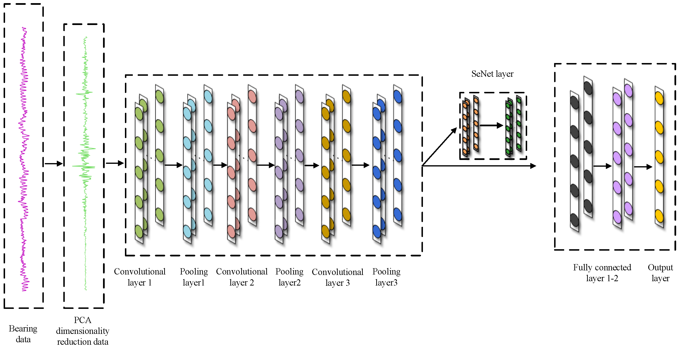
Adaptive adjustment based on the cumulative variance explained ratio in the Principal Component Analysis (PCA) algorithm reduces the data to a uniform dimensionality, addressing the issue of uneven sample lengths. This ensures effective fault diagnosis on input signals of different lengths.
(2)
We propose a fault diagnosis method called 1DCNN-SeNet, which leverages 1DCNN to automatically extract local feature information from the data and then utilizes SeNet to adaptively adjust the importance of each channel. This approach significantly enhances diagnostic accuracy and demonstrates distinct advantages.
(3)
A comparative analysis between the proposed method and four classical algorithms demonstrates that the proposed method outperforms in adapting to complex fault scenarios in rolling bearing fault diagnosis tasks. The analysis of accuracy curves, loss curves, and confusion matrices confirms the effectiveness and generalization capability of the proposed algorithm.

2. Research Objectives and Methodology Theory

2.1. Research Objectives

In the domain of bearing fault diagnosis, the research objective of this paper is to enhance the accuracy and reliability of bearing fault diagnosis by applying the PCA algorithm and the 1DCNN-SeNet fault diagnosis model. This is achieved through adaptive adjustment and feature extraction of bearing data, aiming to improve the accuracy and reliability of bearing fault diagnosis. Firstly, by applying the PCA algorithm, the issue of unevenness in bearing data samples is addressed, ensuring effective diagnosis can be conducted on signals of varying lengths. Secondly, leveraging the 1DCNN-SeNet model enables automatic extraction of local feature information from bearing data and adaptive adjustment of the importance of each channel, thereby better capturing fault characteristics. This provides more effective technical support for bearing fault diagnosis and maintenance, reducing the impact of mechanical faults on production and equipment operation, and enhancing production efficiency and equipment reliability.

2.2. Principal Component Analysis Algorithm

PCA [26,27], as a powerful tool for data processing and analysis, can transform high-dimensional data into low-dimensional data while extracting the main features of the data. By reducing dimensionality and extracting features from data, we can better understand the data, discover potential fault data information, and accelerate the speed of data processing and analysis. Therefore, using PCA for dimensionality reduction and feature extraction on bearing signals can effectively reduce the complexity and redundancy of the data, thus improving the speed and accuracy of bearing fault diagnosis.
In this paper, the PCA algorithm is employed to reduce bearing datasets of varying dimensions to a unified dimensionality while preserving the most significant fault feature information. Assuming a bearing dataset of a certain class contains samples and features, it can be represented as an matrix, where its matrix expression is
X = x 11 x 12 x 1 n x 21 x 22 x 2 n x m 1 x m 2 x m n
The entire process involves mapping the matrix to a m × k matrix Y, where k < n . This requires finding a transformation matrix of size n × k such that each column of matrix Y is the projection of matrix X onto this direction. The matrix Z can be obtained through the following steps:
max Z tr ( Z T X T X Z )
s . t . Z T Z = I
where I represents the identity matrix, and tr ( · ) denotes the trace of a matrix. To combine Equations (2) and (3) for solving, we can use the method of Lagrange multipliers to transform them as follows:
max Z tr ( Z T X T X Z ) λ ( Z T Z I )
Differentiating Equation (4) with respect to the parameter Z, and setting its derivative to zero, the calculation results are as follows:
X T X Z = λ Z
From Equation (5), we can conclude that the eigenvectors of the covariance matrix X T X are the matrix Z, and its corresponding eigenvalues are λ . To obtain the final matrix Y, the eigenvalues obtained are sorted in descending order, and the top k eigenvectors corresponding to these eigenvalues are selected to form the basis matrix Z; Therefore, the reduced matrix Y can be obtained through the following operation:
Y = X Z

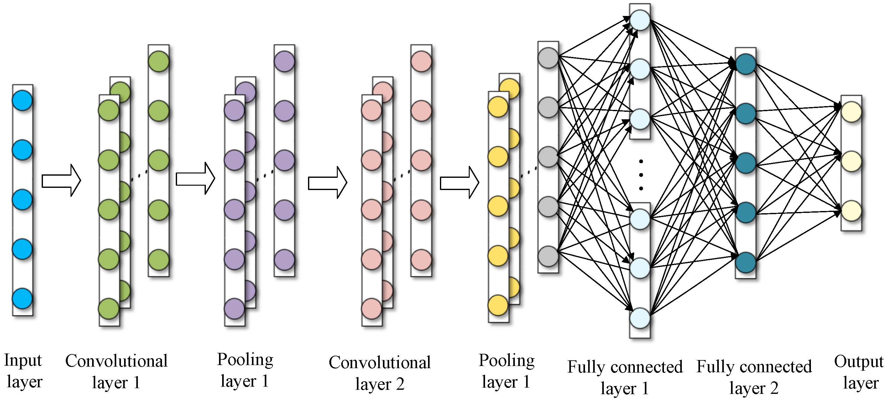
2.3. One-Dimensional Convolutional Neural Network

The 1DCNN possesses two important characteristics: local connectivity and weight sharing. Local connectivity enables automatic learning and extraction of local features from data, allowing for the neural network to handle large-scale data and improve computational efficiency. Weight sharing significantly reduces the number of parameters that need to be learned in the diagnostic model, thereby enhancing training efficiency and generalization capability. This enables the diagnostic model to handle various types of complex data. The basic structure of a 1DCNN is illustrated in Figure 1, consisting primarily of an input layer, convolutional layers, pooling layers, fully connected layers, and an output layer [28,29].
The convolutional layer extracts features from bearing data using convolutional kernels. The kernels slide over the input bearing data, perform convolution operations, add the corresponding bias vectors, and finally the output feature vectors are processed through an activation function. The mathematical operations can be represented as
x j k = f ( i x i k 1 m i j k + b j k )
where x j k represents the output of the jth neuron in the kth layer of the network, f ( · ) denotes the corresponding activation function, x i k 1 is the output of the ith neuron in the k 1 th layer of the network, m i j k represents the convolutional kernel corresponding to the kth layer, and b j k is the bias vector corresponding to the kth layer.
The pooling layer typically follows the convolutional layer. It performs downsampling operations on the local features learned by the convolutional layer, compressing the local feature information into a smaller representation. This reduces the number of parameters that need to be learned in subsequent network layers, removes redundant information, and retains important feature information, thereby enhancing the overall learning efficiency of the model. The mathematical operations can be represented as
h j k = max ( i 1 ) S + 1 < t < i S g j k 1 ( t )
where h j k represents the output of the jth neuron in the kth layer of the network, S represents the size of the convolutional kernel in the pooling layer, and g j k 1 ( t ) represents the output of the k 1 th neuron in the jth feature vector of the tth layer.
The output of the pooling layer is flattened to convert it into a one-dimensional vector, which serves as the input to the fully connected layer. The fully connected layer learns weight parameters to associate these local features with the classification diagnosis task. The mathematical operations can be represented as
o ( x ) = f ( ω x + b )
where f ( · ) represents the corresponding activation function, w denotes the corresponding weight vector, b is the corresponding bias vector, and o represents the output of this layer.
The output layer generally uses the softmax function to produce the final diagnostic result. The mathematical operation can be represented as
y k = e a k i = 1 n e a i
where y k represents the output of the kth neuron, a k represents the kth input signal, and a i represents the ith input signal.

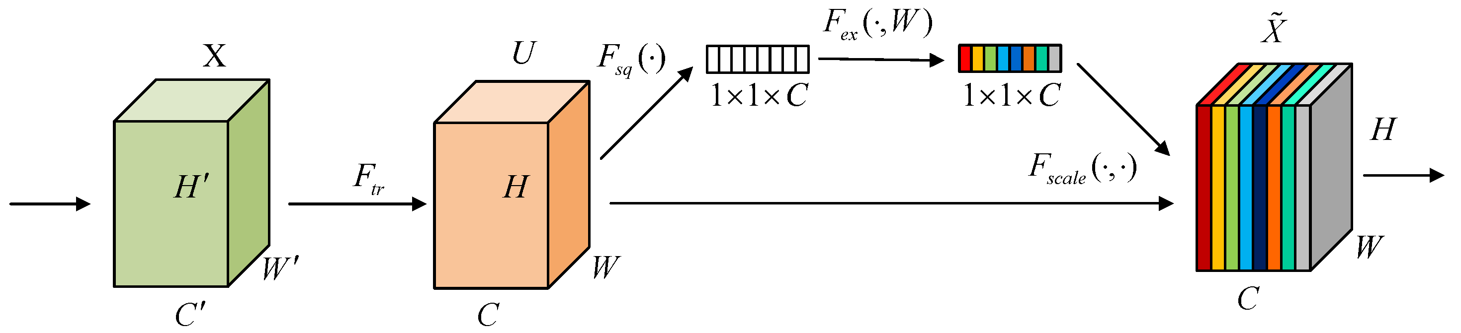
2.4. Squeeze-and-Excitation Network (SENet)

SENet [30] is a type of channel attention mechanism. By analyzing and processing the relationships between feature channels, it selectively learns important feature information and dynamically adjusts the dependencies between different feature channels in the convolutional neural network. This enables the diagnostic model to adaptively adjust the importance of each channel, suppress irrelevant channels, and effectively improve the diagnostic classification and representation capabilities of the model. The basic structure of the SENet is illustrated in Figure 2, primarily consisting of two important operations: squeeze and excitation [31,32].
From Figure 2, it can be seen that matrix U is obtained from matrix X through mapping transformation F t r using excitation function X R H × W × C , U R H × W × C , where H · W · C , and H · W · C represent the height, width, and number of channels of matrices X and U, respectively. The mathematical operations can be represented as
u i = v i × X = j = 1 C v i j × x j
where v i represents the ith convolutional kernel, u i represents the ith sub-matrix in matrix, v i j represents the jth input in the ith convolutional kernel, and x j ( i ) represents the jth input.
The squeeze operation involves global average pooling of matrix U, compressing the spatial dimensions of the feature maps in matrix U, along the H × W dimensions. This results in a single value representing global information aggregation obtained by averaging each channel, i.e., a one-dimensional feature vector 1 × 1 × C . The mathematical operation can be represented as
Z i = F s q ( u i ) = 1 H × W m = 1 H n = 1 W u i ( m , n )
where Z i represents the compressed feature of channel i and u i ( m , n ) represents the corresponding mapped value in the ith channel at the mth row and nth column.
The excitation operation primarily learns the nonlinear dependencies between the output feature channels of the squeeze operation. It further dynamically adjusts the importance weights of each channel, focusing more on important feature information. The excitation operation is composed of a lightweight fully connected sequence. The specific mathematical operations between its internal components can be represented as
s i = F e x ( Z , W ) = σ ( g ( Z , W ) ) = σ ( W 2 δ ( W 1 , Z ) )
W 1 R C q × C , W 2 R C × C q
where σ represents the ReLU activation function after dimension reduction, δ represents the Sigmoid activation function after dimension expansion, W 1 and W 2 are the parameters of the two fully connected layers, q is the scaling factor, and s i is the output of channel i after the excitation operation.
The output of the excitation operation is a channel-wise weight vector 1 × 1 × C , which integrates the importance weights of each channel. Finally, we need to perform element-wise multiplication between the channel weight vector and the original matrix U, which is referred to as the scale operation. The mathematical operation can be represented as
X ˜ = F s c a l e ( u i , s i ) = s i × u i
where X ˜ represents the final output feature map of the SENet network.

3. Experiment Validation and Result Analysis

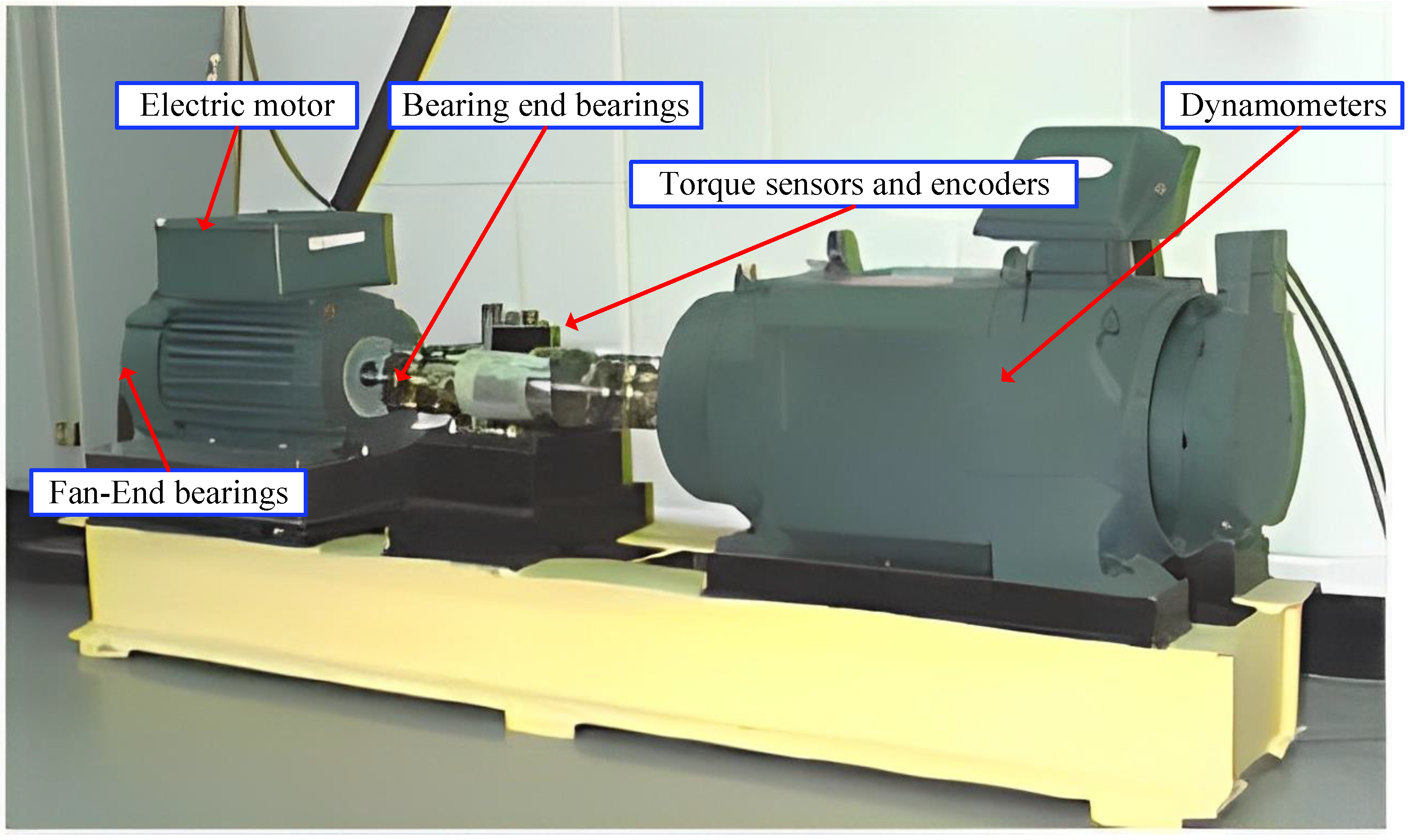
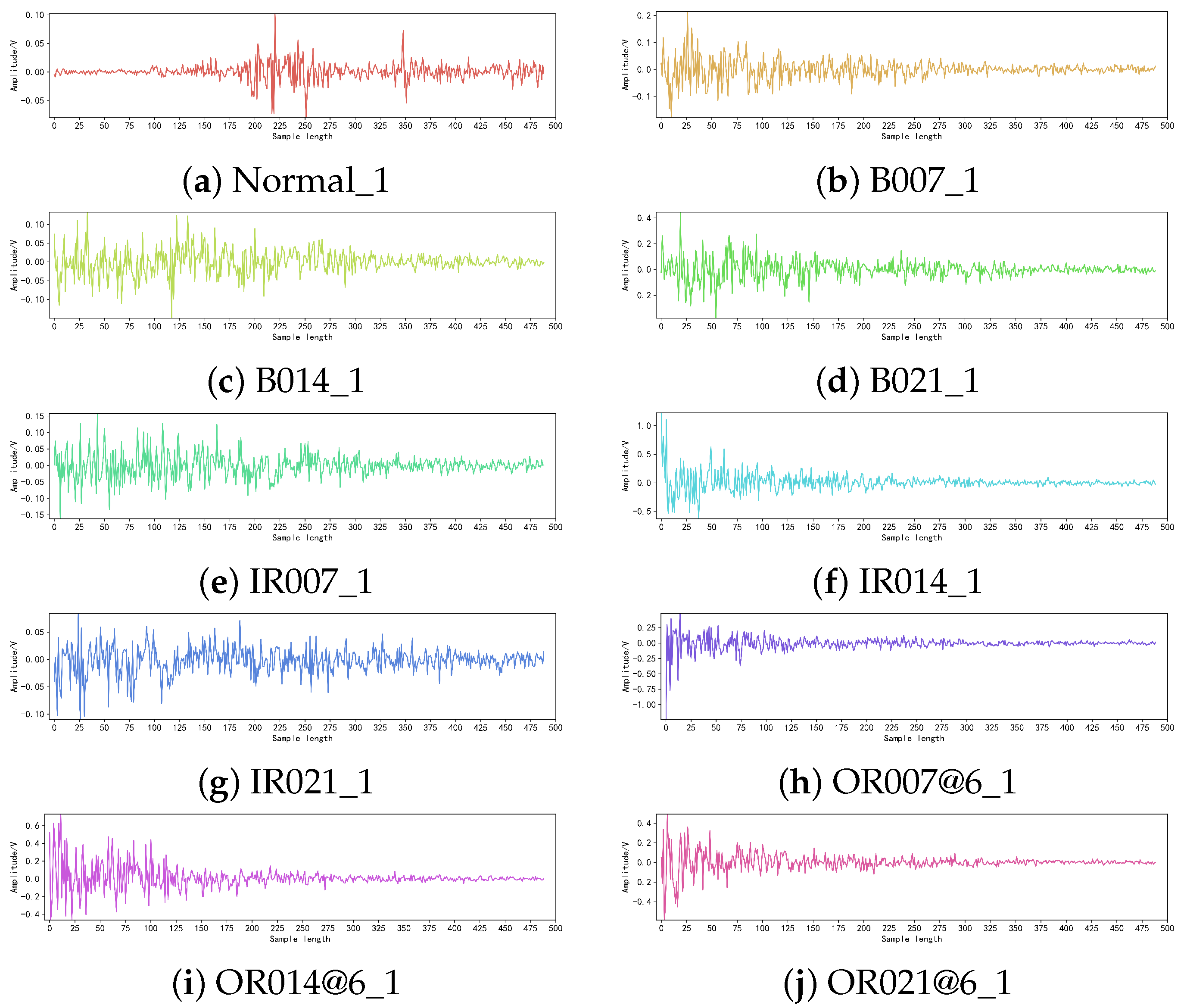
3.1. Description of Experimental Dataset

This study utilizes the publicly available bearing dataset provided by Case Western Reserve University (CWRU) [33] as the research subject. This dataset simulates various types and degrees of bearing faults, collecting a large amount of vibration signal data from sensors. The specific experimental bearing equipment is shown in Figure 3. The drive end fault data were selected from a deep groove ball bearing model 6205-2RS JEM SKF. The sampling frequency was set to 12 kHz, the motor load was 1 horsepower (HP), and the motor speed was approximately 1722 rpm. The vibration data were collected using accelerometer sensors connected to the magnetic base attached to the housing, while the speed and motor load in horsepower were measured by torque sensors and encoders, respectively. Bearing faults were machined using electrical discharge machining and classified into three damage diameters: 0.007 inches, 0.014 inches, and 0.021 inches. Four types of data were selected, representing inner race faults, outer race faults, roller faults, and normal operation of the bearings. The samples were divided into equal intervals, with cutting lengths of 1004, 1014, 1024, and 1034, resulting in four different sampling lengths for the original dataset. The specific details of the bearing original dataset are shown in Table 1, and the corresponding curves for 10 different operating conditions are shown in Figure 4.

3.2. Data Normalization Process

The original bearing dataset contains 10 different operating states. To better analyze and process these data, dimensional differences between categories are eliminated and the convergence speed of model training is accelerated. In this paper, we perform min–max normalization on the original bearing dataset. The bearing dataset is normalized. The specific mathematical operation can be represented as
y i = x i min 1 i n { x j } max 1 i n { x j } min 1 i n { x j }
where y i represents the normalized output of the new sequence, y i [ 0 , 1 ] .

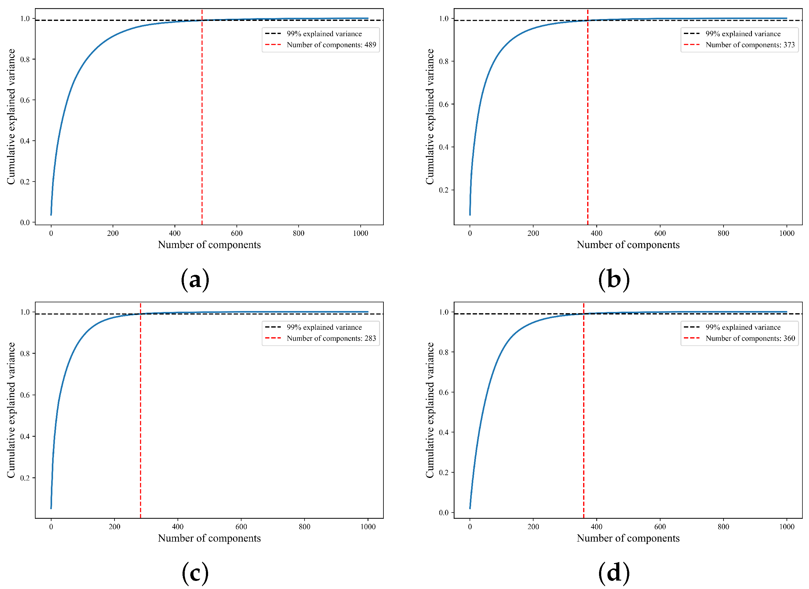
3.3. Adaptive Sample Length Selection

To address the issue of uneven sample lengths in the data collection process, this study sets four different equidistant samplings with specific lengths for different categories of bearing states as detailed in Table 1. In the context of 1D-CNN, consistent sample lengths are essential for model training. Thus, this paper introduces an adaptive sample length selection approach using the PCA algorithm on normalized bearing data of varying lengths. The selection process involves determining the number of principal components to retain based on the cumulative variance explained ratio, which signifies the proportion of variance explained by each component in the original data. A higher cumulative variance explained ratio indicates a better retention of fault information while reducing data dimensionality.
The number of principal components corresponding to a cumulative variance explained ratio [34] higher than 99% is chosen as the final dimensionality reduction in PCA. Specifically, in Figure 5a–d, respectively, the curves between the number of principal components and the variance contribution rate obtained by PCA analysis for four sample lengths are represented: 1024, 1004, 1014, and 1034. In Figure 5a–d, it can be observed that the numbers of principal components reaching an over 99% variance contribution rate initially are 489, 373, 283, and 360, respectively. This paper selects the maximum number of principal components as the final dimensionality reduction dimension for all samples.
After dimensionality reduction using PCA on the normalized bearing dataset, the sample length of all 10 bearing states becomes 489. The corresponding curve shape after dimensionality reduction is shown in Figure 6. By adaptively selecting sample lengths when they are uneven, it is possible to increase the model’s generalization ability and improve the training efficiency of the model in complex situations. Furthermore, this allows for the extraction and learning of key fault information, ultimately enhancing the diagnostic accuracy of the model.

3.4. Correlation Analysis of Data after PCA Dimensionality Reduction

In this section, we calculate the Pearson correlation coefficients [35] between the 10 bearing states to obtain similarity information, enabling an intuitive analysis of the correlation between the states after dimensionality reduction. The resulting Pearson correlation coefficient matrix is presented in Figure 7.
In Figure 7, we observe that the matrix is symmetric about the diagonal. The correlation coefficient values between categories labeled one and nine is 0.121, between categories labeled one and four is 0.113, and between categories labeled five and eight is 0.098. Positive values indicate relatively strong positive correlations between categories. On the other hand, the correlation coefficient between categories labeled one and six is −0.225, between categories labeled one and eight is −0.147, and between categories labeled seven and eight is −0.181. Negative values indicate relatively strong negative correlations between categories.
The Pearson correlation coefficient values closer to 1 (positive correlation) or −1 (negative correlation) indicate similarities in the data characteristics between the two categories, reflecting a stronger linear relationship and closer association between them. From the analysis, it is evident that Category 1 exhibits significant correlations with many other categories, implying that certain data features in Category 1 share similarities with data from other categories.

3.5. The Adaptive Sample Length-Adjusted 1DCNN-SeNet Diagnostic Model

The framework of the Adaptive Sample Length-Adjusted 1DCNN-SeNet Bearing Fault Diagnosis Model proposed in this paper is shown in Figure 8, which consists of three convolution–pooling layers, one SeNet layer, two fully connected layers, and one output layer. The specific algorithm model parameters are listed in Table 2.
In the algorithm model constructed in this paper, the PCA-adapted dimensionality-reduced bearing signals are used as the input to optimize the model’s performance and accelerate its convergence speed. In the model, the number of convolution kernels in the convolutional and pooling layers doubles layer by layer. Multiple one-dimensional convolutional kernels can learn features of different scales, while pooling operations reduce data dimensions and parameters. Multiple convolution–pooling combination layers gradually enlarge the receptive field, learning local features over broader ranges in the bearing signals, thereby extracting more advanced and abstract features. The SeNet layer has a feature compression ratio set to 16. It employs an attention mechanism, enabling adaptive learning of the importance of each channel and dynamically adjusting feature weights to enhance the model’s focus on key features, further exploring important fault features. Two fully connected layers process the feature output by the SeNet layer, helping the model capture complex correlations between various local features and perform feature combination and classification through weight matrices. The output layer is a Softmax layer, ultimately outputting a probability distribution vector for each category.
Throughout the entire experiment, the Windows 10 operating system was utilized, along with NVIDIA GeForce GTX1650 GDDR5 4g graphics card (Jijia Technology, Taipei, China). Python served as the primary programming language, with Pycharm 2023.3.2 as the compiling platform and Anaconda3 providing the base environment library. Data preprocessing was carried out using Numpy and Pandas libraries, while the PCA module from the SciPy library was employed for principal component analysis. For constructing the 1DCNN-SeNet model, Pytorch 1.10.2 along with Pytorch-cuda 12.1 for GPU acceleration were utilized. This framework offers a rich set of neural network components and training tools, facilitating the construction and training of complex neural network models. During training, the number of iterations was set to 100 epochs, with a batch size of 64 samples. The Adam optimizer was used for updating learning parameters, with a learning rate set to 0.001. Cross-entropy loss function was employed to measure the difference between the diagnostic model output and the true labels.

3.6. Analysis of Experimental Results

After PCA adaptive dimensionality reduction, the bearing dataset is randomly shuffled and split in a ratio of 6:2:2, resulting in a training set containing 6000 samples, a validation set containing 2000 samples, and a test set containing 2000 samples.

3.6.1. Model Training

In order to validate the effectiveness and superiority of the proposed model algorithm in this paper, we conducted comparative experiments with four classical algorithms: CNN [36], DNN [37], RNN [38], and ResNet18 [39]. We fed the 6000 samples from the training set into each model for feature learning. By observing the change curves of accuracy and loss values during training, as shown in Figure 9, it can be seen that around 50 iterations, the curves of accuracy and loss values tend to stabilize, indicating that the five models are basically in a convergent state at this point. This result helps to illustrate the performance of each model during training and provides important references for evaluating their performance.
In Figure 9a, it can be observed that the proposed 1DCNN-SeNet diagnostic method in this paper exhibits a faster convergence rate in the accuracy change curve and maintains a higher accuracy value after reaching a stable state. Compared to the other four comparative algorithms, this method shows the best performance in terms of accuracy. Meanwhile, the DNN algorithm shows significant fluctuations around approximately 43 iterations, while the convergence speed of the RNN algorithm is relatively slow compared to other algorithms. The ResNet18 algorithm exhibits slight fluctuations between 0 and 40 iterations, and the CNN algorithm performs well throughout the training process but still exhibits some minor fluctuations in the later stages. Overall, the proposed 1DCNN-SeNet diagnostic method demonstrates a significant advantage in terms of the accuracy change curve, while other algorithms exhibit varying degrees of fluctuations or slower convergence speeds.
According to Figure 9b, it can be observed that the proposed 1DCNN-SeNet diagnostic method in this paper exhibits the characteristic of having the lowest initial loss value in the loss change curve and maintains a stable low-value state throughout the entire iteration process compared to the other four comparative algorithms. This indicates that the method has a significant advantage in terms of loss value, demonstrating better convergence performance and stability compared to other algorithms.
During mini-batch training, we utilize the 2000 samples from the validation set as an additional dataset for model validation. In each iteration, a small batch of training samples is used to update the model parameters, and the validation set data are used within the same batch to compute metrics such as loss value and accuracy. If the model achieves the minimum loss value on the validation set, we save the model parameters from that iteration as the optimal solution. This approach allows for us to prevent overfitting by supervising the model with the validation set and ensures that the selected optimal model parameters possess good generalization capabilities. Additionally, comparing the optimal solutions obtained from different model iterations enables us to evaluate their performance on the specific task.

3.6.2. Model Testing

After loading the optimal solution parameters saved from the validation set into the model, we input the 2000 samples from the testing set into the five comparative algorithms for testing. This step aims to evaluate the performance of each model on unseen data and validate their generalization capability and practicality. The classification accuracies of different models are shown in Table 3.
According to Table 3, it can be observed that compared to the other four model algorithms, the 1DCNN-SeNet constructed in this paper achieved the highest accuracy in fault diagnosis, reaching 99.30% with a standard deviation of only 0.009. Having a higher accuracy and lower data fluctuation implies that the diagnostic model constructed in this paper can accurately identify fault categories with outstanding precision in fault diagnosis tasks, and the diagnostic results are more stable, ensuring accurate diagnosis under various conditions and reducing the error rate of fault classification. Compared to the CNN diagnostic model, the average accuracy of this paper’s diagnostic method increased by 0.25%, indicating that integrating the SeNet network model into the diagnostic method proposed in this paper contributes to improving the accuracy of the model. It has better feature extraction and representation capabilities, thereby enhancing performance in fault diagnosis tasks. The average accuracy of the method proposed in this paper is 99.3%, which is higher than the CNN in reference [40] by 0.41% and SE-ResNet152 in reference [41] by 2.88%. This improvement demonstrates the superior performance and effectiveness of the proposed method compared to the existing models cited in the references.
This paper introduces confusion matrices to evaluate the performance of the five fault diagnosis models, demonstrating the correspondence between predicted results and actual situations in each category. The confusion matrices of the five diagnostic models are shown in Figure 10. In these confusion matrices, each row represents the true category, each column represents the diagnostic category predicted by the model, and the numerical values in each cell indicate the number of samples that actually belong to the row category but are predicted as the column category. The intuitive display of confusion matrices allows for us to gain a clearer understanding of the performance of the diagnostic models in each category. By comparing the five confusion matrix graphs, it can be observed that the 1DCNN-SeNet fault diagnosis model constructed in this paper has the fewest misclassifications, demonstrating the superiority and effectiveness of the proposed method.

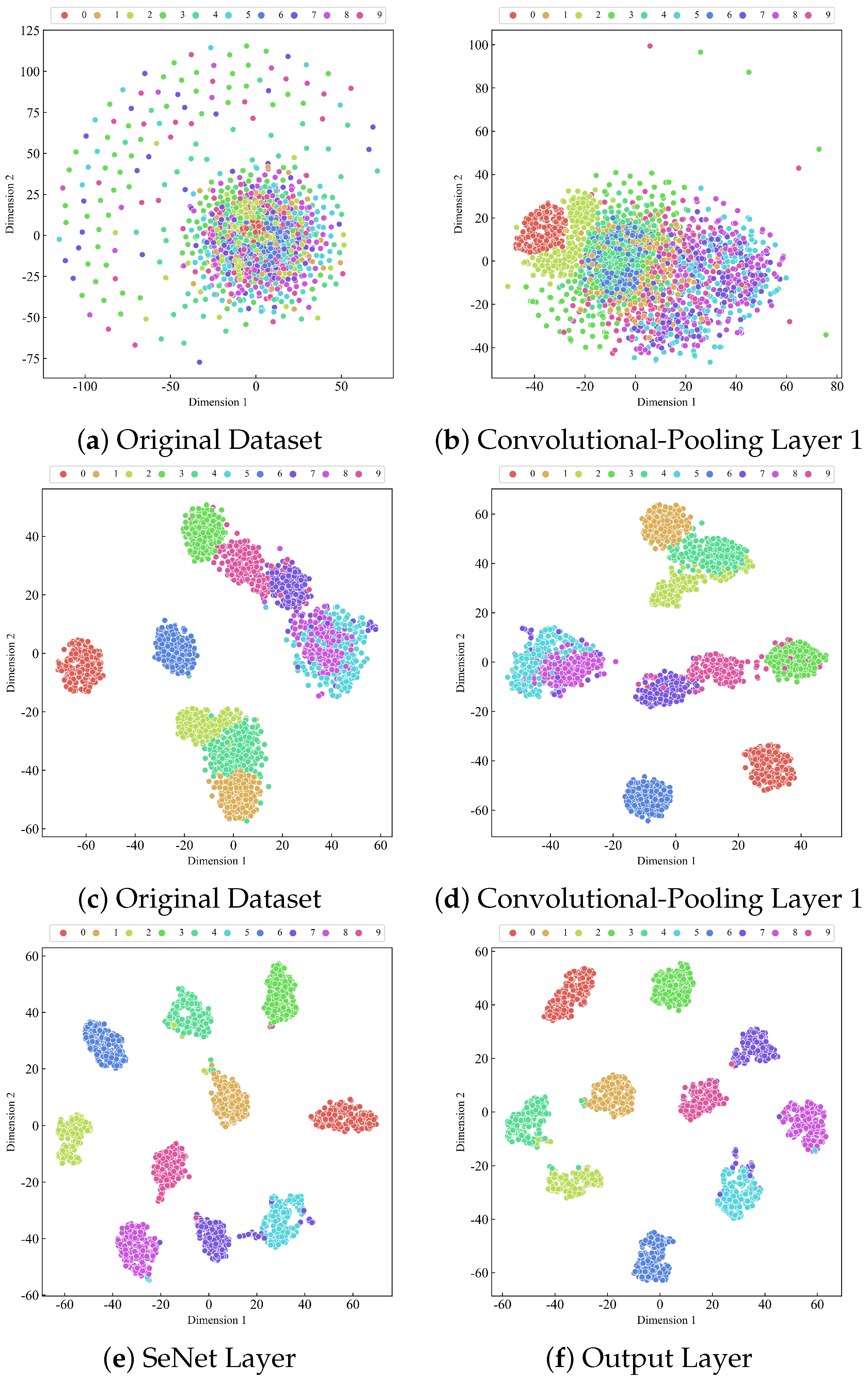
3.6.3. t-SNE Visualization Analysis

In order to gain a more comprehensive understanding of the features learned by the neural network at different network layers, this paper utilizes the t-SNE algorithm [42] to map high-dimensional features into a two-dimensional space and visualize them. The specific feature learning effect is shown in Figure 11. Through t-SNE visualization, we can directly observe the clustering and distribution patterns of different data categories in the feature space. This enables us to analyze and compare the features learned at different network layers, helping to assess whether the model effectively captures the key features of the data and aiding in understanding the model’s classification and generalization capabilities.
From Figure 11, it can be observed that the 10 categories of the original dataset are in a complex and intertwined state, making it difficult to distinguish each category. After the first convolution–pooling layer, samples from each category in the original dataset start to converge together and exhibit a certain degree of differentiation. After two convolution–pooling layers, samples corresponding to each category further cluster together, showing a clear distinction, but there are still some overlapping phenomena between categories. After the SeNet layer, the differentiation between the 10 categories is further enhanced, making them more clearly distinguishable. Finally, after the output layer, the 10 categories can be basically distinguished, forming distinct clusters in the feature space.
Through clustering analysis using the t-SNE algorithm, it is evident that the model constructed in this paper can effectively differentiate samples from different categories, demonstrating its outstanding performance in feature learning and classification tasks with high efficacy and accuracy. Furthermore, through t-SNE visualization, we are able to intuitively observe the distribution of data in the feature space, gaining insights into how the model understands and processes the data, thereby providing important references for further optimizing and improving the model. In conclusion, t-SNE clustering results reflect the excellent performance and generalization ability of the model, providing a solid foundation for its application and extension.

4. Summary

The paper introduces a fault diagnosis model, 1DCNN-SeNet, based on adaptive sample length adjustment designed to address the challenge of uneven sample lengths in bearing signal data collection or fault diagnosis. By conducting fault diagnosis on the CWRU bearing fault dataset, the effectiveness of the proposed method is validated, leading to the following conclusions:
(1)
This paper utilizes a PCA algorithm to adaptively adjust the uneven sample lengths, ensuring effective fault diagnosis on samples of different lengths based on the actual length of the input signal.
(2)
The 1DCNN network effectively captures the local temporal features of the bearing signal, while the SeNet network adaptsively learns the importance of features from each channel, automatically selecting and enhancing the features most helpful for bearing fault diagnosis. The combination of the two enables a more comprehensive capture of fault features in the bearing signal, thereby improving the accuracy and generalization capability of fault diagnosis.
(3)
Comparative analysis with four classical fault diagnosis algorithms demonstrates the significant advantages of the proposed model in bearing fault diagnosis tasks. It exhibits better adaptability to complex fault scenarios and different datasets, thus proving the effectiveness and superiority of the proposed algorithm.
(4)
Based on the research conducted in this paper, future endeavors could involve expanding the dataset to include a wider range of fault types and larger-scale real bearing fault data. This expansion would facilitate more comprehensive fault diagnosis and allow for deeper performance evaluation and comparative analysis of model algorithms. Additionally, it would be beneficial to seek engineering practical cases and apply the established models in real-world scenarios to validate their effectiveness.

Author Contributions

Methodology, F.X. and Z.S.; Validation, J.X.; Formal analysis, Z.S.; Resources, J.Y. and J.X.; Data curation, J.Y.; Writing—original draft, F.X.; Writing—review & editing, Z.S.; Funding acquisition, F.X. All authors have read and agreed to the published version of the manuscript.

Funding

Quzhou City Science and Technology Plan project (2023K263, 2023K265, 2023K045); General Research Project of Zhejiang Provincial Department of Education (2023) (Y202353440, Y202353289); Key project of Quzhou College of Technology (QZYZ2305).

Data Availability Statement

The data presented in this study are available in the article.

Conflicts of Interest

The authors declare no conflict of interest.

References

  1. Pattnayak, M.R.; Ganai, P.; Pandey, R.K.; Dutt, J.K.; Fillon, M. An overview and assessment on aerodynamic journal bearings with important findings and scope for explorations. Tribol. Int. 2022, 174, 107778. [Google Scholar] [CrossRef]
  2. Peng, B.; Bi, Y.; Xue, B.; Zhang, M.; Wan, S. A Survey on Fault Diagnosis of Rolling Bearings. Algorithms 2022, 15, 347. [Google Scholar] [CrossRef]
  3. Zhang, D.; Chen, Y.; Guo, F.; Karimi, H.R.; Dong, H.; Xuan, Q. A New Interpretable Learning Method for Fault Diagnosis of Rolling Bearings. IEEE Trans. Instrum. Meas. 2020, 70, 1–10. [Google Scholar] [CrossRef]
  4. Mikić, D.; Desnica, E.; Kiss, I.; Mikić, V. Reliability Analysis of Rolling Ball Bearings Considering the Bearing Radial Clearance and Operating Temperature. Adv. Eng. Lett. 2022, 1, 16–22. [Google Scholar] [CrossRef]
  5. Kim, T.; Han, J. Comparison of the Dynamic Behavior and Lubrication Characteristics of a Reciprocating Compressor Crankshaft in Both Finite and Short Bearing Models©. Tribol. Trans. 2004, 47, 61–69. [Google Scholar] [CrossRef]
  6. Vasić, M.; Stojanović, B.; Blagojević, M. Fault Analysis of Gearboxes in Open Pit Mine. Appl. Eng. Lett. 2020, 5, 50–61. [Google Scholar] [CrossRef]
  7. Xu, Z.; Chen, X.; Li, Y.; Xu, J. Hybrid Multimodal Feature Fusion with Multi-Sensor for Bearing Fault Diagnosis. Sensors 2024, 24, 1792. [Google Scholar] [CrossRef]
  8. Feng, A.; Xu, G.; Chen, C.; Liu, B.; Wei, Y.; Pan, X. Surface characteristics and wear resistance of GCr15 bearing steel by cryogenic treatment-laser peening. Appl. Phys. 2022, 128, 921. [Google Scholar] [CrossRef]
  9. Ashwini, K.; Rudraswamy, S.B. Automated inspection system for automobile bearing seals. Mater. Today Proc. 2020, 46, 4709–4715. [Google Scholar] [CrossRef]
  10. Baart, P.; Lugt, P.M.; Prakash, B. On the Normal Stress Effect in Grease-Lubricated Bearing Seals. Tribol. Trans. 2020, 57, 939–943. [Google Scholar] [CrossRef]
  11. Wang, D.; Tsui, K.; Qin, Y. Optimization of segmentation fragments in empirical wavelet transform and its applications to extracting industrial bearing fault features. Measurement 2019, 133, 328–340. [Google Scholar] [CrossRef]
  12. Sun, W.; An Yang, G.; Chen, Q.; Palazoglu, A.; Feng, K. Fault diagnosis of rolling bearing based on wavelet transform and envelope spectrum correlation. J. Vib. Control 2013, 19, 924–941. [Google Scholar] [CrossRef]
  13. Zhang, H.; He, Q. Tacholess bearing fault detection based on adaptive impulse extraction in the time domain under fluctuant speed. Meas. Sci. Technol. 2020, 31, 074004. [Google Scholar] [CrossRef]
  14. Li, G.; Wen, C.; Huang, G.; Chen, Y. Error tolerance based support vector machine for regression. Neurocomputing 2011, 74, 771–782. [Google Scholar] [CrossRef]
  15. Rostami, S.; Toghraie, D.; Shabani, B.; Sina, N.; Barnoon, P. Measurement of the thermal conductivity of MWCNT-CuO/water hybrid nanofluid using artificial neural networks (ANNs). J. Therm. Anal. Calorim. 2020, 2, 1097–1105. [Google Scholar] [CrossRef]
  16. Song, X.; Wei, W.; Zhou, J.; Ji, G.; Hussain, G.; Xiao, M.; Geng, G.S. Bayesian-Optimized Hybrid Kernel SVM for Rolling Bearing Fault Diagnosis. Sensors 2023, 23, 5137. [Google Scholar] [CrossRef] [PubMed]
  17. Yanting, A.; Jiaoyue, G.; Fei, C.; Jing, T.; Fengling, Z. Fusion information entropy method of rolling bearing fault diagnosis based on n-dimensional characteristic parameter distance. Mech. Syst. Signal Process. 2017, 88, 123–136. [Google Scholar]
  18. Saxena, A.; Saad, A. Evolving an artificial neural network classifier for condition monitoring of rotating mechanical systems. Appl. Soft Comput. 2007, 7, 441–454. [Google Scholar] [CrossRef]
  19. Liu, X.; Bo, L.; Luo, H. Bearing faults diagnostics based on hybrid LS-SVM and EMD method. Measurement 2015, 59, 145–166. [Google Scholar] [CrossRef]
  20. Zhao, M.; Lin, J.; Xu, X.; Li, X. Multi-Fault Detection of Rolling Element Bearings under Harsh Working Condition Using IMF-Based Adaptive Envelope Order Analysis. Sensors 2014, 14, 20320–20346. [Google Scholar] [CrossRef]
  21. Zhu, J.; Hu, T.; Jiang, B.; Yang, X. Intelligent bearing fault diagnosis using PCA–DBN framework. Neural Comput. Appl. 2019, 32, 10773–10781. [Google Scholar] [CrossRef]
  22. Lei, C.; Xia, B.; Xue, L.; Jiao, M. Zhang Huqiang.Rolling bearing fault diagnosis method based on MTF-CNN. J. Vib. Shock 2022, 9, 41. [Google Scholar]
  23. Dong, S.; Li, Y.; Liang, T.; Zhao, X.; Hu, X.; Pei, X.; Zhu, P. Fault Diagnosis Method of Rolling Bearing Based on CNN-BiLSTM Under Variable Working Conditions. J. Vib. Meas. Diagn. 2022, 42, 1009–1016+1040. [Google Scholar] [CrossRef]
  24. Li, K.; He, S.; Su, L.; Gu, J.; Su, W.; Lu, L. Full Vector Autogram Based Fault Diagnosis Method for Rolling Bearing. J. Vib. Meas. Diagn. 2023, 43, 298–303+410. [Google Scholar] [CrossRef]
  25. Lu, F.; Tong, Q.; Feng, Z.; Wan, Q.; An, G.; Li, Y.; Wang, M.; Cao, J.; Guo, T. Explainable 1DCNN with demodulated frequency features method for fault diagnosis of rolling bearing under time-varying speed conditions. Meas. Sci. Technol. 2022, 33, 095022. [Google Scholar] [CrossRef]
  26. Uddin, M.P.; Mamun, M.A.; Afjal, M.I.; Hossain, M.A. Information-theoretic feature selection with segmentation-based folded principal component analysis (PCA) for hyperspectral image classification. Int. J. Remote Sens. 2021, 42, 286–321. [Google Scholar] [CrossRef]
  27. Wang, T.; Xu, H.; Han, J.; Elbouchikhi, E.; Benbouzid, M.E.H. Cascaded H-Bridge Multilevel Inverter System Fault Diagnosis Using a PCA and Multiclass Relevance Vector Machine Approach. IEEE Trans. Power Electron. 2015, 30, 7006–7018. [Google Scholar] [CrossRef]
  28. Jia, G.W.; Zhang, X.; Wang, X.; Zhang, X.; Huang, N. A spindle thermal error modeling based on 1DCNN-GRU-Attention architecture under controlled ambient temperature and active cooling. Int. J. Adv. Manuf. Technol. 2023, 127, 1525–1539. [Google Scholar] [CrossRef]
  29. Li, B.; Lu, Z.; Jin, X.; Zhao, L. Tool wear prediction in milling CFRP with different fiber orientations based on multi-channel 1DCNN-LSTM. J. Intell. Manuf. 2023, 1–20. [Google Scholar] [CrossRef]
  30. Huang, J.; Ren, L.; Zhou, X.; Yan, K. An Improved Neural Network Based on SENet for Sleep Stage Classification. IEEE J. Biomed. Health Inform. 2022, 26, 4948–4956. [Google Scholar] [CrossRef]
  31. Xu, Y.; Jiang, X. Short-term power load forecasting based on BiGRU-Attention-SENet model. Energy Sources Part Recover. Util. Environ. Eff. 2022, 44, 973–985. [Google Scholar] [CrossRef]
  32. Aditya, A.; Zhou, L.; Vachhani, H.; Chandrasekaran, D.; Mago, V.K. Collision Detection: An Improved Deep Learning Approach Using SENet and ResNext. In Proceedings of the 2021 IEEE International Conference on Systems, Man, and Cybernetics (SMC), Virtual, 17–20 October 2021; pp. 2075–2082. [Google Scholar]
  33. Yoo, Y.; Jo, H.; Ban, S. Lite and Efficient Deep Learning Model for Bearing Fault Diagnosis Using the CWRU Dataset. Sensors 2023, 23, 3157. [Google Scholar] [CrossRef] [PubMed]
  34. Li, Q.; Tan, W.; Zhao, L.; Luo, H.; Zhou, Z.; Zhang, Y.; Bi, R.; Zhao, L. A Comprehensive Evaluation of 45 Pomegranate (Punica Granatum L.) Cultivars Based on Principal Component Analysis and Cluster Analysis. Int. J. Fruit Sci. 2023, 23, 135–150. [Google Scholar] [CrossRef]
  35. Li, G.; Zhang, A.; Zhang, Q.; Wu, D.; Zhan, C. Pearson Correlation Coefficient-Based Performance Enhancement of Broad Learning System for Stock Price Prediction. IEEE Trans. Circuits Syst. II Express Briefs 2022, 69, 2413–2417. [Google Scholar] [CrossRef]
  36. Shin, H.; Roth, H.R.; Gao, M.; Lu, L.; Xu, Z.; Nogues, I.; Yao, J.; Mollura, D.J.; Summers, R.M. Deep Convolutional Neural Networks for Computer-Aided Detection: CNN Architectures, Dataset Characteristics and Transfer Learning. IEEE Trans. Med. Imaging 2016, 35, 1285–1298. [Google Scholar] [CrossRef]
  37. Taheri, M.; Ahmadilivani, M.H.; Jenihhin, M.; Daneshtalab, M.; Raik, J. APPRAISER: DNN Fault Resilience Analysis Employing Approximation Errors. In Proceedings of the 2023 26th International Symposium on Design and Diagnostics of Electronic Circuits and Systems (DDECS), Tallinn, Estonia, 3–5 May 2023; pp. 124–127. [Google Scholar]
  38. Borandag, E. Software Fault Prediction Using an RNN-Based Deep Learning Approach and Ensemble Machine Learning Techniques. Appl. Sci. 2023, 13, 1639. [Google Scholar] [CrossRef]
  39. Kang, Y.; Chen, G.; Pan, W.; Wei, X.; Wang, H.; He, Z. A dual-experience pool deep reinforcement learning method and its application in fault diagnosis of rolling bearing with unbalanced data. J. Mech. Sci. Technol. 2023, 37, 2715–2726. [Google Scholar] [CrossRef]
  40. Guo, J.; Wu, W.; Wang, C. A Novel Bearing Fault Diagnosis Method Based on the DLM-CNN Framework. In Proceedings of the 2023 38th Youth Academic Annual Conference of Chinese Association of Automation (YAC), Hefei, China, 27–29 August 2023; pp. 370–374. [Google Scholar]
  41. Wu, G.; Ji, X.; Yang, G.; Jia, Y.; Cao, C. Signal-to-Image: Rolling Bearing Fault Diagnosis Using ResNet Family Deep-Learning Models. Processes 2023, 11, 1527. [Google Scholar] [CrossRef]
  42. Feng, W.; Zhang, G.; Ouyang, Y.; Pi, X.; He, L.; Luo, J.; Yi, L.; Guo, Y. Fault Diagnosis of Oil-Immersed Transformer based on TSNE and IBASA-SVM. Recent Patents Mech. Eng. 2022, 15, 504–514. [Google Scholar]
Figure 1. Basic structure diagram of a one-dimensional convolutional neural network.
Processes 12 00702 g001
Figure 2. Basic structure diagram of the SENet network.
Processes 12 00702 g002
Figure 3. Experimental bearing equipment diagram.
Processes 12 00702 g003
Figure 4. Original waveform diagram of 10 bearing states.
Processes 12 00702 g004
Figure 5. Curve of number of principal components and corresponding variance contribution rate.
Processes 12 00702 g005
Figure 6. Waveform of 10 bearing states after PCA dimensionality reduction.
Processes 12 00702 g006
Figure 7. Pearson correlation coefficient matrix among the 10 bearing states.
Processes 12 00702 g007
Figure 8. Depiction of the framework of the adaptive sample length adjusted 1DCNN-SeNet model.
Processes 12 00702 g008
Figure 9. Change curves of accuracy and loss values during training for different models.
Processes 12 00702 g009
Figure 10. Confusion matrix of test results.
Processes 12 00702 g010aProcesses 12 00702 g010b
Figure 11. t-SNE visualization results of different network layers.
Processes 12 00702 g011
Table 1. Detailed information of the bearing dataset.
Data StatesData SymbolsFault Diameter/InchesNumber of Samples/UnitsSample LengthLabels
NormalNormal_1——100010240
Roller FaultB007_10.007100010241
Roller FaultB014_10.014100010242
Inner Race FaultIR007_10.007100010243
Inner Race FaultIR014_10.014100010244
Outer Race FaultOR007@6_10.007100010245
Outer Race FaultOR014@6_10.014100010246
Roller FaultB021_10.021100010047
Inner Race FaultIR021_10.021100010148
Outer Race FaultOR021@6_10.021100010349
In the data symbols, “Normal_1” represents normal bearing data for a 1HP motor load, while “OR007@6_1” represents faulty outer ring bearing data at the 6 o’clock position for a 1HP motor load. Other symbols follow a similar pattern.
Table 2. Detailed information of the bearing dataset.
Network LayerNumber of Convolutional Kernels and Number of NeuronsConvolutional Kernel SizeStepOutput Size
Convolutional layer 1321 × 31 × 132 × 489
Pooling layer 1321 × 21 × 232 × 244
Convolutional layer 2641 × 31 × 164 × 244
Pooling layer 2641 × 21 × 264 × 122
Convolutional layer 31281 × 31 × 1128 ×122
Pooling layer 31281 × 21 × 2128 × 61
SeNet layer---128 × 61
Fully connected layer11000--1000 × 1
Fully connected layer 2100--100 ×1
Output layer10--10 × 1
Table 3. Detailed information of the bearing dataset.
MethodAverage Accuracy %Standard Deviation
CNN99.050.015
DNN98.950.12
RNN97.650.26
ResNet1897.400.135
1DCNN-SeNet99.300.009
Disclaimer/Publisher’s Note: The statements, opinions and data contained in all publications are solely those of the individual author(s) and contributor(s) and not of MDPI and/or the editor(s). MDPI and/or the editor(s) disclaim responsibility for any injury to people or property resulting from any ideas, methods, instructions or products referred to in the content.

