Abstract
Hydrodynamic cavitation (HC) has a wide range of application scenarios. However, there are few studies on the HC treatment of food waste (FW). A Venturi device is designed and operated and plays a clear role in changing the characteristics of FW. The medium viscosity is often neglected when studying cavitation behavior by numerical simulations. We use the Herschel–Bulkley model to describe the viscosity curves of artificial FW samples obtained experimentally. RANS numerical simulation is carried out with a simplified 2D axisymmetric CFD-based model considering the non-Newtonian fluid properties. A numerical simulation study is carried out for FW (TS = 10.0 wt%) at pressure drop ( = 0.05–0.4 MPa). The numerical simulation results show the variation of flow characteristics, viscosity, vapor volume, turbulent viscosity ratio, cavitation number, and pressure loss coefficient. With the increase in , the flow rate in the Venturi throat increases, and the average viscosity decreases. It reduces the inhibition effect of viscosity on cavitation. The position of incipient vacuoles at the moment of cavitation is constant and unrelated to the variation of . Under the effect of increasing , the average vapor volume fraction is increased, and the cavitation effect is enhanced; the cavitation number () is decreased, and the cavitation potential is improved. A larger should be selected to increase the cavitation efficiency of the device.
1. Introduction
With the development of the global economy and the rising consumption level of life, food waste (FW) treatment has become a global problem. It severely challenges the environment, economy, and society [1,2]. Achieving sustainability in FW treatment is essential to promote public health, resource availability, and ecological benefits. FW is collected from homes, restaurants, dining halls, and farm produce markets [3,4]. It is essential to reduce FW generation at source and to collect, treat, and recycle it. Food waste, including carbohydrates, lipids, and protein [5,6], can be transformed into bioethanol, biodiesel, and bio-oil [7], as well as high-value animal protein and premium organic fertilizers [8], enhancing resource utilization. However, the content of FW as well as its physicochemical and biological features have a significant impact on the overall process, particularly in terms of product yield and degradation rate [9]. To overcome these challenges, various types of pretreatments are possible, such as mechanical [10], thermal [11], alkaline/acid [12], enzymatic methods [13], etc., under four main categories, which are physical, chemical, biological, and combined. They are aimed at crushing, separation of oil–water–solid, and partial degradation, creating a positive environment for the subsequent treatment of food waste.
Cavitation is an important and complex flow with high 3D properties and high instability, and it has long been one of the most demanding critical problems in fluid mechanics. It has been widely applied for disinfection [14,15], cell disruption [16], sludge treatment [17], bio-diesel synthesis [18], nano-emulsion production [19], polymer degradation [20], and degradation of various organic compounds such as pharmaceutical drug residues [21], pesticides, textile dyes, and phenolics [22]. It can be categorized into four distinct groups, delineated by the manner of generation: optical cavitation, particle cavitation, acoustic cavitation, and hydrodynamic cavitation (HC) [16]. Hydrodynamic cavitation is the bubble generation and bursting process in a fluid due to local pressure changes. During the HC process, a significant amount of energy has the potential to be released into the surrounding liquid medium, resulting in thermal, mechanical, and chemical effects [15]. HC represents a technology with considerable potential for process intensification. It offers notable advantages such as enhanced energy efficiency, cost-effective operation, the ability to facilitate chemical reactions, and scalability. Importantly, HC achieves these benefits without requiring high-temperature and -pressure conditions. Combined with other pretreatment methods, it achieves enhanced effects and energy savings [23]. The application fields of HC are numerous and extensive, and the following will only take sludge treatment in the environment as an example. During cavitation, mechanical shear stress [24], temperature [25], and oxidizing effects of free radicals [26] can result in the breakdown of sludge aggregates and the subsequent liberation of both intracellular and extracellular substances. Using it reduced the average particle size [25], enhanced dewatering [17,27], and increased the biological treatment potential of sludge [28]. However, research on using HC for FW treatment has not yet been reported.
Cavitation numerical simulation is an important auxiliary for cavitation research [29]. In the early 1990s, with the development of computer technology, cavitation models were proposed to describe the cavitation phenomenon using computational fluid dynamics (CFD) methods [30]. It can reduce the time and energy consumed in experimental studies and reveals more flow field details than in experimental studies [31]. It can be associated with some experimental optimization methods, such as response surface methodology (RSM) [31,32], proper orthogonal decomposition (POD) [33], etc., to optimize different HC processes. With cavitation flow, as a typical multiphase flow problem, when using CFD for HC numerical simulations, cavitation models, turbulence closures, and multiphase modeling approaches are needed [34]. Therefore, selecting a reliable method for modeling cavitation should be essential. The viscosity of the cavitation medium is a necessary parameter when using cavitation simulations to analyze practical problems. When studying HC occurring in media with water as the main component, the viscosity of water is used for cavitation simulations [31,32,35]. In the study of cavitation occurring in media with viscosity, a fixed viscosity parameter is mostly used, and the change in viscosity during cavitation is not considered [36,37,38]. In practice, the viscosity of the medium treated by HC is often more significant than that of water and maybe a non-Newtonian fluid whose viscosity changes with shear rates, such as that of the remaining activated sludge. The results are inaccurate, ignoring the viscosity and viscosity change of the cavitation medium and conducting numerical research on the cavitation device.
Based on the above review of the existing literature, we carried out an experimental and numerical study on the HC phenomenon of FW pretreatment. Due to food waste having typical non-Newtonian fluid characteristics, media viscosity and its variation are considered during the simulation and data validation. A two-phase flow (liquid–vapor) RANS CFD model is established and applied to describe the cavitation behavior at different Venturi pressure drops ().
2. Hydrodynamic Cavitation Pretreatment Test of Food Waste
2.1. Hydrodynamic Cavitation Device
An HC device (Figure 1) is designed and assembled to test the HC effect of FW pretreatment.
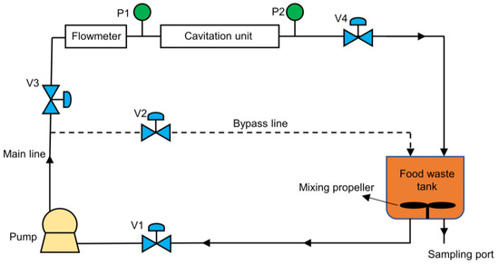
Figure 1.
Schematic diagram of HC device.
The device includes a Venturi (cavitation unit), pressure sensors arranged in the inlet and outlet of the Venturi, an electromagnetic flow meter, an FW tank, a 3.0 kW pressured pump, and four control valves, including V1, V2, V3, and V4. The lower portion of the tank is linked to the suction inlet of the pump, and the flow is then propelled into two separate conduits. The bypass flow can be used to adjust the pressure and flow of the medium in the device. To prevent any air induction, the main line and the bypass line are terminated within the tank at a position below the level of the solution. Four manual valves are placed at strategic locations to control the flow of the lines. The gauge pressure at inlet () is read by pressure sensor P1. The outlet gauge pressure () is read by pressure sensor P2. The Venturi pressure drop () is the difference between and . The flow is measured and recorded by an electromagnetic flow meter installed upstream of the pressure transducer. The device includes a water bath to keep the temperature stable. The cavitation unit is drawn in CAD and made using SLA-3D printing technology (Figure 2). The details of the cavitation unit are shown in Table 1.
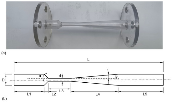
Figure 2.
Cavitation unit details. (a) Venturi photo. (b) Venturi sizes.

Table 1.
Details of the cavitation unit.
2.2. Composition of Food Waste
FW comes from a variety of sources, such as household waste, fruits and vegetables, and restaurant waste [39]. Many factors influence FW characteristics, including topography, seasonal variations, sources of collection, cooking methods, and patterns of consumption [40]. FW contains a complex material composition, including carbohydrates, cellulose, proteins, lipids, and salt [41]. FW is perishable and difficult to store. Therefore, the experiment uses artificial FW samples (Figure 3). Solid samples undergo lyophilization using a vacuum freezing drier and are subsequently sieved using a 60-mesh screen. The samples are promptly placed in a freezer for further examination. The composition of the FW sample is shown in Table 2. Solid samples are uniformly mixed with edible salt and soybean oil, and then diluted with deionized water. In subsequent experiments, they are used with different total solid concentrations (TS = 25.0 wt%, 20.0 wt%, 15.0 wt%, 10.0 wt%, 5.0 wt%, and 2.5 wt%).
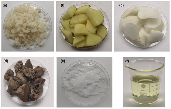
Figure 3.
The food waste samples. (a) Cooked rice. (b) Cooked potatoes. (c) Cooked radishes. (d) Cooked chicken livers. (e) Edible salt. (f) Soybean oil.
Table 2.
The composition of food waste.
2.3. Test Result
First, 500 mL of FW (TS = 25.0 wt%) is processed in the HC device for 10 min. Then, 15 mL of the sample is placed in a centrifuge tube and centrifuged at 5000 r/min for 10 min. The results are shown in Figure 4.
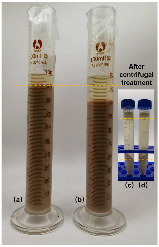
Figure 4.
Treatment effect of FW. (a) HC. (b) Without HC. (c) Centrifugation (after HC). (d) Centrifugation (without HC).
The sample in the centrifuge tube is divided into three layers: oil, water, and solid from top to bottom, and the interfaces are clear. After cavitation treatment, the volume of the upper oil layer is increased significantly, the water in the middle layer is clear and transparent, and the volume of the lower solid phase is decreased and becomes more compact. In the biological treatment of FW, oil has an apparent inhibitory effect on microbial reaction [42]. In general, the grease in FW is bonded with other components, making it difficult to remove oil directly. The oil floating on the upper layer of the centrifuge tube is called floating oil, which is convenient to collect and remove. HC pretreatment significantly increased the proportion of floating oil. Meanwhile, after cavitation treatment, the liquid phase of FW increased, and the solid phase decreased. This indicates that HC pretreatment promotes the decline of solid matter in FW.
3. Problem Formulation and Governing Equations
Cavitation refers to the phenomenon wherein the flow contracts because of the downstream pressure in the Venturi being lower than the vapor pressure of the liquid. When cavitation begins, flow fields become extremely turbulent, creating vapor cavities that finally collapse. It is difficult to numerically model such complex flow fields. Direct numerical simulation (DNS) is the best strategy for resolving events across such a wide range of time and length scales. However, this method of calculation incurs significant computing expenses. This study primarily investigates the impact of pressure on the FW cavitation in the Venturi. Therefore, the Reynolds averaged Navier–Stokes (RANS) methodology is utilized in this context. The -, turbulence model is utilized due to its distinct benefits in accurately forecasting flow separation and characterizing flow behavior in adverse pressure gradients. Additionally, it is the most widely used turbulence model for large-aspect-ratio industrial flow [43]. A mixing model is used to study FW cavitation in the Venturi. Considering the flow field in the Venturi is axisymmetric, and the modeling of the Venturi is carried out in a 2D computational domain. The computational grid is shown in Figure 5.
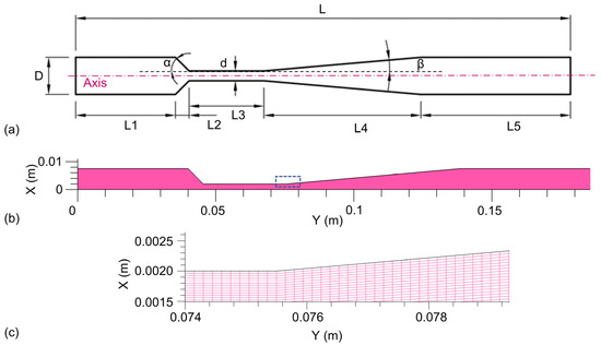
Figure 5.
Structured grid graph for computing (grid-2). (a) Cavitation unit size. (b) Full view. (c) Zoom view.
3.1. Flow and Turbulence Model
The following are the continuity and momentum equations for the mixture model:
Continuity equation [44]:
where
Momentum equation [44]:
The velocity of the mixed phase is denoted as , while the velocity of the individual phase is represented by . The symbol represents the density of the mixed phase. The symbols and represent the turbulent viscosity and the mixture phase viscosity, respectively. The expression for the turbulent viscosity in the SST k−ω, RANS model is given by the following equation [44]:
where is an input parameter that depends on the Reynolds number. and are the turbulent kinetic energy and the specific dissipation rate and defined by the following transport equations:
where
The variables , , , and represent the processes of creation and dissipation of turbulent kinetic energy () and specific dissipation rate () in the context of turbulence.
3.2. Cavitation Model
The Singhal model [45], the Schnerr–Sauer model [46], and the Zwart model [47] are widely recognized as the three most prominent cavitation models. The Singhal model is often referred to as a comprehensive cavitation model because of its inclusion of several factors such as the formation and movement of vapor bubbles, fluctuations in pressure and velocity, and the influence of non-condensable dissolved gases. The use of the Zwart cavitation model necessitates the inclusion of additional empirical calibration coefficients. These coefficients encompass parameters such as the constant bubble diameter, nucleation site volume fraction, evaporation coefficient, and condensation coefficient. The only parameter that requires determination in the Schnerr–Sauer cavitation model is the bubble number density. For simplicity, we use the Schnerr–Sauer cavitation model. Dutta et al. used the Schnerr–Sauer cavitation model in their study on Venturi cavitation using water as a medium [48]. Shi et al. used the same Schnerr–Sauer cavitation model in the study of cavitation [49].
The computation of the average vapor volume fraction in the Schnerr–Sauer model involves solving a transport equation for the vapor percentage [44]:
The symbol represents the volume percentage of the vapor phase. The symbol represents the density of the vapor phase. In contrast, and represent the mass transfer processes associated with evaporation and condensation during cavitation, respectively.
The mathematical representation for the values of and is expressed as follows [44]:
When
when
The variable represents the downstream pressure at full recovery. The formula for expressing the radius of a bubble is as follows [44]:
The expression for the volume fraction of the vapor is provided by [44]:
The bubble number density, denoted as , is utilized in this simulation with a value of 1013. Numerous scholarly sources indicate that the ideal value is 1013. Li et al. [50], Shi et al. [35], and Liu et al. [51] used the value of 1013 and obtained the correct results. The estimation of the saturation pressure, denoted as , is determined using the Antoine equation, which is expressed as follows [44]:
The material-specific constants are denoted by , , and . The vapor pressure, denoted as , is set at a value of 2350 Pa over the whole range of conditions encompassed in this simulation.
3.3. Boundary Conditions
The model uses the boundary conditions as shown in Table 3.
Table 3.
Boundary conditions used in the model.
At the inlet and exit of the Venturi, the inlet pressure and outlet pressure boundary conditions are employed. The gauge pressure at the inlet, denoted as , is subjected to a range of values from 0.05–0.4 MPa, while the outlet gauge pressure, referred to as , is constant at 0.0 MPa. The wall is subject to a no-slip condition. The specified values for turbulent intensity and turbulent viscosity ratio are 10% and 10, respectively.
Table 4 displays the physical parameters used in the model. To obtain the viscosity parameters, we tested the viscosity of FW with different total solid.
Table 4.
Physical parameters used in the model.
3.3.1. Viscosity Test Method
The viscosity of FW is measured with an HBDV-2T rotational viscometer. The viscometer has six rotors. The water bath heating system is set to maintain a temperature of 20 ± 0.5 °C. Viscosity measurement of FW (TS = 2.5 wt%, 5.0 wt%, and 10.0 wt%) is carried out using rotor 3#. The stirring speed is set as 5 r/min, 7 r/min, 9 r/min, 11 r/min, 13 r/min, 15 r/min, 17 r/min, 19 r/min, 21 r/min. Then, viscosity measurement of FW (TS = 15.0 wt%, 20.0 wt%, and 25.0 wt%) is carried out using rotor 2#. The stirring speed is set as 0.5 r/min, 1 r/min, 2 r/min, 3 r/min, 4 r/min, 5 r/min, 6 r/min, 7 r/min, 8 r/min, 9 r/min. The readings are recorded after stabilization at each speed, and the experiment is repeated three times.
3.3.2. Viscosity Test Results
Considering the properties of non-Newtonian fluids, the Herschel–Bulkley model (Equation (17)) is used to fit the measured data of the viscosity of FW with different total solid concentrations. FW samples (TS = 2.5–25.0 wt%) are tested using a rotational viscometer at 20 °C. The results are shown in Figure 6 and Table 5. Cao et al. [52] used the Herschel–Bulkley model to describe the viscosity of a mixture of sludge, FW, etc. Caillet et al. [53] found that the Herschel–Bulkley model could accurately describe the viscosity of anaerobically digestible materials, such as residual sludge viscosity. Garakani et al. [54] used the Herschel–Bulkley model to describe the viscosity of highly viscous sludge.
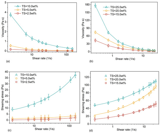
Figure 6.
Viscosity and shear stress curve of FW. (a) Viscosity curve (TS = 2.5 wt%, 5.0 wt%, and 10.0 wt%). (b) Viscosity curve (TS = 15.0 wt%, 20.0 wt%, and 25.0 wt%). (c) Shear stress curve (TS = 2.5 wt%, 5.0 wt%, and 10.0 wt%). (d) Shear stress curve (TS = 15.0 wt%, 20.0 wt%, and 25.0 wt%).
Table 5.
Parameters of food waste with different total solid.
The symbol represents the shear stress. The symbol represents yield stress. represents the consistency coefficient. represents the shear rate. represents the rheological consistency index.
When TS = 2.5 wt% and TS = 5.0 wt%, the shear stress curve is nearly straight, and the non-Newtonian characteristics of the fluid are weak. When TS ≥ 10.0 wt%, the shear stress and shear rate are non-linear. When the shear rate is low, the shear stress increases significantly. With increasing shear rate, the increase in shear stress leveled off. The FW exhibited shear-thinning rheological properties consistent with the characteristics of a pseudoplastic non-Newtonian fluid.
The larger the total solid of FW, the stronger its non-Newtonian fluid properties and the greater the viscosity after stabilization at high shear rates. The results are similar to those obtained by Baroutian et al. [55] for the viscosity of FW. From the microscopic point of view, the internal particle structure of FW is relatively loose. The increased shear rate destroys this loose particle structure and causes the particles to rearrange themselves. The destruction rate at the crosslinking point is greater than the reconstruction rate, which causes lower shear stress. When the total solid of FW is small, the distance between the solid particles of FW increases, the force between the particles decreases, and the viscosity decreases.
The above experiments measured the viscosity parameters of a non-Newtonian fluid of FW. To conveniently study the effect of on the hydraulic cavitation behavior of FW, the viscosity parameter of FW (TS = 10.0 wt%) is brought into the CFD model for the analysis.
3.4. Solution Methodology
The ANSYS Fluent (version 19.2) software is employed for the numerical solution of the governing differential equations and boundary conditions. This enables the visualization of the velocity field and volume fraction field within the flow domain. ICEM is used to draw the model and generate structured grids. The SIMPLE algorithm is utilized for pressure velocity coupling, and the PRESTO discrete format is used for pressure discretization.
The selection of the spatial discretization method for the volume fraction is carried out by the quadratic upwind interpolation for convection kinematics (QUICK) scheme. The momentum equation is discretized using the second-order upwind method. The discretization of time in the RANS model involves the utilization of the first-order implicit scheme.
To mitigate numerical oscillation in the solution, a relatively short time step = 1 × 10⁻⁵ s is employed. All numerical simulations exhibit time-dependent characteristics. Each simulation is performed with a total flow duration of 0.6 s. The temporal evolution of variables such as the mean vapor volume fraction and throat velocity is observed. They are stable after a flow time of 0.6 s. The convergence criterion for the continuity and momentum equations in this simulation is set at a value of 10−6. A grid independence test is performed to avoid the influence of numerical methods on experimental results. In addition, a comparative analysis is conducted between the numerical findings and the experimental data to find out about the dependability and precision of the research.
3.5. Mesh Sensitivity Analysis
In this section, before investigating the impact of geometric parameters on cavitating flow, the examination of grid resolution is conducted to establish an optimal grid size for the simulations. The study was conducted at = 0.1 MPa, utilizing three sets of grids consisting of 21,540 cells (Grid-1), 67,350 cells (Grid-2), and 269,400 cells (Grid-3). Simulations are conducted using same configurations for all three grids. The mesh statistics are shown in Table 6.
Table 6.
Mesh information.
The values of turbulent kinetic energy at the characteristic positions in the Venturi are shown in Figure 7.
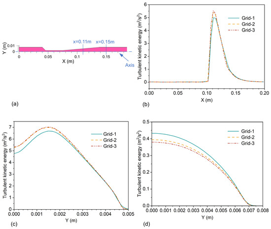
Figure 7.
The value of turbulent kinetic energy. (a) Position of the value. (b) At the axis. (c) x = 0.11 m. (d) x = 0.15 m.
The turbulent kinetic energies at the axis, at the radial position of x = 0.11 m, and at the radial position of x = 0.15 m are compared. The discrepancy seen between Grid-2 and Grid-3 is found to be below 2%. In general, increasing the resolution of the grid has the potential to yield improved numerical results. However, using a more refined grid is impeded by the substantial computational expenses associated with CPU and memory resources. Based on the previous experimental findings, Grid-2 is used for the rest of the simulations. Grid-2 meets experimental needs and has a low computational cost.
3.6. Numerical Model Validation Experiments
To verify the numerical results, the Venturi is simulated under the conditions of FW TS = 10.0 wt% and = 0.025–0.15 MPa. The results are shown in Figure 8.
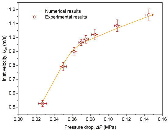
Figure 8.
Experimental and simulated as a function of inlet velocity.
The inlet velocity increases with the increase in , but the increment of the inlet velocity becomes smaller. This is because the cavitation phenomenon produces bubbles in the throat of the Venturi, and the bubbles slow down the increase in . Shi et al. [56] also observe similar phenomena in experimental verification. The results of the simulation show a high level of concordance with the empirical data, and the percentage error between experimental and numerical results is 4.6–9.2%.
This deviation is not rare. Simpson et al. [57] and Nagarajan et al. [58] also mentioned similar deviations. One possible explanation for this phenomenon could be the presence of dissolved non-condensable gases or suspended particulates within the fluid, which can have an impact on the extent of cavitation occurring in the Venturi. In addition, the physical and chemical effects of HC can dilute the FW to a certain extent. This can result in larger experimental values than simulated values of inlet velocity after the increasing of .
4. Results and Discussion
4.1. Flow Characteristics
The fluid flow characteristics within the Venturi can be utilized to anticipate the fluctuations in the average vapor volume fraction within the Venturi, helping with the prediction of the occurrence of cavitation. The magnitude of velocity and pressure in the Venturi are shown in Figure 9 and Figure 10.
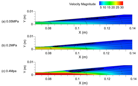
Figure 9.
Velocity magnitude contours at different .
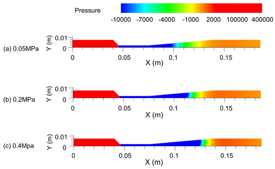
Figure 10.
Pressure contour lines at different .
The fluid pressure in the throat area decreases rapidly, the flow velocity increases, and the kinetic energy increases. As the pressure is further reduced to the saturated vapor pressure, the flow rate at the end of the throat reaches the maximum. The streamline in Figure 10 shows that the shape of the pipe in the divergent section changes the fluid flow direction in the pipe. The flow rate is faster near the X-axis and slower near the pipe wall. The fluid still maintains a fast flow rate in the divergent section. The vortex is formed in the diffusion section, and the increase in leads to the thickening of the vortex area and the decrease in the length, which is also the reason for the faster flow velocity near the X-axis. With the increase in the pressure difference , the distribution range of the high-speed region of the fluid in the Venturi increases, and the maximum velocity gradually increases. The range of the low-pressure area is also gradually increased, which provides favorable conditions for the growth and development of cavitation, which is conducive to enhancing the cavitation effect.
The variation of the maximum velocity in the Venturi is shown in Figure 11.
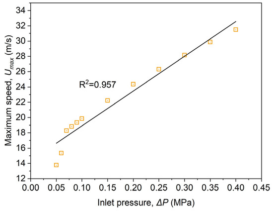
Figure 11.
The maximum velocity of Venturi throat variation with .
When the increases from 0.05 MPa to 0.4 MPa, the maximum velocity at the throat of the Venturi increases from 13.2 m/s to 32.7 m/s, and the maximum velocity is linearly positively correlated with . The throat is the characteristic section of the Venturi. The increase in the throat velocity indicates that the cavitation ability of the Venturi is enhanced. From the analysis of the flow characteristics in the Venturi, the increase in enhances the cavitation ability of the Venturi.
4.2. Viscosity
The viscosity of the medium in the Venturi will affect the cavitation intensity. High-viscosity medium will inhibit the generation of cavitation and reduce the cavitation intensity [59]. The variation of viscosity in the Venturi with various is shown in Figure 12.
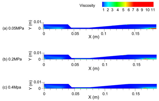
Figure 12.
Venturi viscosity contour.
The viscosity near the symmetry axis of the Venturi is higher than that of other parts. With the gradual increase in , the viscosity of the inlet portion of the Venturi gradually diminishes, while the viscosity of the Venturi throat grows, and the viscosity at the outlet of the Venturi drops. The average viscosity of the Venturi is extracted to evaluate the variation of the overall viscosity of the Venturi. The shear rate is directly related to the viscosity, so the average shear rate in the Venturi is also extracted.
The variation of average shear rate and average viscosity in the Venturi with various is shown in Figure 13.
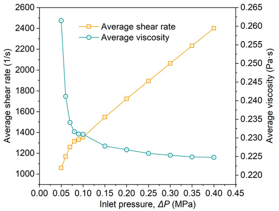
Figure 13.
Variation of average shear rate and average viscosity with in Venturi.
With the increase in , the average shear rate in the Venturi increases almost linearly. The average viscosity decreased rapidly and then decreased slowly. = 0.07 MPa is the turning point of the rate of viscosity decrease. The reason is that FW is a shear-thinning non-Newtonian fluid. The viscosity of FW will gradually decrease with the increase in shear rate and finally remain constant. In short, with the increase in , the flow velocity in the Venturi increases, and the turbulence increases. This phenomenon is caused by an increased average shear rate in the Venturi. The increase in increases the average shear rate in the Venturi. It reduces the average viscosity in the tube, which is beneficial to the improvement of cavitation intensity. From this study, when using the Venturi to pretreat FW (TS = 10.0 wt%), ≥ 0.07 MPa should be selected to ensure a significant reduction in viscosity.
4.3. Vapor Volume
Venturi average vapor volume fraction can determine the intensity of cavitation. The variation of average vapor volume fraction in the Venturi with various is shown in Figure 14.
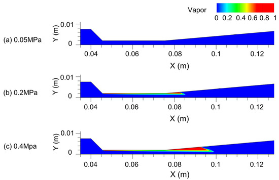
Figure 14.
Average vapor volume fraction at different . (a) = 0.05 MPa. (b) = 0.2 MPa. (c) = 0.4 MPa.
The cavitation bubbles are generated from the throat of the Venturi device and grow and develop in the diffusion section. Then, the bubbles collapse and dissipate in the high-pressure area downstream. As analyzed in Section 4.1, the flow in the throat region increases rapidly, and the pressure decreases to the saturated vapor pressure very quickly. The water in the FW vaporizes rapidly and generates vacuoles, which are named “incipient vacuoles.” The location where the first vacuoles are generated is called the incipient vacuole location.
The increasing provides a better bubble-growing environment. In the Venturi throat and diffusion section, the average vapor volume fraction is increased. The initial location of the cavitation bubbles is relatively fixed during the variation of .
The present study provides a quantitative assessment of the vapor fraction, specifically in terms of the average volume fraction. This measure is defined as follows:
The variation of the average vapor fraction in the Venturi with various is shown in Figure 15.
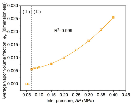
Figure 15.
Curve of average vapor volume fraction with .
The average vapor fraction () increases gradually with increasing , and the effect of increasing gas content is gradually accelerated. When < 0.07 MPa (Figure 15, region I), 0%, and HC does not occur in the Venturi. When = 0.07–0.4 MPa (Figure 15, region II), HC occurs, and the relationship between and can be expressed as:
The formula can calculate when using a Venturi to treat FW (TS = 10.0 wt%) in a pressure range of = 0.05–0.4 MPa.
The reason for this phenomenon is that the average viscosity in the Venturi decreases with increasing (Section 4.2). The decrease in viscosity promotes the increase in flow velocity. The high velocity of the flow allows the vapor bubbles in the diffusion section to grow and develop sufficiently, thus increasing the vapor content, which suggests that an increasing enhances the cavitation of the Venturi.
4.4. Turbulent Viscosity Ratio
The turbulent viscosity ratio, denoted as (), is defined as the ratio between the turbulent viscosity () and the molecular viscosity (). The estimation of turbulence inside the simulation domain requires the utilization of dynamic viscosities. The variation of turbulent viscosity ratio in the Venturi with various is shown in Figure 16.
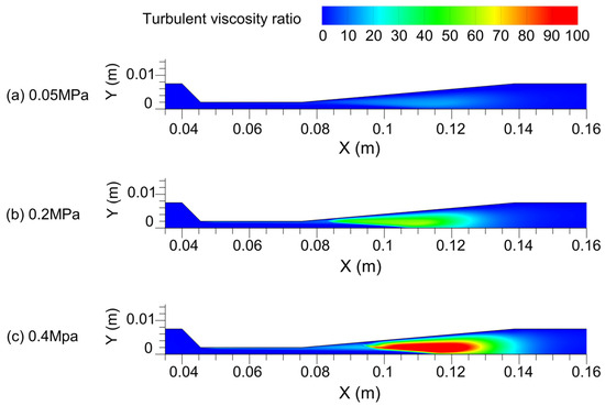
Figure 16.
Turbulent viscosity ratio at different inlet pressures. (a) = 0.05 MPa, (b) = 0.2 MPa, (c) = 0.4 MPa.
The observed data indicate that the maximum ratio of turbulence viscosity saw an increase from 14.6 to 120.7 as rose from 0.05 MPa to 0.4 MPa. For the Venturi at a certain pressure, the turbulent viscosity ratio of the dispersion section in the Venturi is higher. Turbulence occurs in the Venturi diffusion section (Figure 9). For the Venturi at different pressures, maximum turbulent viscosity increases with . This is because the viscosity of the medium in the Venturi decreases with increased (Section 4.2). The increased turbulent viscosity ratio leads to cavitation bubble collapse, which reduces cavitation gas production. Variation of the turbulent viscosity ratio in the diffusion section affects the location of cavitation bubble generation. The variation of vapor bubble generation position with is shown in Figure 14. In the diffusion section of the Venturi, the increase in turbulent viscosity ratio hinders the cavitation intensity.
4.5. Cavitation Number
The analysis of cavitation strength in the device involves the utilization of the cavitation number (), which is a specific dimensionless metric employed in the Venturi to assess the likelihood of cavitation occurrence. It is defined as the pressure drop between the throat and the downstream region of the cavitating device divided by the kinetic head at the throat. The cavitation number is defined as follows [60]:
where represents the fully recovered downstream pressure, represents the vapor pressure of the liquid at the reference temperature (), represents the density of the FW, and represents the flow velocity at the throat of the Venturi.
where represents the flow rate at the inlet, while denotes the diameter of the throat.
Cavitating flow occurs when , assuming ideal circumstances. However, when the cavitation number , cavitation may also occur. This is because the cavitation medium contains dissolved gas and particle impurities.
The variation of with is shown in Figure 17.
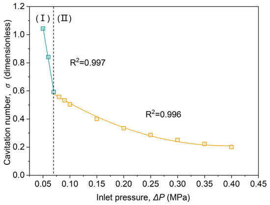
Figure 17.
The variation curve of cavitation number with pressure difference .
With the increase in , the cavitation number decreases gradually, and the trend of cavitation gradually increases. To obtain the cavitation number more conveniently, the curve is fitted. When = 0.05–0.07 MPa (Figure 17, region I), cavitation does not occur. can be shown as follows:
When = 0.07–0.4 MPa (Figure 17, region II), the cavitation occurs. can be expressed as:
The is calculated by fitting the formula. This obtains the cavitation number quickly and the cavitation capacity at the current can be evaluated.
4.6. Pressure Loss Coefficient
To investigate the pressure loss in Venturi cavitation systems at different , the dimensionless number is defined to represent the pressure loss in the Venturi. is defined as follows:
The symbol represents the difference in static pressure between the upstream and downstream pressures, while denotes the velocity at the inlet. The velocity at the inlet can be mathematically represented as:
The variation of the pressure loss coefficient () with is shown in Figure 18.
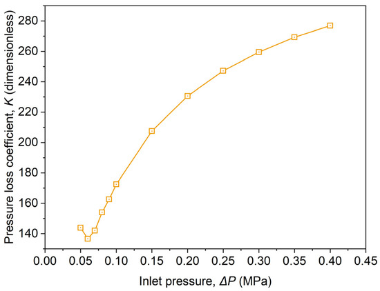
Figure 18.
Represents the effects of on pressure loss coefficient ().
The pressure loss coefficient decreases slightly and then increases monotonically with the increase in , and the rate of increase becomes slower with increasing . This is because the increasing leads to an increase in the cavitation intensity in the Venturi. Cavitation produces many bubbles in the diffusion section of the Venturi. These bubbles increase the resistance to fluid passage in the Venturi and increase the pressure loss.
In this paper, cavitation efficiency is defined to comprehensively evaluate the pressure loss coefficient and cavitation number of the Venturi.
where represents the cavitation number, which represents the ability of cavitation in the Venturi. The smaller the value, the stronger the cavitation ability. is the loss coefficient of pressure in the Venturi. The smaller the value, the smaller the loss of pressure.
The variation of cavitation efficiency () with is shown in Figure 19.
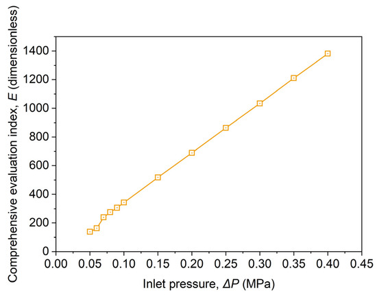
Figure 19.
The variation diagram of cavitation efficiency with .
The increases linearly with increasing in the range of 0.05–0.4 MPa. When using the Venturi to pretreat FW (TS = 10.0 wt%), a higher pressure should be used to ensure the highest cavitation efficiency.
5. Conclusions
We provide work on the experimental and numerical simulation of hydraulic cavitation pretreatment of food waste. The viscosity parameters of food waste (FW) are measured. Numerical simulations of the cavitation behavior are performed using a 2D CFD model, which considers the non-Newtonian fluid properties of the FW. Validation test results show that the predicted results are close to the experimental data. The effect of Venturi pressure drop ( on flow characteristics, viscosity, vapor volume, turbulent viscosity ratio, cavitation number, and pressure loss coefficient is studied numerically.
(1) The effect of oil–liquid–solid stratification is noticeable after food waste is pretreated by hydrodynamic cavitation (Venturi). HC pretreatment is beneficial for the separation of floating oil and can promote the decline of solid matter.
(2) Food waste is a shear-thinning non-Newtonian fluid, and the greater the total solid, the stronger the non-Newtonian characteristics.
(3) Food waste (TS = 10.0 wt%) is pretreated by a Venturi with = 0.05–0.4 MPa. The average viscosity in the Venturi decreased with the increase in , and the inhibition effect of viscosity on cavitation is reduced.
(4) For Venturi pretreatment of food waste (TS = 10.0 wt%), ≥ 0.7 MPa is necessary to ensure the cavitation occurs. With increasing , the position of incipient vacuoles in the Venturi is constant, the average vapor volume fraction increases, and the cavitation effect is enhanced.
(5) When using the Venturi to pretreat FW (TS = 10.0 wt%), the cavitation number () decreases with , and it means cavitation potential is enhanced. A higher pressure should be selected to improve the cavitation efficiency .
Author Contributions
Conceptualization, P.Z.; Methodology, P.Z.; Software, P.Z.; Validation, P.Z.; Writing—original draft, P.Z.; Project administration, K.Z.; Funding acquisition, Y.Z. All authors have read and agreed to the published version of the manuscript.
Funding
This research received no external funding.
Data Availability Statement
Data are contained within the article.
Conflicts of Interest
The authors declare no conflicts of interest.
Nomenclature
| d | Diameter of the Venturi throat [m] |
| Venturi pressure drop [Pa] | |
| L | Length of Venturi tube [m] |
| D | Diameter of the Venturi inlet [m] |
| A parameter in Equation (4) | |
| Average vapor volume fraction [dimensionless] | |
| α | Convergent angle |
| Mixture viscosity [Pa·s] | |
| β | Divergent angle |
| Average vapor volume fraction [dimensionless] | |
| Mixed phase density [kg/m3] | |
| Turbulent viscosity [Pa·s] | |
| Cavitation number [dimensionless] | |
| Turbulent kinetic energy [m2/s2] | |
| Pressure [Pa] | |
| Density of the phase of the mixture [kg/m3] | |
| Vapor phase density [kg/m3] | |
| Specific dissipative rate [m2/s3] | |
| Karman constant [dimensionless] | |
| Volume [m3] | |
| Velocity vector of each phase [m/s] | |
| Shear stress at the boundary [N/m2] | |
| Dissipation at a specific dissipation rate [kg/(m2·s2)] | |
| Turbulent kinetic energy dissipation [kg/(m2·s2)] | |
| Saturated vapor pressure of the mixture [Pa] | |
| Number of bubbles [dimensionless] | |
| Venturi downstream position stabilized pressure [Pa] | |
| Mass change due to evaporation [kg/s] | |
| Radius of the bubble [m] | |
| Mass change due to condensation [kg/s] | |
| Strain rate tensor [1/s] | |
| Velocity component at [m/s] | |
| Velocity vector of the mixed phase [m/s] | |
| Liquid-phase viscosity [Pa·s] | |
| Average flow velocity at the Venturi inlet [m/s] | |
| Venturi throat velocity [m/s] | |
| Gauge pressure at inlet [Pa] | |
| Gauge pressure at outlet [Pa] |
References
- Bigdeloo, M.; Teymourian, T.; Kowsari, E.; Ramakrishna, S.; Ehsani, A. Sustainability and circular economy of food wastes: Waste reduction strategies, higher recycling methods, and improved valorization. Mater. Circ. Econ. 2021, 3, 1–9. [Google Scholar] [CrossRef]
- Sharma, A.; Kuthiala, T.; Thakur, K.; Thatai, K.S.; Singh, G.; Kumar, P.; Arya, S.K. Kitchen waste: Sustainable bioconversion to value-added product and economic challenges. Biomass Convers. Biorefin. 2022, 1–22. [Google Scholar] [CrossRef]
- Zan, F.; Iqbal, A.; Guo, G.; Liu, X.; Dai, J.; Ekama, G.A.; Chen, G. Integrated food waste management with wastewater treatment in Hong Kong: Transformation, energy balance and economic analysis. Water Res. 2020, 184, 116155. [Google Scholar] [CrossRef] [PubMed]
- Ogunmoroti, A.; Liu, M.; Li, M.; Liu, W. Unraveling the environmental impact of current and future food waste and its management in Chinese provinces, Resources. Environ. Sustain. 2022, 9, 100064. [Google Scholar]
- Alibardi, L.; Cossu, R. Effects of carbohydrate, protein and lipid content of organic waste on hydrogen production and fermentation products. Waste Manag. 2016, 47, 69–77. [Google Scholar] [CrossRef] [PubMed]
- Li, Y.; Jin, Y.; Borrion, A.; Li, H.; Li, J. Effects of organic composition on the anaerobic biodegradability of food waste. Bioresour. Technol. 2017, 243, 836–845. [Google Scholar] [CrossRef] [PubMed]
- Karmee, S.K. Liquid biofuels from food waste: Current trends, prospect and limitation. Renew. Sustain. Energy Rev. 2016, 53, 945–953. [Google Scholar] [CrossRef]
- Amrul, N.F.; Ahmad, I.K.; Basri, N.E.A.; Suja, F.; Jalil, N.A.A.; Azman, N.A. A Review of Organic Waste Treatment Using Black Soldier Fly (Hermetia illucens). Sustainability 2022, 14, 4565. [Google Scholar] [CrossRef]
- Karthikeyan, O.P.; Trably, E.; Mehariya, S.; Bernet, N.; Wong, J.W.C.; Carrere, H. Pretreatment of food waste for methane and hydrogen recovery: A review. Bioresour. Technol. 2018, 249, 1025–1039. [Google Scholar] [CrossRef]
- Gallego-García, M.; Moreno, A.D.; Manzanares, P.; Negro, M.J.; Duque, A. Recent advances on physical technologies for the pretreatment of food waste and lignocellulosic residues. Bioresour. Technol. 2022, 369, 128397. [Google Scholar] [CrossRef]
- El Gnaoui, Y.; Karouach, F.; Bakraoui, M.; Barz, M.; El Bari, H. Mesophilic anaerobic digestion of food waste: Effect of thermal pretreatment on improvement of anaerobic digestion process. Energy Rep. 2020, 6, 417–422. [Google Scholar] [CrossRef]
- Zhang, Z.; Yu, Y.; Xi, H.; Zhou, Y. Review of micro-aeration hydrolysis acidification for the pretreatment of toxic and refractory organic wastewater. J. Clean. Prod. 2021, 317, 128343. [Google Scholar] [CrossRef]
- Torres-León, C.; Chávez-González, M.L.; Hernández-Almanza, A.; Martínez-Medina, G.A.; Ramírez-Guzmán, N.; Londoño-Hernández, L.; Aguilar, C.N. Recent advances on the microbiological and enzymatic processing for conversion of food wastes to valuable bioproducts. Curr. Opin. Food Sci. 2021, 38, 40–45. [Google Scholar] [CrossRef]
- Maršálek, B.; Zezulka, Š.; Maršálková, E.; Pochylý, F.; Rudolf, P. Synergistic effects of trace concentrations of hydrogen peroxide used in a novel hydrodynamic cavitation device allows for selective removal of cyanobacteria. Chem. Eng. J. 2020, 382, 122383. [Google Scholar] [CrossRef]
- Song, Y.; Hou, R.; Zhang, W.; Liu, J. Hydrodynamic cavitation as an efficient water treatment method for various sewage:-A review. Water Sci. Technol. 2022, 86, 302–320. [Google Scholar] [CrossRef] [PubMed]
- Arya, S.S.; More, P.R.; Ladole, M.R.; Pegu, K.; Pandit, A.B. Non-thermal, energy efficient hydrodynamic cavitation for food processing, process intensification and extraction of natural bioactives: A review. Ultrason. Sonochem. 2023, 98, 106504. [Google Scholar] [CrossRef] [PubMed]
- Mancuso, G.; Langone, M.; Andreottola, G. A swirling jet-induced cavitation to increase activated sludge solubilisation and aerobic sludge biodegradability. Ultrason. Sonochem. 2017, 35, 489–501. [Google Scholar] [CrossRef] [PubMed]
- Baradaran, S.; Sadeghi, M.T. Intensification of diesel oxidative desulfurization via hydrodynamic cavitation. Ultrason. Sonochem. 2019, 58, 104698. [Google Scholar] [CrossRef] [PubMed]
- Carpenter, J.; George, S.; Saharan, V.K. Low pressure hydrodynamic cavitating device for producing highly stable oil in water emulsion: Effect of geometry and cavitation number. Chem. Eng. Process. Process Intensif. 2017, 116, 97–104. [Google Scholar] [CrossRef]
- Prajapat, A.L.; Gogate, P.R. Intensified depolymerization of aqueous polyacrylamide solution using combined processes based on hydrodynamic cavitation, ozone, ultraviolet light and hydrogen peroxide. Ultrason. Sonochem. 2016, 31, 371–382. [Google Scholar] [CrossRef]
- Roy, K.; Moholkar, V.S. Sulfadiazine degradation using hybrid AOP of heterogeneous Fenton/persulfate system coupled with hydrodynamic cavitation. Chem. Eng. J. 2020, 386, 121294. [Google Scholar] [CrossRef]
- Baradaran, S.; Sadeghi, M.T. Coomassie Brilliant Blue (CBB) degradation using hydrodynamic cavitation, hydrogen peroxide and activated persulfate (HC-H2O2-KPS) combined process. Chem. Eng. Process.-Process Intensif. 2019, 145, 107674. [Google Scholar] [CrossRef]
- Fedorov, K.; Dinesh, K.; Sun, X.; Soltani, R.D.C.; Wang, Z.; Sonawane, S.; Boczkaj, G. Synergistic effects of hybrid advanced oxidation processes (AOPs) based on hydrodynamic cavitation phenomenon–a review. Chem. Eng. J. 2022, 432, 134191. [Google Scholar] [CrossRef]
- Kim, H.; Koo, B.; Sun, X.; Yoon, J.Y. Investigation of sludge disintegration using rotor-stator type hydrodynamic cavitation reactor. Sep. Purif. Technol. 2020, 240, 116636. [Google Scholar] [CrossRef]
- Walczak, J.; Dzido, A.; Jankowska, H.; Krawczyk, P.; Zubrowska-Sudol, M. Effects of various rotational speeds of hydrodynamic disintegrator on carbon, nutrient, and energy recovery from sewage sludge. Water Res. 2023, 243, 120365. [Google Scholar] [CrossRef] [PubMed]
- Liu, J.; Wang, S.; Zhang, Y.; Zhang, L.; Kong, D. Synergistic mechanism and decopperization kinetics for copper anode slime via an integrated ultrasound-sodium persulfate process. Appl. Surf. Sci. 2022, 589, 153032. [Google Scholar] [CrossRef]
- Islam, M.S.; Ranade, V.V. Enhancement of biomethane potential of brown sludge by pre-treatment using vortex based hydrodynamic cavitation. Heliyon 2023, 9, e18345. [Google Scholar] [CrossRef]
- Cai, M.; Hu, J.; Lian, G.; Xiao, R.; Song, Z.; Jin, M.; Dong, C.; Wang, Q.; Luo, D.; Wei, Z. Synergetic pretreatment of waste activated sludge by hydrodynamic cavitation combined with Fenton reaction for enhanced dewatering. Ultrason. Sonochem. 2018, 42, 609–618. [Google Scholar] [CrossRef]
- Petersen, K.J.; Rahbarimanesh, S.; Brinkerhoff, J.R. Progress in physical modelling and numerical simulation of phase transitions in cryogenic pool boiling and cavitation. Appl. Math. Model. 2022, 116, 327–349. [Google Scholar] [CrossRef]
- Bayada, G.; Chambat, M.; El Alaoui, M. Variational Formulations and Finite Element Algorithms for Cavitation Problems. J. Tribol. 1990, 112, 398–403. [Google Scholar] [CrossRef]
- Abbas-Shiroodi, Z.; Sadeghi, M.-T.; Baradaran, S. Design, and optimization of a cavitating device for Congo red decolorization: Experimental investigation and CFD simulation. Ultrason. Sonochem. 2021, 71, 105386. [Google Scholar] [CrossRef]
- Abbasi, E.; Saadat, S.; Jashni, A.K.; Shafaei, M.H. A novel method for optimization of slit Venturi dimensions through CFD simulation and RSM design. Ultrason. Sonochem. 2020, 67, 105088. [Google Scholar] [CrossRef]
- Jiang, L.-J.; Zhang, R.-H.; Chen, X.-B.; Guo, G.-Q. Analysis of the high-speed jet in a liquid-ring pump ejector using a proper orthogonal decomposition method. Eng. Appl. Comput. Fluid Mech. 2022, 16, 1382–1394. [Google Scholar] [CrossRef]
- Yao, Y.; Fringer, O.B.; Criddle, C.S. CFD-accelerated bioreactor optimization: Reducing the hydrodynamic parameter space. Environ. Sci.-Water Res. Technol. 2022, 8, 456–464. [Google Scholar] [CrossRef]
- Shi, H.; Li, M.; Liu, Q.; Nikrityuk, P. Experimental and numerical study of cavitating particulate flows in a Venturi tube. Chem. Eng. Sci. 2020, 219, 115598. [Google Scholar] [CrossRef]
- Kadhim, Z.H.; Hammed, L.; Rahima, F.A.; Ridha, A.M. Elastohydrodynamic analysis of a journal bearing with different grade oils considering thermal and cavitation effects using CFD-FSI. Diagnostyka 2023, 24, 1–10. [Google Scholar] [CrossRef]
- Ahmed, S.; Hassan, A.; Zubair, R.; Rashid, S.; Ullah, A. Design modification in an industrial multistage orifice to avoid cavitation using CFD simulation. J. Taiwan Inst. Chem. Eng. 2023, 148, 104833. [Google Scholar] [CrossRef]
- He, X.; Liu, H.; Liu, X.; Jiang, W.; Zheng, W.; Zhang, H.; Lv, K.; Chen, H. Experimental study and numerical simulation of heavy oil viscosity reduction device based on jet cavitation. Pet. Sci. Technol. 2023, 1–23. [Google Scholar] [CrossRef]
- Mahmudul, H.M.; Rasul, M.G.; Akbar, D.; Narayanan, R.; Mofijur, M. Food waste as a source of sustainable energy: Technical, economical, environmental and regulatory feasibility analysis. Renew. Sustain. Energy Rev. 2022, 166, 112577. [Google Scholar] [CrossRef]
- Meng, Y.; Li, S.; Yuan, H.; Zou, D.; Liu, Y.; Zhu, B.; Chufo, A.; Jaffar, M.; Li, X. Evaluating biomethane production from anaerobic mono- and co-digestion of food waste and floatable oil (FO) skimmed from food waste. Bioresour. Technol. 2015, 185, 7–13. [Google Scholar] [CrossRef]
- Roy, P.; Mohanty, A.K.; Dick, P.; Misra, M. A Review on the Challenges and Choices for Food Waste Valorization: Environmental and Economic Impacts. ACS Environ. Au 2023, 3, 58–75. [Google Scholar] [CrossRef] [PubMed]
- Zhang, J.; Zhang, R.; Wang, H.; Yang, K. Direct interspecies electron transfer stimulated by granular activated carbon enhances anaerobic methanation efficiency from typical kitchen waste lipid-rapeseed oil. Sci. Total Environ. 2020, 704, 135282. [Google Scholar] [CrossRef] [PubMed]
- Menter, F.R. Influence of freestream values on k-omega turbulence model predictions. AIAA J. 1992, 30, 1657–1659. [Google Scholar] [CrossRef]
- Fluent, A. Ansys Fluent Theory Guide; Ansys Inc.: Canonsburg, PA, USA, 2011; Volume 15317, pp. 724–746. [Google Scholar]
- Singhal, A.K.; Athavale, M.M.; Li, H.; Jiang, Y. Mathematical basis and validation of the full cavitation model. J. Fluids Eng. 2002, 124, 617–624. [Google Scholar] [CrossRef]
- Schnerr, G.H.; Sauer, J. Physical and Numerical Modeling of Unsteady Cavitation Dynamics. In Proceedings of the Fourth International Conference on Multiphase Flow, New Orleans, LO, USA, 27 May–1 June 2001. [Google Scholar]
- Zwart, P.J.; Gerber, A.G.; Belamri, T. A Two-Phase Flow Model for Predicting Cavitation Dynamics. In Proceedings of the Fifth International Conference on Multiphase Flow, Yokohama, Japan, 30 May–3 June 2004. [Google Scholar]
- Dutta, N.; Kopparthi, P.; Mukherjee, A.K.; Nirmalkar, N.; Boczkaj, G. Novel strategies to enhance hydrodynamic cavitation in a circular venturi using RANS numerical simulations. Water Res. 2021, 204, 117559. [Google Scholar] [CrossRef] [PubMed]
- Shi, H.; Li, M.; Nikrityuk, P.; Liu, Q. Experimental and numerical study of cavitation flows in venturi tubes: From CFD to an empirical model. Chem. Eng. Sci. 2019, 207, 672–687. [Google Scholar] [CrossRef]
- Li, H.; Kelecy, F.J.; Egelja-Maruszewski, A.; Vasquez, S.A. Advanced Computational Modeling of Steady and Unsteady Cavitating Flows. In Volume 10: Heat Transfer, Fluid Flows, and Thermal Systems, Parts A, B, and C; ASMEDC: Boston, MA, USA, 2008; pp. 413–423. [Google Scholar] [CrossRef]
- Liu, H.; Liu, D.; Wang, Y.; Wu, X.; Wang, J. Application of modified κ-ω model to predicting cavitating flow in centrifugal pump. Water Sci. Eng. 2013, 6, 331–339. [Google Scholar]
- Cao, X.; Jia, M.; Tian, Y. Rheological properties and dewaterability of anaerobic co-digestion with sewage sludge and food waste: Effect of thermal hydrolysis pretreatment and mixing ratios. Water Sci. Technol. 2023, 87, 2441–2456. [Google Scholar] [CrossRef]
- Caillet, H.; Adelard, L. A review on the rheological behavior of organic waste for CFD modeling of flows in anaerobic reactors. Waste Biomass Valorization 2023, 14, 389–405. [Google Scholar] [CrossRef]
- Garakani, A.K.; Mostoufi, N.; Sadeghi, F.; Fatourechi, H.; Sarrafzadeh, M.; Mehrnia, M. Comparison between different models for rheological characterization of activated sludge. J. Environ. Health Sci. Eng. 2011, 8, 255–264. [Google Scholar]
- Baroutian, S.; Munir, M.T.; Sun, J.; Eshtiaghi, N.; Young, B.R. Rheological characterisation of biologically treated and non-treated putrescible food waste. Waste Manag. 2018, 71, 494–501. [Google Scholar] [CrossRef]
- Shi, H.; Ruban, A.; Timoshchenko, S.; Nikrityuk, P. Numerical Investigation of the Behavior of an Oil–Water Mixture in a Venturi Tube. Energy Fuels 2020, 34, 15061–15067. [Google Scholar] [CrossRef]
- Simpson, A.; Ranade, V.V. Modelling of hydrodynamic cavitation with orifice: Influence of different orifice designs. Chem. Eng. Res. Des. 2018, 136, 698–711. [Google Scholar] [CrossRef]
- Nagarajan, S.; Ranade, V.V. Valorizing Waste Biomass via Hydrodynamic Cavitation and Anaerobic Digestion. Ind. Eng. Chem. Res 2021, 60, 16577–16598. [Google Scholar] [CrossRef]
- Gągol, M.; Przyjazny, A.; Boczkaj, G. Wastewater treatment by means of advanced oxidation processes based on cavitation—A review. Chem. Eng. J. 2018, 338, 599–627. [Google Scholar] [CrossRef]
- Saharan, V.K.; Pandit, A.B.; Kumar, P.S.S.; Anandan, S. Hydrodynamic Cavitation as an Advanced Oxidation Technique for the Degradation of Acid Red 88 Dye. Ind. Eng. Chem. Res 2012, 51, 1981–1989. [Google Scholar] [CrossRef]
Disclaimer/Publisher’s Note: The statements, opinions and data contained in all publications are solely those of the individual author(s) and contributor(s) and not of MDPI and/or the editor(s). MDPI and/or the editor(s) disclaim responsibility for any injury to people or property resulting from any ideas, methods, instructions or products referred to in the content. |
© 2024 by the authors. Licensee MDPI, Basel, Switzerland. This article is an open access article distributed under the terms and conditions of the Creative Commons Attribution (CC BY) license (https://creativecommons.org/licenses/by/4.0/).