Abstract
This paper concerns the design of a generalized functional observer for Takagi–Sugeno descriptor systems. Furthermore, a generalized structure is herein introduced for purposes of estimating linear functions of the states of descriptor nonlinear systems represented into a Takagi–Sugeno descriptor form. The originality of the functional generalized observer structure is that it provides additional degrees of freedom in the observer design, which allows for improvements in the estimation against parametric uncertainties. The effectiveness of the developed design is illustrated by a nonlinear model of a single link robotic arm with a flexible link. A comparison between the functional generalized observer and the functional proportional observer is given to demonstrate the observer performances.
1. Introduction
A functional observer is a dynamical system that is designed to estimate one or more functions of the system states. They can be viewed as a generalization of classical state observers. For instance, suppose that there exist n functions to be estimated for an n-order system by using a functional observer, and each function is a different state , , of an n-order system, i.e., , then a functional observer coincides with a full-order state observer. However, the main advantage of a functional observer is that when a specific function needs to be estimated, it may be easier than the standard approach. It may even be the case that the system does not need to be observable but only be functional observable [1,2]. A complete study about the existence and design of functional observers can be further explored in [3,4,5].
Numerous works in the literature can be found about applications of functional observers. For instance, in [6] a functional observer for fault-detection of linear time-invariant systems which is designed to converge in a finite-time is proposed. In [7], a real-time implementation of a functional observer-based feedback controller is performed to control the position of a ball on a balancing table. The authors demonstrate that this task can be accomplished with only a minimum order functional observer. Their work clearly reflects the advantages to implementing functional observers compared to classical full-order state observers. Another interesting work where functional observers are used as a method to cope with unknown inputs (which can represent process uncertainties, sensor faults, communication problems or cyber-attacks) is presented in [8], where a functional observer is used to perform load frequency control for a complex power system.
The case of functional observers for descriptor systems has been discussed by several authors. For instance, in [9], the authors propose a functional observer for switched descriptor systems with Lipschitz nonlinearities. The observer is used for fault estimation purposes. Functional observers of various orders for continuous-time and discrete-time systems are treated in [10]. In [11], a finite-time functional observer for descriptor systems is presented and used for fault-tolerant control purposes. Recently, the authors in [12] presented a functional unknown input observer for linear descriptor systems with arbitrarily prescribed convergence time. The case of functional interval observers for switched descriptor systems is treated in [13].
Functional observers for Takagi–Sugeno systems are presented in [14], where the authors designed a functional observer for time-delayed systems. The effectiveness of the observer is evaluated for fault estimation in a truck-trailer system and fault detection of a permanent magnet DC motor. The case of stabilizing time-delay Takagi–Sugeno systems is presented by the same authors in a precedent paper [15]. Researchers in [16,17] present a parallel distributed compensation (PDC) feedback controller for Takagi–Sugeno systems. The approach is based on the capability of functional observers to estimate the unmeasured premise variables and/or the control law. A braking control of a suspended floater, the regulation of a power electronics converter and stabilization of a synchronous generator are used as case studies. Observer-based control for Wind Energy Centers (WEC) have been studied in [18,19].
The design of functional observers for Takagi–Sugeno descriptor systems represents the subject of this work. There exist some recent works about observer synthesis for Takagi–Sugeno descriptor systems. For instance, the authors in [20] present the design of a robust observer for Takagi–Sugeno descriptor systems with unmeasurable premise variables. The observer is used for sensor fault detection and isolation. Recently in [21], a Takagi–Sugeno observer for discrete nonlinear descriptor systems is designed. An extended Luenberger-like structure is used for the observer synthesis. Unmeasured premise variables of the Takagi–Sugeno representation and unknown inputs are considered. In the work presented in [22], the authors reveal the design of a reduced-order observer for state estimation for Takagi–Sugeno descriptor systems with time delay. The observer is then used in an observer-based sliding control scheme in order to stabilize the system.
In this paper, a functional observer for Takagi–Sugeno descriptor systems is presented. This class of functional observers is interesting because, on one hand, systems represented in a Takagi–Sugeno descriptor form take advantage of the features of descriptor systems which cover a wide range of systems represented by dynamic and static equations such as hydraulic systems [23], mechanical systems [24], biomechanical systems [25], hydrogen generation [26] and electronic circuits [27]. On the other hand, the Takagi–Sugeno approach can be used to represent a wide class of nonlinear systems such as alcoholic fermentation reactors [28], steam generators of thermal power plants [29], nonlinear vehicle dynamics [30], glucose–insulin system [31] and so on. The ability to merge both classes of systems offers enormous potential for applications across a wide variety of fields.
The main contribution of this work is the presentation of a generalized functional observer for Takagi–Sugeno descriptor systems. All the sufficient and necessary conditions for its design are given. The main feature of this observer is to exploit the generalized observer structure to estimate linear functions of the states of descriptor nonlinear systems represented into a Takagi–Sugeno descriptor form. Another significant advantage of the proposed functional observer is its capability to directly estimate a linear stabilizing control law, instead of two subsystems that are used in a classical observer-based stabilization control: (1) the observer and (2) the controller. This can be particularly advantageous in systems where a stabilizing control law is required but where an estimation of the state is not. In these cases, a functional observer can be designed to directly estimate the control law. Another case is a system with a large number of states and a small number of inputs. Here, a functional minimum order observer can stabilize the system.
A non-linear model of a single link robotic arm with a flexible link [32] is used to illustrate the design procedure of the proposed observer. The performance capabilities of the generalized functional observer (GFO) are compared with a simple proportional observer (PO).
2. Preliminaries
In this section, the notations used in this paper are introduced. denotes the generalized inverse of A and verifies . The notation denotes a maximal row rank matrix such that . When E is a full row rank matrix, by convention.
The number of local models , and depends on the scheduling variables, , where s is the number of scheduling variables. For systems with a high number of scheduling variables, the value of will rapidly increase, this can be a disadvantage for the calculus of the observers. Thus, this approach is suitable for nonlinear systems with a convenient-for-design number of nonlinearities. There exist different T-S models that can be obtained from a nonlinear system, the way to select the appropriate T-S model is to take into account the variable states of the final transformed system, and those that are needed to be estimated by the observer.
Consider a Takagi–Sugeno descriptor system of the form:
where is the semi-state of the system, is the input vector and is the measured output of the system. is a linear function of the state to be estimated.
are membership functions formed with scheduled variables, which can depend on states, inputs, measured variables or other exogenous variables of the system. The membership functions have the following properties:
for . Matrices , , , and are assumed known.
Assumption 1
([4]). The triplet is partially impulse observable with respect to matrix L if the following equivalent statements hold
- i.
- ii.
Partial impulse observability allows us to estimate the function by using only the available output. It is important to note that the observer must correctly estimate the function of the state, even in the presence of impulsive behavior of the descriptor system, thus the importance of this lemma.
The following Lemma will be used later in this paper.
Lemma 1
([33]). Let matrices and be given. The following statements are equivalent:
- 1.
- There exists a matrix satisfying
- 2.
- The following condition holds
Suppose the above statements hold and assume that . Then matrix in statement 1 is given by
where is any matrix such that and is any scalar such that
3. Problem Statement
Consider the following generalized functional observer (GFO) of the form
where is the state of the observer, is an auxiliary vector and is the estimate of . , , , , , , , and are constant matrices of appropriate dimensions to be determined such that . Equation (5) is the generalized form of the observer, Equation (6) is an auxiliary vector that is used to give more degrees of liberty, finally, Equation (7) makes it possible to design an observer with .
Consider a parameter matrix and define the transformed error vector
whose derivative is given by
replacing from Equation (8) in Equation (9).
4. Observer Parameterization
In this section, a specific structure for the observer matrices is determined.
Define matrices and , which is a full row rank matrix, such that . In this case there always exists two matrices and such that,
which can be rewritten as
the general solution for Equation (22) is
which can be decomposed as
where is a matrix with arbitrary elements, and , , and .
Now, we define matrix . Replacing from Equation (21), in condition (13) we obtain
which can be written as
where . The necessary and sufficient condition for the existence of a solution to Equation (27) is
the general solution to Equation (27) is
if we replace Equation (24) in Equation (28), we obtain
where is a matrix with arbitrary elements, and , , , .
From the definition of we can deduce matrix as
where
From Equation (22), we have
Conditions (15) and (16) can be written as
replacing Equation (32) into (33), we obtain
since the general solution of Equation (34) is given by
where is a matrix with arbitrary elements. The solutions for , , and are given by
where , ,
The estimation error (19) shows that while , so then, the function estimation error does not depend on the choice of matrix P. Then, for simplicity we can assume that , so and , being now, constant matrices P and Q.
The problem of the design is to find matrices and such that matrix is Hurwitz. This can be reached by using the linear matrix inequality (LMI) approach.
5. Functional Observer Design
Theorem 1.
There exist parameter matrices and such that error dynamic system (40) is asymptotically stable if there exists a matrix
such that the following LMI is satisfied:
where and matrix can be determined as follows
where
with
and matrix is any matrix such that and is any scalar such that .
Proof.
Consider the following Lyapunov function candidate
which derivative is given by
The asymptotic stability of Equation (40) is guaranteed only if , this leads to the following LMI
which can be rewritten as
where , and . According to Lemma 1, there exists a matrix satisfying Equation (47) if and only if the following condition holds.
with . By using the definitions of X, and , we obtain Equation (41). Matrix is obtained from Equation (42). □
The following Algorithm 1 summarizes the observer design to obtain the corresponding matrices.
| Algorithm 1: Methodology of the observer design |
6. Proportional Functional Observer Case
In order to obtain a Proportional Functional Observer (PFO) from the GFO, it corresponds to the parameter matrices , , and which generates the following observer [34]:
and the error dynamics (20) becomes
where , and . Matrices , and of Theorem 1 become:
The observer matrices can be obtained following Algorithm 1.
7. Mathematical Model
The mathematical model chosen to show the performance of the generalized observer is a linear-rotational vibration system with an uncertainty in one of the spring rigidity values (see Figure 1).
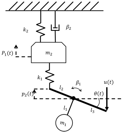
Figure 1.
Single link robot arm.
The robot has the following nonlinear model:
The measurable states are
The parameters considered are given in Table 1.

Table 1.
Parameters of model.
Taking as the states the position of , the linear speed of , the angle of the lever , the angular speed of the lever , and the position of the lever , we can represent the nonlinear model (51) as follows:
where is the semi-state vector , is the force input, and , are matrices containing nonlinear terms depending on the state variables. E is a singular constant matrix given as:
and C is a constant matrix
The variable terms presented in matrices , from the nonlinear model (51) are highlighted in boxes in Equations (57) and (58)
Considering the scheduling variables as
each variable has behavior limits depending on the variation of the input and the states.
Since there are two scheduling variables, then four weighting functions are obtained:
where and are the upper and lower limit of variation of , respectively, for all .
In this case , therefore there are membership functions, as:
Once the fuzzy sets are defined, the Takagi–Sugeno model has four rules. For each rule, there is a linear local model of the form:
For example, the first rule (65) corresponds to and then, lower limits are directly replaced by the nonlinear terms in matrices and , resulting in the following local model:
where and matrix E is defined in (55).
The Takagi–Sugeno model that reproduces the dynamics of the nonlinear model is given by:
where
The Takagi–Sugeno model of the single link robot arm is
Considering a constant input as , we can obtain the variation level of that allows us to determine the maximum and minimum of variation of and , to finally obtain the local matrices for the T-S model as:
and matrix C is given in (56).
8. Results
By following Algorithm 1, a Generalized Functional Observer can be designed. The matrix L was chosen in order to estimate the non-measurable state of the system.
Considering matrix , the matrix gains for the GFO are:
, ,
, , , , , , , ,
, , ,
, , , .
In order to compare the performance of the GFO, a PFO is also designed as a particular case. Considering matrix , the matrix gains for the PFO are:
, ,
, , , ,
, , , .
Considering a constant unit step input and, just in simulation, an additive parameter variation of the rigidity coefficient of spring 2, given as , where is presented in Figure 2. It is important to note that the generalized approach to the functional observer allows it to have different matrices as degrees of freedom as well as some robustness to parametric uncertainties. These uncertainties may come as a variation in the parameter values due to different physical processes, and may or may not be time-variant. In this example, we choose a time-varying uncertainty with a sinusoidal form. The generalized observer is capable of estimating the function with minor impact on performance.
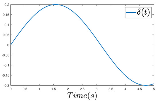
Figure 2.
Parametric uncertainty.
This parameter variation allows us to observe the robustness characteristics of the GFO compared with a simplest observer structure as the PFO.
The simulation is realized taking the input and output of the nonlinear system (53) and (54) in face to parametric uncertainty of Figure 2, the T-S system of (71) and (72) is just used for the observer design. Considering the initial conditions for the nonlinear system as and the initial condition for both observers as and , the results of the simulation are shown in Figure 3, Figure 4 and Figure 5.
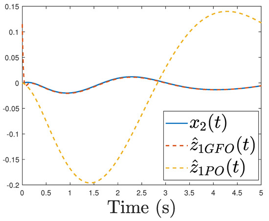
Figure 3.
and its estimates.
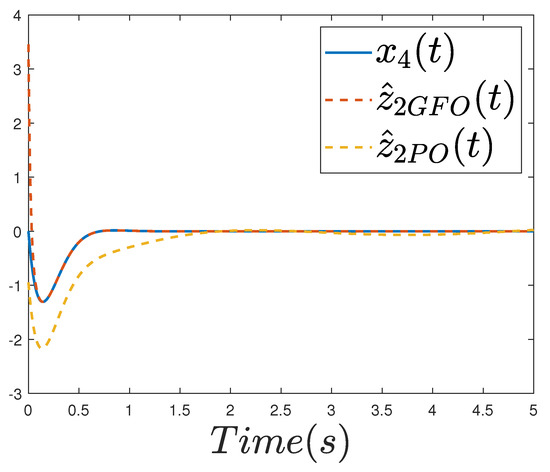
Figure 4.
and its estimates.
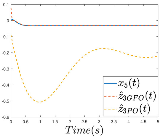
Figure 5.
and its estimates.
As can be seen in Figure 3, Figure 4 and Figure 5, the generalized observer is capable of estimating the state of the system even in the presence of parametric uncertainties. This presents an advantage compared to the classical proportional observers. The comparison between the performance of the genrealized observer and the Proportional observer is conducted through the error indexes which provide important information about the estimation error. For the case of a parametric uncertainty, the generalized approach outperforms the classical proportional observer. The error indexes of the Integral of the Absolute Error (IAE) and the Integral of the Time weighted Absolute Error (ITAE) are shown in Table 2.
Table 2.
Error indexes.
From Table 2, it can be seen that the proposed GFO exhibits better performance in comparison to the proportional observer. The generalized approach allows a better estimation of the function when parametric uncertainties are present in the system.
9. Conclusions
In this paper, a method for function estimation based on generalized observer for descriptor Takagi–Sugeno systems is presented. A function estimation can be used for two main objectives: The first, and used in the simulation example presented herein, is the estimation of the non-measurable states that could be considered as a reducer order observer, although an even smaller number of states could be estimated, given that the impulse functional observability presented in Assumption 1, is satisfied. The second objective for the function estimation is to estimate a control law based on the states without the need to estimate the states independently, but rather the function directly. The design and conditions of existence of the proposed observer were provided through a stability analysis based on Lyapunov. An example of a physical system was used to provide a comparison of the GFO with a PFO, both in the presence of parametric uncertainties. This paper can be extended in future works to include fault estimation, time delays, or to estimate a fault-tolerant control law. The descriptor approach of this paper can be used in future work since it is a powerful tool for representing a large number of mathematical systems.
Author Contributions
Conceptualization, C.R.-R., G.-L.O.-G. and M.D.; methodology, C.R.-R., G.-L.O.-G. and C.-M.A.-Z.; software, C.R.-R. and H.S.-A.; validation, C.R.-R., H.S.-A. and J.R.-R.; formal analysis, C.R.-R., G.-L.O.-G. and M.D.; investigation, C.R.-R., M.D. and C.-M.A.-Z.; writing—original draft preparation, C.R.-R., G.-L.O.-G. and H.S.-A.; writing—review and editing, C.R.-R., G.-L.O.-G., C.-M.A.-Z., M.D., H.S.-A. and J.R.-R.; supervision, G.-L.O.-G., C.-M.A.-Z. and M.D. All authors have read and agreed to the published version of the manuscript.
Funding
This research received no external funding.
Institutional Review Board Statement
Not applicable.
Informed Consent Statement
Not applicable.
Data Availability Statement
Not applicable.
Acknowledgments
The development of this project is the product of the support provided by the National Council of Science and Technology (CONACYT), the National Technological Institute of Mexico (TecNM)/CENIDET.
Conflicts of Interest
The authors declare no conflict of interest.
References
- Fernando, T.L.; Trinh, H.M.; Jennings, L. Functional observability and the design of minimum order linear functional observers. IEEE Trans. Autom. Control 2010, 55, 1268–1273. [Google Scholar] [CrossRef]
- Fernando, T.L.; Trinh, H.M. A system decomposition approach to the design of functional observers. Int. J. Control 2014, 87, 1846–1860. [Google Scholar] [CrossRef]
- Darouach, M. Existence and design of functional observers for linear systems. IEEE Trans. Autom. Control 2000, 45, 940–943. [Google Scholar] [CrossRef]
- Darouach, M. On the functional observers for linear descriptor systems. Syst. Control Lett. 2012, 61, 427–434. [Google Scholar] [CrossRef]
- Darouach, M.; Fernando, T.L. On the existence and design of functional observers. IEEE Trans. Autom. Control 2019, 65, 2751–2759. [Google Scholar] [CrossRef]
- Emami, K.; Fernando, T.L.; Nener, B.; Trinh, H.; Zhang, Y. A functional observer based fault detection technique for dynamical systems. J. Frankl. Inst. 2015, 352, 2113–2128. [Google Scholar] [CrossRef]
- Hamdoun, M.; Abdallah, M.B.; Ayadi, M.; Rotella, F.; Zambettakis, I. Functional observer-based feedback controller for ball balancing table. SN Appl. Sci. 2021, 3, 1–9. [Google Scholar] [CrossRef]
- Alhelou, H.H.; Golshan, M.E.H.; Hatziargyriou, N.D. A decentralized functional observer based optimal LFC considering unknown inputs, uncertainties, and cyber-attacks. IEEE Trans. Power Syst. 2019, 34, 4408–4417. [Google Scholar] [CrossRef]
- Koenig, D.; Marx, B.; Varrier, S. Filtering and fault estimation of descriptor switched systems. Automatica 2016, 63, 116–121. [Google Scholar] [CrossRef]
- Darouach, M.; Amato, F.; Alma, M. Functional observers design for descriptor systems via LMI: Continuous and discrete-time cases. Automatica 2017, 86, 216–219. [Google Scholar] [CrossRef]
- Ríos-Ruiz, C.; Osorio-Gordillo, G.L.; Souley-Ali, H.; Darouach, M.; Astorga-Zaragoza, C.M. Finite time functional observers for descriptor systems. Application to fault tolerant control. In Proceedings of the 2019 27th Mediterranean Conference on Control and Automation (MED), Akko, Israel, 1–4 July 2019; pp. 165–170. [Google Scholar]
- Zhang, J.; Wang, Z.; Chadli, M.; Wang, Y. On prescribed-time functional observers of linear descriptor systems with unknown input. Int. J. Control 2021, 1–16. [Google Scholar] [CrossRef]
- Huang, J.; Che, H.; Raissi, T.; Wang, Z. Functional Interval Observer for Discrete-time Switched Descriptor Systems. IEEE Trans. Autom. Control 2021. [Google Scholar] [CrossRef]
- Islam, S.I.; Lim, C.C.; Shi, P. Robust fault detection of TS fuzzy systems with time-delay using fuzzy functional observer. Fuzzy Sets Syst. 2020, 392, 1–23. [Google Scholar] [CrossRef]
- Islam, S.I.; Lim, C.C.; Shi, P. Functional observer based controller for stabilizing Takagi-Sugeno fuzzy systems with time-delays. J. Frankl. Inst. 2018, 355, 3619–3640. [Google Scholar] [CrossRef]
- Xie, W.B.; Wang, T.Z.; Lam, H.K.; Wang, X. Functional observer-controller method for unmeasured premise variables Takagi-Sugeno systems with external disturbance. Int. J. Syst. Sci. 2020, 51, 3436–3450. [Google Scholar] [CrossRef]
- Eltag, K.; Aslam, M.S.; Chen, Z. Functional Observer-Based T-S Fuzzy Systems for Quadratic Stability of Power System Synchronous Generator. Int. J. Fuzzy Syst. 2020, 22, 172–180. [Google Scholar] [CrossRef]
- Naifar, O.; Boukettaya, G.; Oualha, A.; Ouali, A. A comparative study between a high-gain interconnected observer and an adaptive observer applied to IM-based WECS. Eur. Phys. J. Plus 2015, 130, 1–13. [Google Scholar] [CrossRef]
- Ayadi, M.; Naifar, O.; Derbel, N. High-order sliding mode control for variable speed PMSG-wind turbine-based disturbance observer. Int. J. Model. Identif. Control 2019, 32, 85–92. [Google Scholar] [CrossRef]
- López-Estrada, F.R.; Theilliol, D.; Astorga-Zaragoza, C.M.; Ponsart, J.C.; Valencia-Palomo, G.; Camas-Anzueto, J. Fault diagnosis observer for descriptor Takagi-Sugeno systems. Neurocomputing 2019, 331, 10–17. [Google Scholar] [CrossRef]
- Nguyen, A.T.; Campos, V.; Guerra, T.M.; Pan, J.; Xie, W. Takagi-Sugeno fuzzy observer design for nonlinear descriptor systems with unmeasured premise variables and unknown inputs. Int. J. Robust Nonlinear Control 2021. [Google Scholar] [CrossRef]
- Zhang, J.; Zhu, F.; Karimi, H.R.; Wang, F. Observer-based sliding mode control for T-S fuzzy descriptor systems with time delay. IEEE Trans. Fuzzy Syst. 2019, 27, 2009–2023. [Google Scholar] [CrossRef]
- Jafari, E.; Binazadeh, T. Observer-based tracker design for discrete-time descriptor systems with constrained inputs. J. Process Control 2020, 94, 26–35. [Google Scholar] [CrossRef]
- Li, J.; Zhai, D. A descriptor regular form-based approach to observer-based integral sliding mode controller design. Int. J. Robust Nonlinear Control 2021, 31, 5134–5148. [Google Scholar] [CrossRef]
- Blandeau, M.; Guerra, T.M.; Pudlo, P. Application of a TS unknown input observer for studying sitting control for people living with spinal cord injury. In Control Applications for Biomedical Engineering Systems; Elsevier: Amsterdam, The Netherlands, 2020; pp. 169–195. [Google Scholar]
- Reyero-Santiago, P.; Ocampo-Martinez, C.; Braatz, R.D. Nonlinear Dynamical Analysis for an Ethanol Steam Reformer: A Singular Distributed Parameter System. In Proceedings of the 2020 59th IEEE Conference on Decision and Control (CDC), Virtual, 14–18 December 2020; pp. 23–29. [Google Scholar]
- Van Nguyen, T.; Ha, X.V. An Application of Observer Reconstruction to Estimate Actuator Fault for DC Motor Nonlinear System Under Effects of the Temperature and Disturbance. Furth. Adv. Internet Things Biomed. Cyber Phys. Syst. 2021, 55. [Google Scholar]
- Flores-Hernández, A.A.; Reyes-Reyes, J.; Astorga-Zaragoza, C.M.; Osorio-Gordillo, G.L.; García-Beltrán, C.D. Temperature control of an alcoholic fermentation process through the Takagi-Sugeno modeling. Chem. Eng. Res. Des. 2018, 140, 320–330. [Google Scholar] [CrossRef]
- Astorga-Zaragoza, C.M.; Osorio-Gordillo, G.L.; Reyes-Martínez, J.; Madrigal-Espinosa, G.; Chadli, M. Takagi—Sugeno observers as an alternative to nonlinear observers for analytical redundancy. application to a steam generator of a thermal power plant. Int. J. Fuzzy Syst. 2018, 20, 1756–1766. [Google Scholar] [CrossRef]
- Nguyen, A.T.; Dinh, T.Q.; Guerra, T.M.; Pan, J. Takagi-Sugeno fuzzy unknown input observers to estimate nonlinear dynamics of autonomous ground vehicles: Theory and real-time verification. IEEE/ASME Trans. Mechatron. 2021, 26, 1328–1338. [Google Scholar] [CrossRef]
- Flores-Martínez, M.A.; Osorio-Gordillo, G.L.; Vargas-Méndez, R.A.; Reyes-Reyes, J. Fuzzy functional observer for the control of the glucose-insulin system. J. Intell. Fuzzy Syst. 2019, 37, 5085–5096. [Google Scholar] [CrossRef]
- Chakrabarty, A.; Corless, M.J.; Buzzard, G.T.; Żak, S.H.; Rundell, A.E. State and unknown input observers for nonlinear systems with bounded exogenous inputs. IEEE Trans. Autom. Control 2017, 62, 5497–5510. [Google Scholar] [CrossRef]
- Skelton, R.E.; Iwasaki, T.; Grigoriadis, K. A Unified Algebraic Approach to Linear Control Design; Taylor & Francis: Abingdon, UK, 1998. [Google Scholar]
- Trinh, H.; Fernando, T. Functional Observers for Dynamical Systems; Springer Science & Business Media: Berlin, Germany, 2011; Volume 420. [Google Scholar]


Disclaimer/Publisher’s Note: The statements, opinions and data contained in all publications are solely those of the individual author(s) and contributor(s) and not of MDPI and/or the editor(s). MDPI and/or the editor(s) disclaim responsibility for any injury to people or property resulting from any ideas, methods, instructions or products referred to in the content. |
© 2023 by the authors. Licensee MDPI, Basel, Switzerland. This article is an open access article distributed under the terms and conditions of the Creative Commons Attribution (CC BY) license (https://creativecommons.org/licenses/by/4.0/).