

Pinch-Based General Targeting Method for Predicting the Optimal Capital Cost of Heat Exchanger Network

Abstract
1. Introduction
2. Problem Statement
2.1. Heat Exchanger Cost Categories
2.2. Non-Uniform Cost Laws of Heat Exchanger
2.3. Maximum Area Limitation for Heat Exchangers
3. General ESPA Method for Capital Cost Target
3.1. Establishment of the SPA Structure
3.1.1. Shifted BCCs
3.1.2. Division of Enthalpy Intervals
3.1.3. SPA Structure of HEN
3.2. Loop Elimination Principles
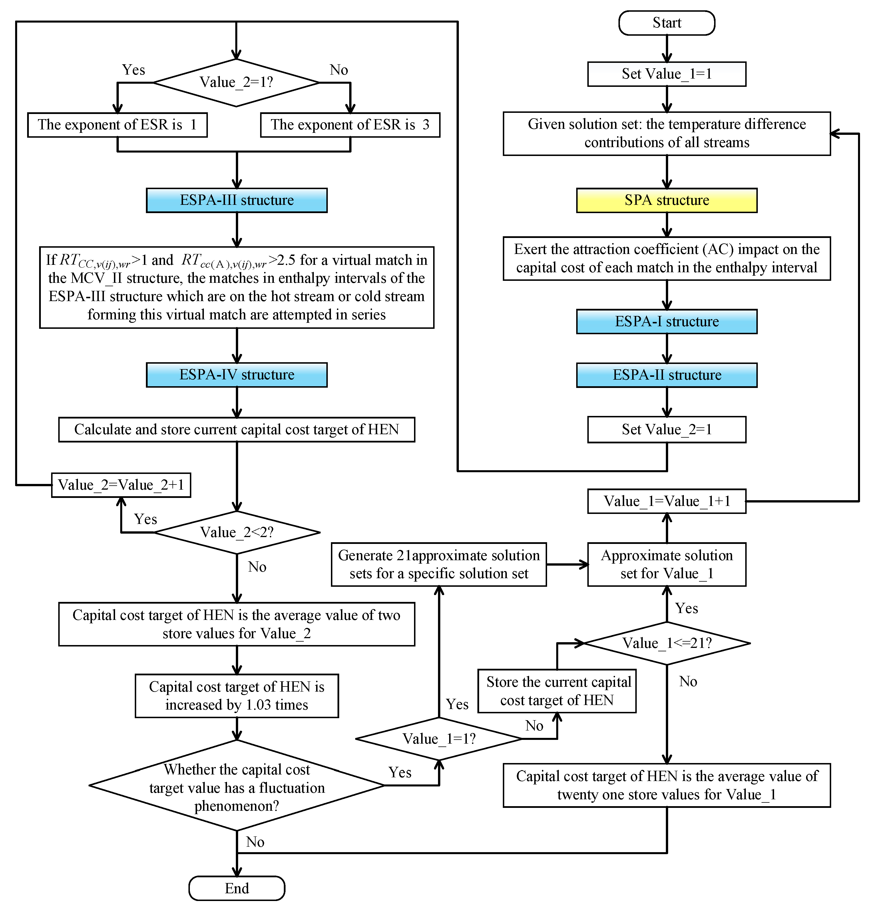
3.3. Evolution of ESPA Structures
3.3.1. Derivation of the ESPA-I Structure
3.3.2. Derivation of the ESPA-II Structure
3.3.3. Derivation of the ESPA-III Structure
3.3.4. Derivation of the ESPA-IV Structure
3.4. Target Value of Capital Cost for HEN
4. Accuracy Test and Analysis of General ESPA Method
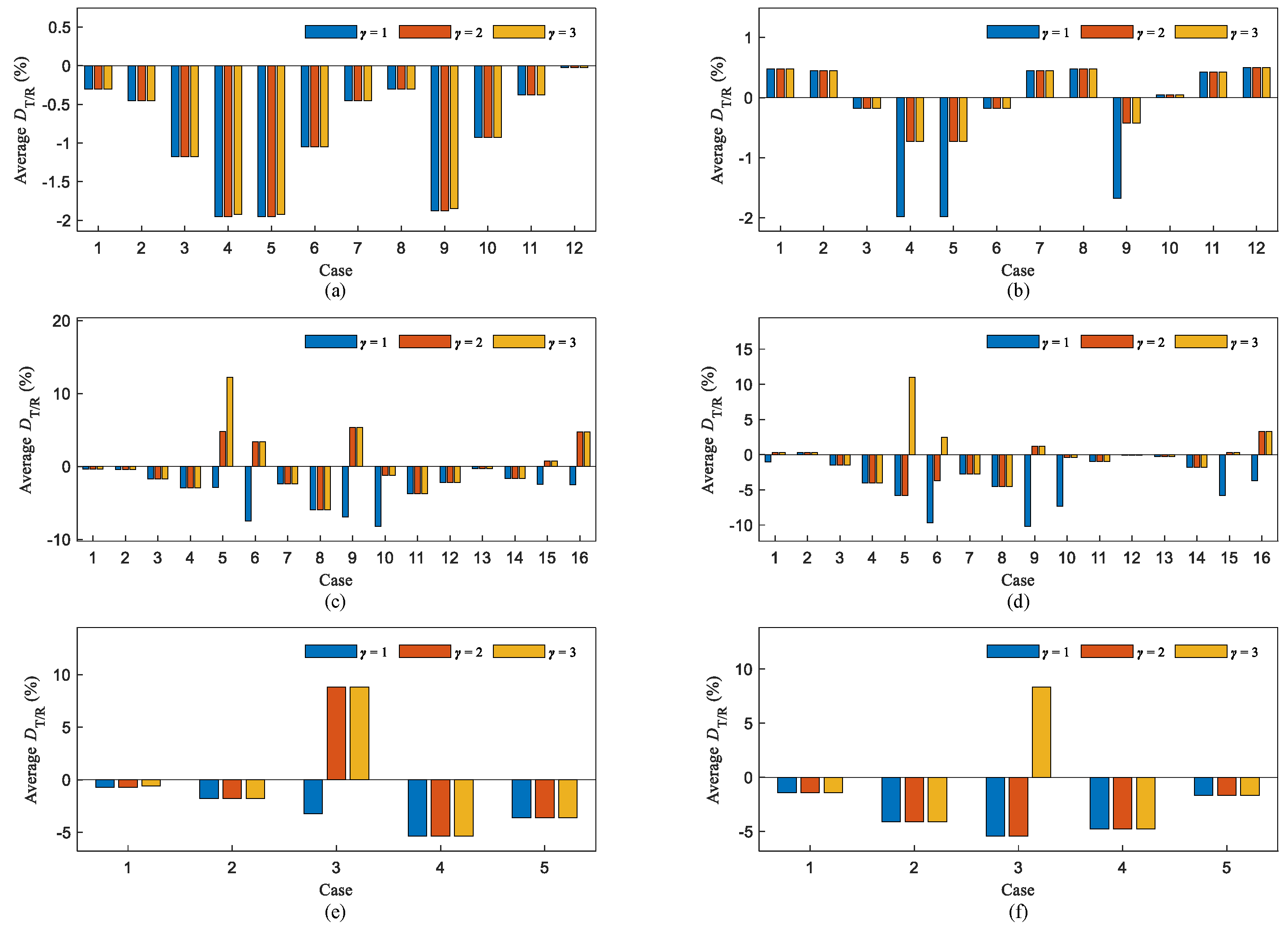
4.1. Accuracy Evaluation
4.2. Accuracy Test of General ESPA Method
4.3. Analysis and Improvement of the General ESPA Method
4.3.1. Measure for Enhancing Stability
4.3.2. Measure for Improving Accuracy
5. Optimization of the TDCs of Stream
5.1. Uniform TDCs for Streams
5.2. Individual TDCs for Streams
6. Case Studies
6.1. Case Study 1
6.2. Case Study 2
6.3. Case Study 3
6.4. Case Study 4
6.5. Accuracy Enhancement Measures
7. Discussion
7.1. Significance of Work
7.2. Limitations of Work
8. Conclusions
- (1)
- The proposed targeting method has wide applicability. As required, this targeting method can flexibly impose area limitations, freely set HECCs for stream pairs, or apply non-uniform cost laws for a particular stream pair.
- (2)
- The prediction capacity of the targeting method was enhanced. The use of individual stream TDCs is allowed for the targeting method, achieving more cost prediction possibilities. The effects of optimizing the individual stream TDCs are demonstrated in case studies.
- (3)
- Excellent target accuracy is verified. The absolute deviations between capital cost targets and reference capital costs are less than 10% in all numerical experiments and often less than 5%. The absolute target deviations were the same in case studies where the best HEN cost results in the literature were used as references.
- (4)
- The cost target derived by applying the general ESPA method can be used as a benchmark to guide the synthesis of HEN and evaluate the quality of the designed HEN. If the capital cost of HEN is 10% higher than the target value, the HEN synthesis is very likely to need improvement. Improving the designed HEN further would be difficult when the capital cost of HEN is close to the value of 10% lower than the target result.
Supplementary Materials
Author Contributions
Funding
Institutional Review Board Statement
Informed Consent Statement
Data Availability Statement
Conflicts of Interest
Nomenclature
| variables | |
| A | Area of heat exchange |
| CC | Capital cost |
| cc | Capital cost per unit energy or area |
| CP | Heat capacity flow rate |
| DT/R | Capital cost target deviation |
| E | Indication of the existence of a match |
| FT | LMTD correction factor |
| h | Heat transfer coefficient of the stream |
| Nshell | Number of shells in series |
| q | Heat exchange load between streams |
| RC | Reference cost |
| RT | Ratio value |
| ΔTLM | Logarithmic mean temperature difference |
| parameters | |
| a, b, c | Cost parameters of heat exchanger specification |
| γ | Exponent of ESR |
| indexes | |
| C | Cold stream |
| cont | Contribution |
| H | Hot stream |
| i | Index of hot stream |
| ir | Independent region |
| j | Index of cold stream |
| k | Index of enthalpy interval |
| l | Index of heat exchanger specification |
| m | Heat exchange match |
| RC | Reference cost |
| se | Sub-cost law |
| TC | Target cost |
| U | Heat exchange unit |
| v | Virtual match |
| wr | Whole region |
| x | One certain segment of heat exchanger unit |
| z | Index of the enthalpy interval that forms a virtual match |
| abbreviations | |
| AC | Attraction coefficient |
| ATM | Automated targeting model |
| BCC | Balanced composite curve |
| ESR | Energy shift ratio |
| ESPA | Evolved from the spaghetti structure |
| GA | Genetic algorithm |
| HECC | Heat exchanger cost category |
| HEN | Heat exchanger network |
| LMTD | Logarithmic mean temperature difference |
| MTD | Minimum temperature difference |
| PTD | Pinch temperature difference |
| SIR | Structure identification and change of reference system |
| SPA | Spaghetti |
| TDC | Temperature difference contribution |
| TDF | Temperature driving force |
References
- Sun, X.; Zhuang, Y.; Liu, L.; Dong, Y.; Zhang, L.; Du, J. Multi-objective optimization of heat exchange network and thermodynamic cycles integrated system for cooling and power cogeneration. Appl. Energy 2022, 321, 119366. [Google Scholar] [CrossRef]
- Fieg, G.; Luo, X.; Jezowski, J. A monogenetic algorithm for optimal design of large-scale heat exchanger networks. Chem. Eng. Process. Process Intensif. 2009, 48, 1506–1516. [Google Scholar] [CrossRef]
- Xiao, Y.; Sun, T.; Cui, G. Enhancing strategy promoted by large step length for the structure optimization of heat exchanger networks. Appl. Therm. Eng. 2020, 173, 115199. [Google Scholar] [CrossRef]
- Xiao, Y.; Cui, G.; Zhang, G.; Ai, L. Parallel optimization route promoted by accepting imperfect solutions for the global optimization of heat exchanger networks. J. Cleaner Prod. 2022, 336, 130354. [Google Scholar] [CrossRef]
- Xu, Y.; Cui, G.; Han, X.; Xiao, Y.; Zhang, G. Optimization route arrangement: A new concept to achieve high efficiency and quality in heat exchanger network synthesis. Int. J. Heat Mass Transfer 2021, 178, 121622. [Google Scholar] [CrossRef]
- Rathjens, M.; Fieg, G. A novel hybrid strategy for cost-optimal heat exchanger network synthesis suited for large-scale problems. Appl. Therm. Eng. 2020, 167, 114771. [Google Scholar] [CrossRef]
- Feyli, B.; Soltani, H.; Hajimohammadi, R.; Fallahi-Samberan, M.; Eyvazzadeh, A. A reliable approach for heat exchanger networks synthesis with stream splitting by coupling genetic algorithm with modified quasi-linear programming method. Chem. Eng. Sci. 2022, 248, 117140. [Google Scholar] [CrossRef]
- Xiao, Y.; Kayange, H.A.; Cui, G.; Li, W. Node dynamic adaptive non-structural model for efficient synthesis of heat exchanger networks. J. Cleaner Prod. 2021, 296, 126552. [Google Scholar] [CrossRef]
- Bayomie, O.S.; Abdelaziz, O.Y.; Gadalla, M.A. Exceeding Pinch limits by process configuration of an existing modern crude oil distillation unit—A case study from refining industry. J. Clean. Prod. 2019, 231, 1050–1058. [Google Scholar] [CrossRef]
- Bandyopadhyay, R.; Alkilde, O.F.; Upadhyayula, S. Applying pinch and exergy analysis for energy efficient design of diesel hydrotreating unit. J. Clean. Prod. 2019, 232, 337–349. [Google Scholar] [CrossRef]
- Wang, M.; Deng, C.; Wang, Y.; Feng, X. Exergoeconomic performance comparison, selection and integration of industrial heat pumps for low grade waste heat recovery. Energy Convers. Manage. 2020, 207, 112532. [Google Scholar] [CrossRef]
- Ghorbani, B.; Ebrahimi, A.; Rooholamini, S.; Ziabasharhagh, M. Pinch and exergy evaluation of Kalina/Rankine/gas/steam combined power cycles for tri-generation of power, cooling and hot water using liquefied natural gas regasification. Energy Convers. Manage. 2020, 223, 113328. [Google Scholar] [CrossRef]
- Liu, S.; Yang, L.; Chen, B.; Yang, S.; Qian, Y. Comprehensive energy analysis and integration of coal-based MTO process. Energy 2021, 214, 119060. [Google Scholar] [CrossRef]
- Langner, C.; Svensson, E.; Harvey, S. A computational tool for guiding retrofit projects of industrial heat recovery systems subject to variation in operating conditions. Appl. Therm. Eng. 2021, 182, 115648. [Google Scholar] [CrossRef]
- Asante, N.D.K.; Zhu, X.X. An automated and interactive approach for heat exchanger network retrofit. Chem. Eng. Res. Des. 1997, 75, 349–360. [Google Scholar] [CrossRef]
- Wang, B.; Klemeš, J.J.; Li, N.; Zeng, M.; Varbanov, P.S.; Liang, Y. Heat exchanger network retrofit with heat exchanger and material type selection: A review and a novel method. Renew. Sustain. Energy Rev. 2021, 138, 110479. [Google Scholar] [CrossRef]
- Gundersen, T.; Grossmann, I.E. Improved optimization strategies for automated heat exchanger network synthesis through physical insights. Comput. Chem. Eng. 1990, 14, 925–944. [Google Scholar] [CrossRef]
- Ahmad, S.; Linnhoff, B.; Smith, R. Cost optimum heat exchanger networks—2. Targets and design for detailed capital cost models. Comput. Chem. Eng. 1990, 14, 751–767. [Google Scholar] [CrossRef]
- Jegede, F.O.; Polley, G.T. Capital cost targets for networks with non-uniform heat exchanger specifications. Comput. Chem. Eng. 1992, 16, 477–495. [Google Scholar] [CrossRef]
- Serna-González, M.; Jiménez-Gutiérrez, A.; Ponce-Ortega, J.M. Targets for heat exchanger network synthesis with different heat transfer coefficients and non-uniform exchanger specifications. Chem. Eng. Res. Des. 2007, 85, 1447–1457. [Google Scholar] [CrossRef]
- Akbarnia, M.; Amidpour, M.; Shadaram, A. A new approach in pinch technology considering piping costs in total cost targeting for heat exchanger network. Chem. Eng. Res. Des. 2009, 87, 357–365. [Google Scholar] [CrossRef]
- Serna-González, M.; Ponce-Ortega, J.M. Total cost target for heat exchanger networks considering simultaneously pumping power and area effects. Appl. Therm. Eng. 2011, 31, 1964–1975. [Google Scholar] [CrossRef]
- Diban, P.; Foo, D.C.Y. A pinch-based automated targeting technique for heating medium system. Energy 2019, 166, 193–212. [Google Scholar] [CrossRef]
- Ulyev, L.; Boldyryev, S.; Kuznetsov, M. Investigation of process stream systems for targeting energy-capital trade-offs of a heat recovery network. Energy 2023, 263, 125954. [Google Scholar] [CrossRef]
- Fu, D.; Nguyen, T.; Lai, Y.; Lin, L.; Dong, Z.; Lyu, M. Improved pinch-based method to calculate the capital cost target of heat exchanger network via evolving the spaghetti structure towards low-cost matching. J. Cleaner Prod. 2022, 343, 131022. [Google Scholar] [CrossRef]
- Jiang, N.; Shelley, J.D.; Doyle, S.; Smith, R. Heat exchanger network retrofit with a fixed network structure. Appl. Energy 2014, 127, 25–33. [Google Scholar] [CrossRef]
- Kemp, I.C. Pinch Analysis and Process Integration: A User Guide on Process Integration for the Efficient Use of Energy, 2nd ed.; Elsevier: Oxford, UK, 2007. [Google Scholar]
- Jiang, N.; Bao, S.; Gao, Z. Heat Exchanger Network Integration Using Diverse Pinch Point and Mathematical Programming. Chem. Eng. Technol. 2011, 34, 985–990. [Google Scholar] [CrossRef]
- Bowman, R.A.; Mueller, A.C.; Nagle, W.M. Mean temperature difference in design. Trans. ASME 1940, 62, 283–294. [Google Scholar] [CrossRef]
- Smith, R. Chemical Process Design and Integration; Wiley: Chichester, UK, 2005; ISBN 0471486817. [Google Scholar]
- Dehghani, M.J.; Yoo, C. Three-step modification and optimization of Kalina power-cooling cogeneration based on energy, pinch, and economics analyses. Energy 2020, 205, 118069. [Google Scholar] [CrossRef]
- Galli, M.R.; Cerdá, J. Synthesis of heat exchanger networks featuring a minimum number of constrained-size shells of 1-2 type. Appl. Therm. Eng. 2000, 20, 1443–1467. [Google Scholar] [CrossRef]
- Chauhan, S.S.; Khanam, S. Simultaneous water and energy conservation in non-isothermal processes—A case study of thermal power plant. J. Clean. Prod. 2021, 282, 125423. [Google Scholar] [CrossRef]
- Ponce-Ortega, J.M.; Serna-González, M.; Jiménez-Gutiérrez, A. Synthesis of multipass heat exchanger networks using genetic algorithms. Comput. Chem. Eng. 2008, 32, 2320–2332. [Google Scholar] [CrossRef]
- Kayange, H.A.; Cui, G.; Xu, Y.; Li, J.; Xiao, Y. Non-structural model for heat exchanger network synthesis allowing for stream splitting. Energy 2020, 201, 117461. [Google Scholar] [CrossRef]
- Pavão, L.V.; Costa, C.B.B.; Ravagnani, M.A.S.S. A new stage-wise superstructure for heat exchanger network synthesis considering substages, sub-splits and cross flows. Appl. Therm. Eng. 2018, 143, 719–735. [Google Scholar] [CrossRef]
- Khorasany, R.M.; Fesanghary, M. A novel approach for synthesis of cost-optimal heat exchanger networks. Comput. Chem. Eng. 2009, 33, 1363–1370. [Google Scholar] [CrossRef]
- Zhaoyi, H.; Liang, Z.; Hongchao, Y.; Jianxiong, Y. Simultaneous synthesis of structural-constrained heat exchanger networks with and without stream splits. Can. J. Chem. Eng. 2013, 91, 830–842. [Google Scholar] [CrossRef]
- Pavão, L.V.; Costa, C.B.B.; Ravagnani, M.A.S.S. Heat Exchanger Network Synthesis without stream splits using parallelized and simplified simulated Annealing and Particle Swarm Optimization. Chem. Eng. Sci. 2017, 158, 96–107. [Google Scholar] [CrossRef]
- Zhang, H.; Cui, G.; Xiao, Y.; Chen, J. A novel simultaneous optimization model with efficient stream arrangement for heat exchanger network synthesis. Appl. Therm. Eng. 2017, 110, 1659–1673. [Google Scholar] [CrossRef]
- Chen, J.; Cui, G.; Duan, H. Multipopulation differential evolution algorithm based on the opposition-based learning for heat exchanger network synthesis. Numeri. Heat Transf. A Appl. 2017, 72, 126–140. [Google Scholar] [CrossRef]
- Zhang, H.; Cui, G. Optimal heat exchanger network synthesis based on improved cuckoo search via Levy flights. Chem. Eng. Res. Des. 2018, 134, 62–79. [Google Scholar] [CrossRef]
- Pavão, L.V.; Costa, C.B.B.; Ravagnani, M.A.S.S. An Enhanced Stage-wise Superstructure for Heat Exchanger Networks Synthesis with New Options for Heaters and Coolers Placement. Ind. Eng. Chem. Res. 2018, 57, 2560–2573. [Google Scholar] [CrossRef]
- Bao, Z.; Cui, G.; Chen, J.; Sun, T.; Xiao, Y. A novel random walk algorithm with compulsive evolution combined with an optimum-protection strategy for heat exchanger network synthesis. Energy 2018, 152, 694–708. [Google Scholar] [CrossRef]
- Xiao, Y.; Kayange, H.A.; Cui, G.; Chen, J. Non-structural model of heat exchanger network: Modeling and optimization. Int. J. Heat Mass Transfer 2019, 140, 752–766. [Google Scholar] [CrossRef]
- Björk, K.-M.; Pettersson, F. Optimization of large-scale heat exchanger network synthesis problems. Modell. Simul. 2003, 2003, 313–318. [Google Scholar]
- Pettersson, F. Synthesis of large-scale heat exchanger networks using a sequential match reduction approach. Comput. Chem. Eng. 2005, 29, 993–1007. [Google Scholar] [CrossRef]
- Luo, X.; Fieg, G.; Cai, K.; Guan, X. Synthesis of Large-Scale Heat Exchanger Networks by a Monogenetic Algorithm. In 10th International Symposium on Process Systems Engineering: Part A; Elsevier: Amsterdam, The Netherlands, 2009; ISBN 9780444534729. [Google Scholar]
- Ernst, P.; Fieg, G.; Luo, X. Efficient synthesis of large-scale heat exchanger networks using monogenetic algorithm. Heat Mass Transfer 2010, 46, 1087–1096. [Google Scholar] [CrossRef]
- Huang, K.F.; Karimi, I.A. Efficient algorithm for simultaneous synthesis of heat exchanger networks. Chem. Eng. Sci. 2014, 105, 53–68. [Google Scholar] [CrossRef]
- Zhang, C.; Cui, G.; Chen, S. An efficient method based on the uniformity principle for synthesis of large-scale heat exchanger networks. Appl. Therm. Eng. 2016, 107, 565–574. [Google Scholar] [CrossRef]
- Pavão, L.V.; Costa, C.B.B.; Ravagnani, M.A.D.S.S.; Jiménez, L. Large-Scale Heat Exchanger Networks Synthesis Using Simulated Annealing and the Novel Rocket Fireworks Optimization. AlChE J. 2017, 63, 1582–1601. [Google Scholar] [CrossRef]
- Xiao, Y.; Cui, G.; Sun, T.; Chen, J. An integrated random walk algorithm with compulsive evolution and fine-search strategy for heat exchanger network synthesis. Appl. Therm. Eng. 2018, 128, 861–876. [Google Scholar] [CrossRef]
- Nemet, A.; Isafiade, A.J.; Klemeš, J.J.; Kravanja, Z. Two-step MILP/MINLP approach for the synthesis of large-scale HENs. Chem. Eng. Sci. 2019, 197, 432–448. [Google Scholar] [CrossRef]
- Xiao, Y.; Kayange, H.A.; Cui, G. Heat integration of energy system using an integrated node-wise non-structural model with uniform distribution strategy. Int. J. Heat Mass Transf. 2020, 152, 119497. [Google Scholar] [CrossRef]
- Zhang, H.; Huang, X.; Peng, F.; Cui, G.; Huang, T. A novel two-step synthesis method with weakening strategy for solving large-scale heat exchanger networks. J. Clean. Prod. 2020, 275, 123103. [Google Scholar] [CrossRef]
- Smith, R.; Jobson, M.; Chen, L. Recent development in the retrofit of heat exchanger networks. Appl. Therm. Eng. 2010, 30, 2281–2289. [Google Scholar] [CrossRef]


| HECC | Cost Equation | Area Equation |
|---|---|---|
| A | Equation (1) | Equation (3) |
| B | Equation (1) | Equation (4) |
| C | Equation (2) | Equation (3) |
| D | Equation (2) | Equation (4) |
| Heat Exchanger Specification | Cost Law | HECC | Temperature Range | Cost Parameters | ||
|---|---|---|---|---|---|---|
| l | CL-0 (Default) | A/B/C/D | al−0 | bl−0 | cl−0 | |
| CL-1 (Hot) | A/B/C/D | [Tmin−1, Tmax−1] | al−1 | bl−1 | cl−1 | |
| CL-2 (Cold) | A/B/C/D | [Tmin−2, Tmax−2] | al−2 | bl−2 | cl−2 | |
| … | … | … | … | … | … | |
| Case | Optimal Cost | Uniform TDCs | Individual TDCs | Amax Limitation | Location | ||
|---|---|---|---|---|---|---|---|
| Cost Target | Cost Deviation | Cost Target | Cost Deviation | ||||
| 1 (a) | 263,854 $ | 262,510 $ | / | 241,131 $ | −8.61% | No | Figure 6a |
| 1 (b) | 267,747 $ | 267,054 $ | / | 251,503 $ | −6.07% | Yes | Figure 6b |
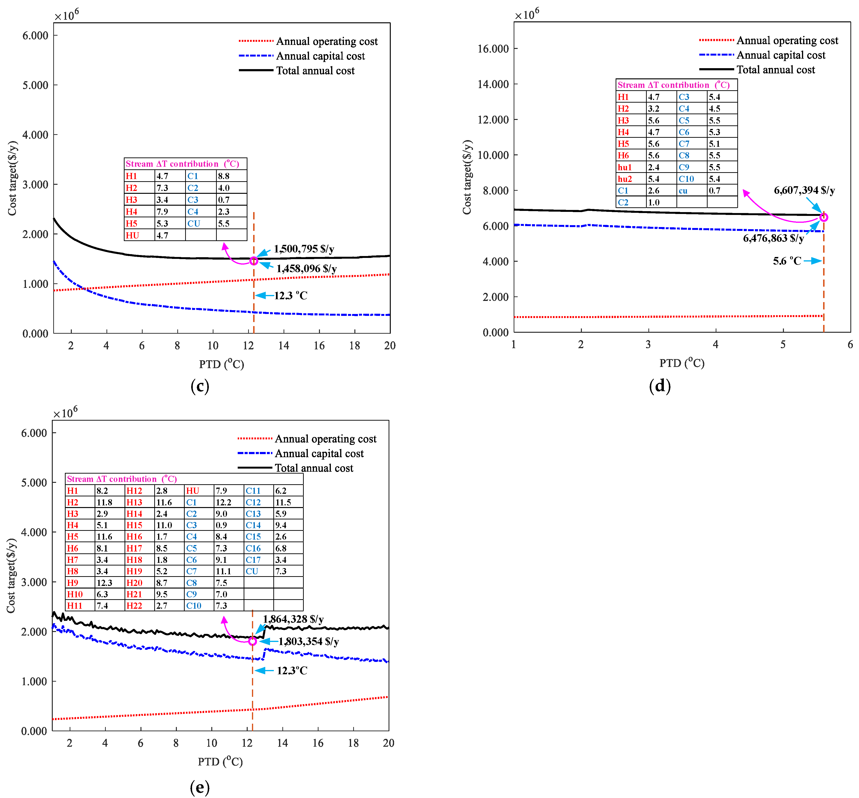
| 2 | 1,517,678 $/y | 1,500,795 $/y | −1.1% | 1,458,096 $/y | / | No | Figure 6c |
| 3 | 6,712,551 $/y | 6,607,394 $/y | / | 6,476,863 $/y | −3.5% | No | Figure 6d |
| 4 | 1,852,723 $/y | 1,864,328 $/y | / | 1,803,354 $/y | −2.7% | No | Figure 6e |
| Author | Ref. | Total Annual Cost ($/y) |
|---|---|---|
| Khorasany and Fesanghary (2009) | [37] | 7,435,740 |
| Huo Zhaoyi et al. (2013) | [38] | 7,361,190 |
| Pavão et al. (2017a) | [39] | 7,301,437 |
| Zhang et al. (2017) | [40] | 7,212,115 |
| Chen et al. (2017) | [41] | 6,989,989 |
| Zhang and Cui (2018) | [42] | 6,861,111 |
| Pavão et al. (2018) | [43] | 6,801,261 |
| Pavão et al. (2018) | [36] | 6,712,551 |
| Bao et al. (2018) | [44] | 6,869,610 |
| Xiao et al. (2019) | [45] | 6,798,067 |
| Kayange et al. (2020) | [35] | 6,716,343 |
| Author | Ref. | Total Annual Cost ($/y) |
|---|---|---|
| Björk and Pettersson (2003) | [46] | 2,073,251 |
| Pettersson (2005) | [47] | 1,997,054 |
| Luo et al. (2009) | [48] | 1.965 × 10⁶ |
| Ernst et al. (2010) | [49] | 1,943,536 |
| Huang and Karimi (2014) | [50] | 1,937,377 |
| Zhang et al. (2016) | [51] | 1,939,149 |
| Pavão et al. (2017) | [52] | 1,900,614 |
| Xiao et al. (2018) | [53] | 1,936,288 |
| Nemet et al. (2019) | [54] | 1.9288 × 10⁶ |
| Xiao et al. (2019) | [45] | 1,925,783 |
| Xiao et al. (2020) | [55] | 1,921,639 |
| Xiao et al. (2020) | [3] | 1,873,813 |
| Zhang et al. (2020) | [56] | 1,918,593 |
| Rathjens and Fieg (2020) | [6] | 1,852,913 |
| Xiao et al. (2021) | [8] | 1,910,630 |
| Xu et al. (2021) | [5] | 1,852,723 |
Disclaimer/Publisher’s Note: The statements, opinions and data contained in all publications are solely those of the individual author(s) and contributor(s) and not of MDPI and/or the editor(s). MDPI and/or the editor(s) disclaim responsibility for any injury to people or property resulting from any ideas, methods, instructions or products referred to in the content. |
© 2023 by the authors. Licensee MDPI, Basel, Switzerland. This article is an open access article distributed under the terms and conditions of the Creative Commons Attribution (CC BY) license (https://creativecommons.org/licenses/by/4.0/).
Share and Cite
Fu, D.; Li, Q.; Li, Y.; Lai, Y.; Lu, L.; Dong, Z.; Lyu, M. Pinch-Based General Targeting Method for Predicting the Optimal Capital Cost of Heat Exchanger Network. Processes 2023, 11, 923. https://doi.org/10.3390/pr11030923
Fu D, Li Q, Li Y, Lai Y, Lu L, Dong Z, Lyu M. Pinch-Based General Targeting Method for Predicting the Optimal Capital Cost of Heat Exchanger Network. Processes. 2023; 11(3):923. https://doi.org/10.3390/pr11030923
Chicago/Turabian StyleFu, Dianliang, Qixuan Li, Yan Li, Yanhua Lai, Lin Lu, Zhen Dong, and Mingxin Lyu. 2023. "Pinch-Based General Targeting Method for Predicting the Optimal Capital Cost of Heat Exchanger Network" Processes 11, no. 3: 923. https://doi.org/10.3390/pr11030923
APA StyleFu, D., Li, Q., Li, Y., Lai, Y., Lu, L., Dong, Z., & Lyu, M. (2023). Pinch-Based General Targeting Method for Predicting the Optimal Capital Cost of Heat Exchanger Network. Processes, 11(3), 923. https://doi.org/10.3390/pr11030923