Training Feedforward Neural Networks Using an Enhanced Marine Predators Algorithm
Abstract
1. Introduction
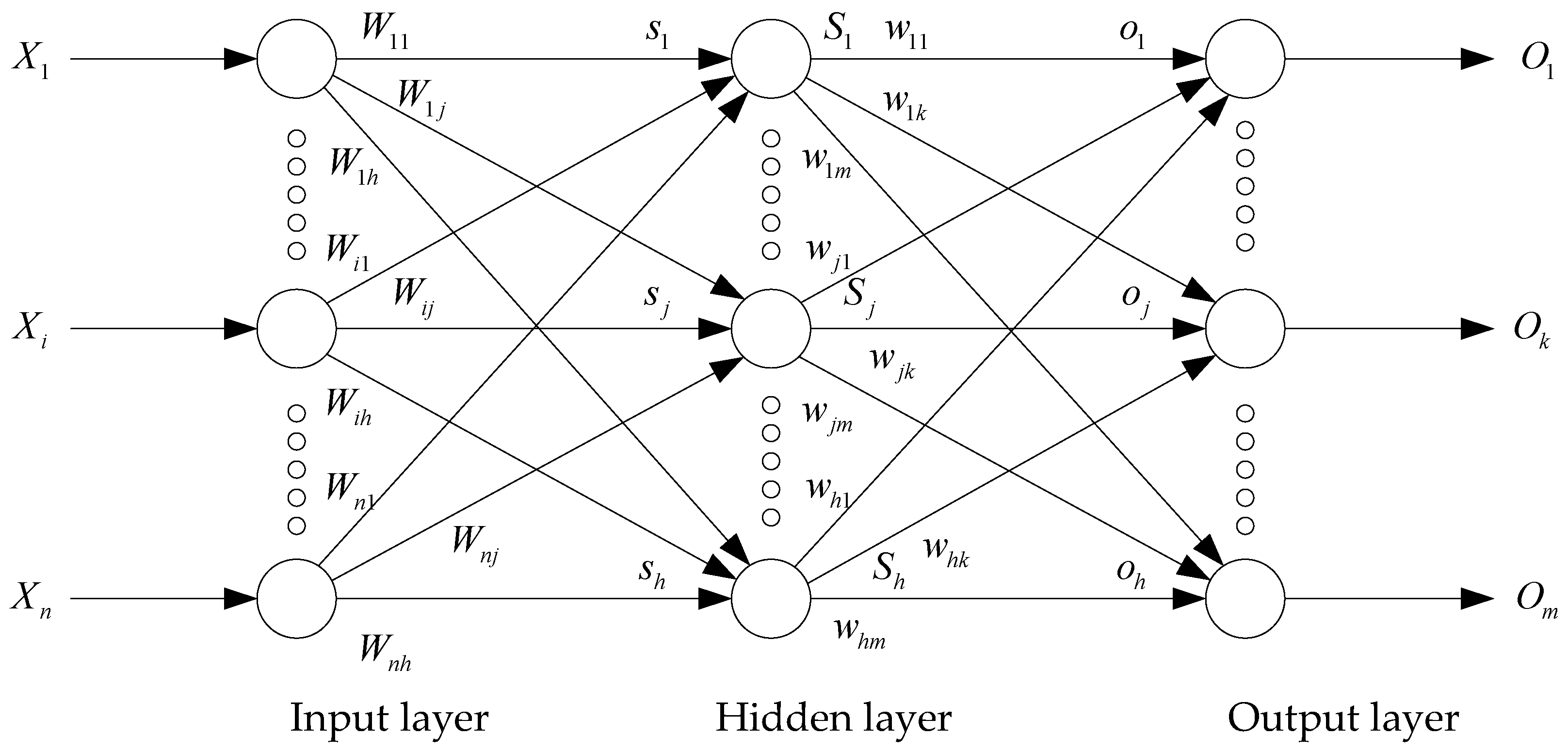
2. Mathematical Modeling of FNNs
3. MPA
3.1. Initialization
3.2. MPA Optimization Scenarios
3.3. Eddy Formation and FAD’s Effect
| Algorithm 1: MPA |
| Begin Step 1. Initialize the marine predator population and control parameters Step 2. Assess the fitness value of each predator Discover the ideal predator Step 3. while () do for each predator Construct the Elite and prey matrices via Equations (6) and (7) If Renew prey via Equations (9) and (10) Else if For the first half of the population quality Renew prey via Equations (12) and (13) For the other half of the population quality Renew prey via Equations (14) and (15) Else if Renew prey via Equations (18) and (19) End if Identify and amend any predator that travels beyond the search scope Complete memory conserving and Elite Renew Utilizing effect and renewing prey via Equation (20) Return the best predator End |
4. EMPA
| Algorithm 2: Ranking-based mutation operator of “DE/rand/1” |
| Begin Sort the population, and assign the ranking and selection probability for each predator Randomly select {base vector index} while Randomly select end Randomly select {terminal vector index} while Randomly select end Randomly select {starting vector index} while Randomly select end End |
| Algorithm 3: EMPA |
| Begin Step 1. Initialize the marine predator population and control parameters Step 2. Assess the fitness value of each predator Discover the ideal predator Step 3. while () do for each predator Sort the population; assign the ranking and selection probability for each predator /*ranking-based mutation stage*/ Randomly select {base vector index} while Randomly select end Randomly select {terminal vector index} while Randomly select end Randomly select {starting vector index} while Randomly select end /*end of ranking-based mutation stage*/ Construct the Elite and prey matrices via Equations (6) and (7) If Renew prey via Equations (9) and (10) Else if For the first half of the population quality Renew prey via Equations (12) and (13) For the other half of the population quality Renew prey via Equations (14) and (15) Else if Renew prey via Equations (18) and (19) End if Identify and amend any predator that travels beyond the search scope Complete memory conserving and Elite Renew Utilizing effect and renewing prey via Equation (20) Return the best predator End |
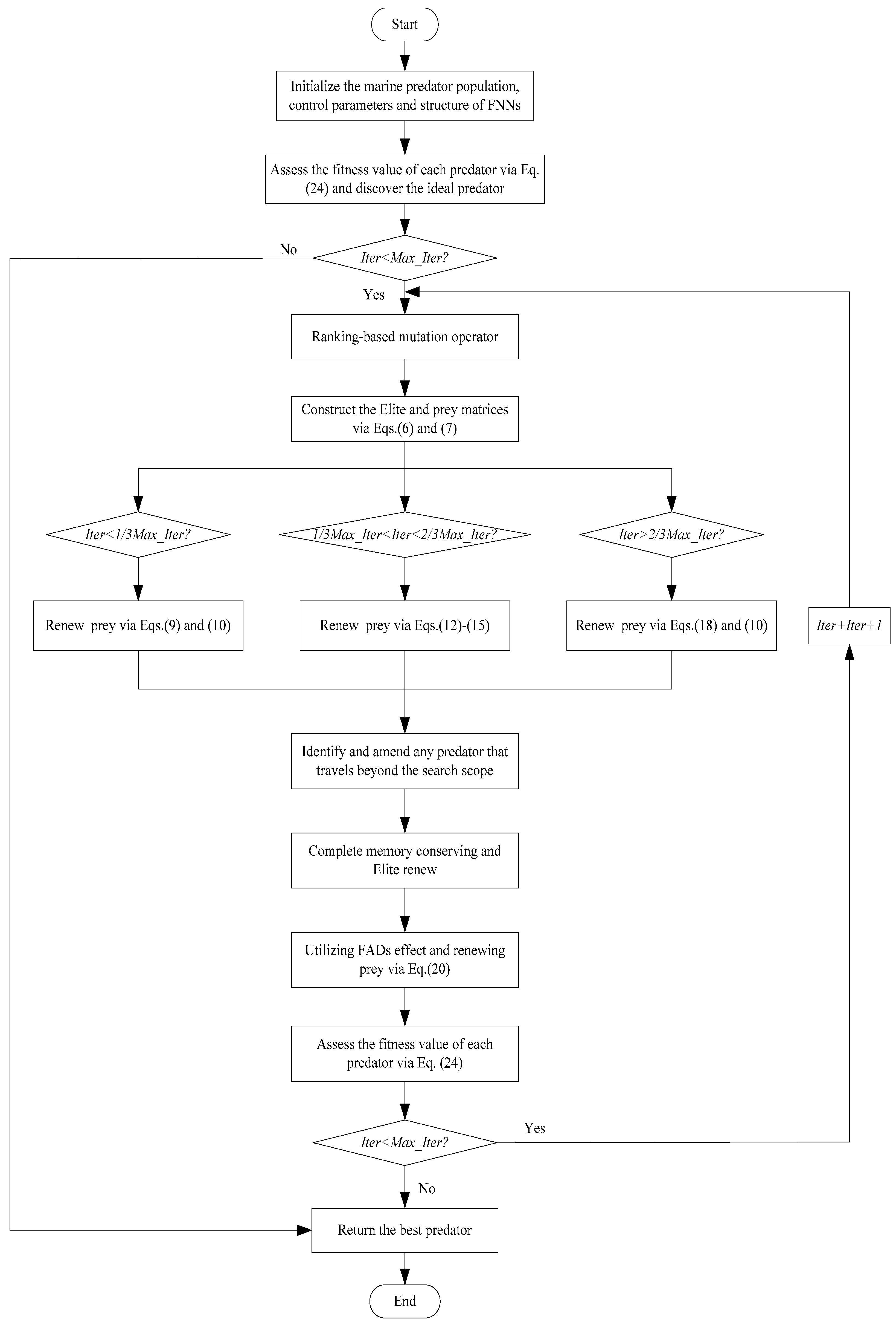
5. EMPA-Based Feedforward Neural Networks
| Algorithm 4: EMPA-based feedforward neural networks |
| Begin Step 1. Initialize the marine predator population , control parameters, and the structure of FNNs; each predator denotes the connection weight and deviation value Step 2. Assess the fitness value of each predator via Equation (24); assign connection weight to the predator Discover the ideal predator Step 3. while () do for each predator Sort the population; assign the ranking and selection probability for each predator /*ranking-based mutation stage*/ Randomly select {base vector index} while Randomly select end Randomly select {terminal vector index} while Randomly select end Randomly select {starting vector index} while Randomly select end /*end of ranking-based mutation stage*/ Construct the Elite and prey matrices via Equations (6) and (7) If Renew prey via Equations (9) and (10) Else if For the first half of the population quality Renew prey via Equations (12) and (13) For the other half of the population quality Renew prey via Equations (14) and (15) Else if Renew prey via Equations (18) and (19) End if Identify and amend any predator that travels beyond the search scope Complete memory conserving and Elite Renew Utilizing effect and renewing prey via Equation (20), and assessing the fitness value of each predator via Equation (24) Return the best predator End |
Complexity Analysis
6. Experimental Results and Analysis
6.1. Experimental Setup
6.2. Test Datasets
6.3. Parameter Setting
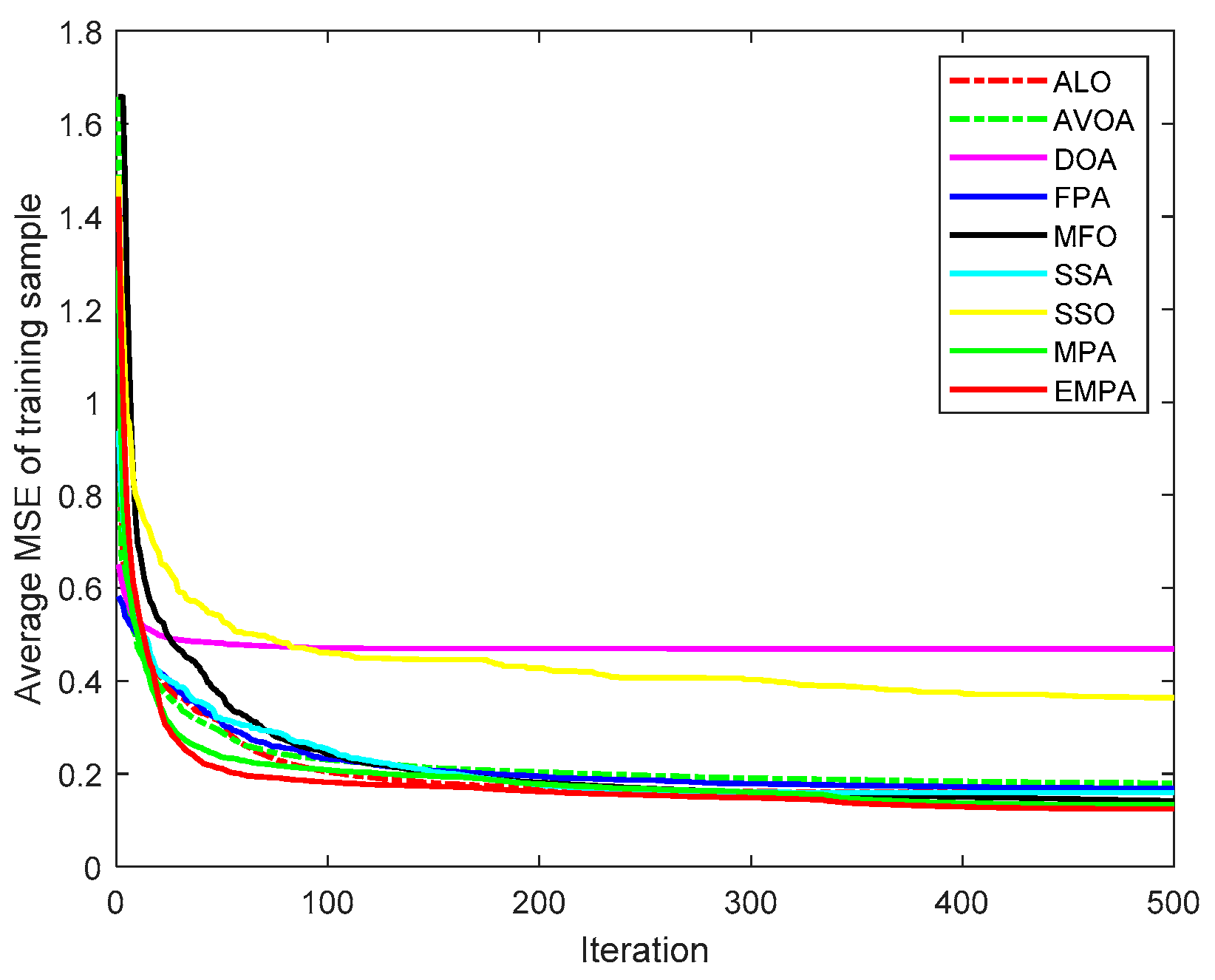
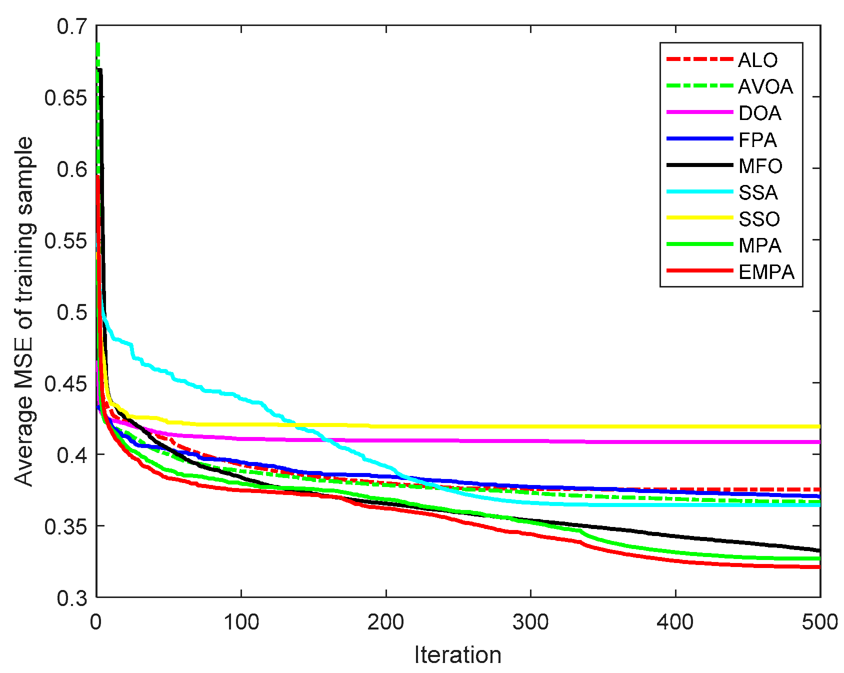
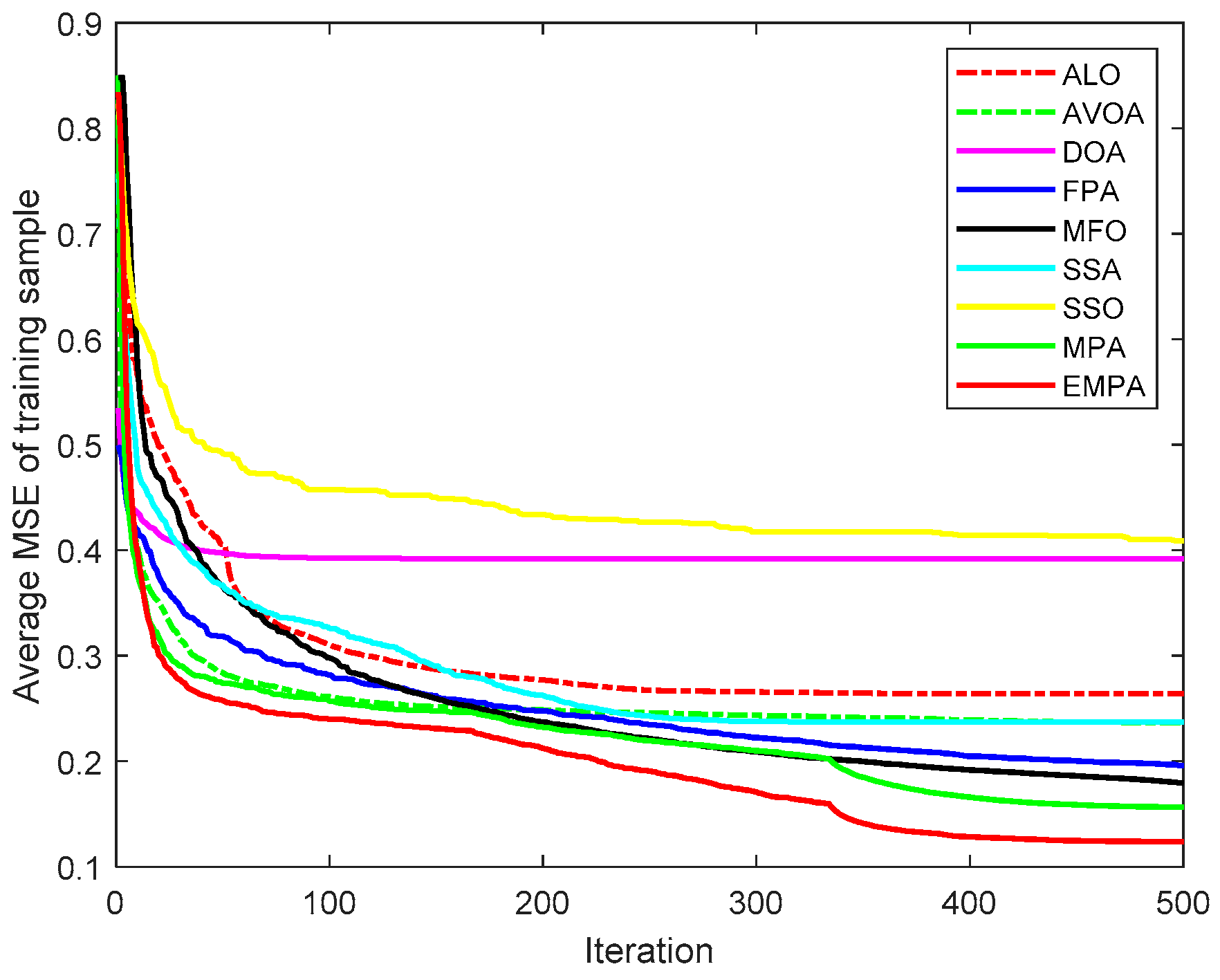
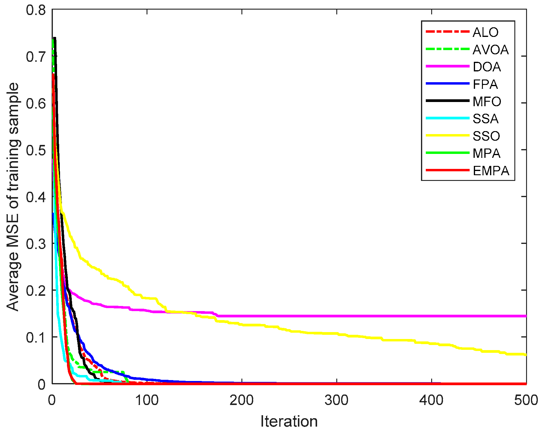
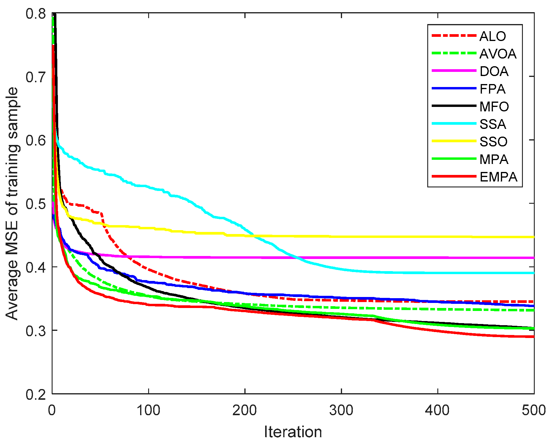
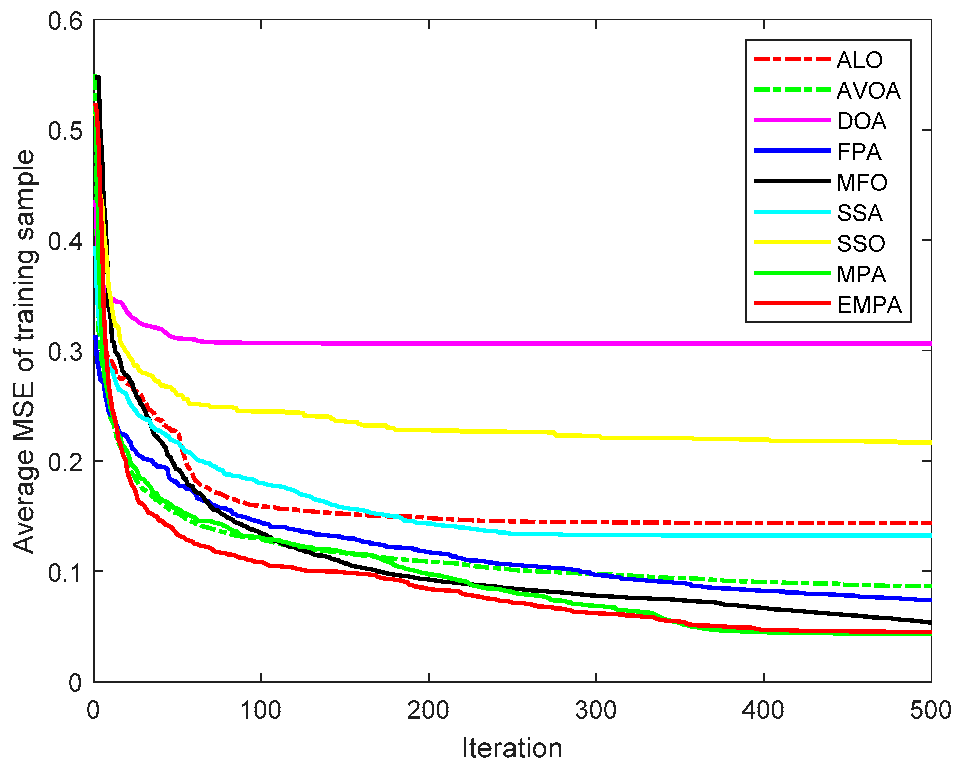
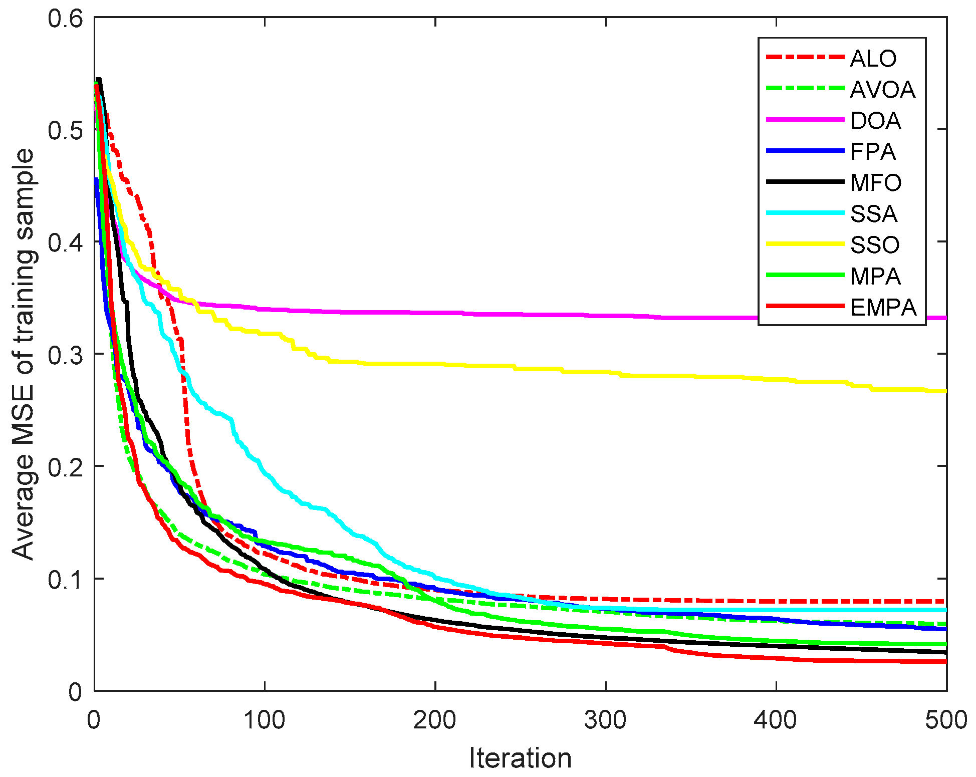
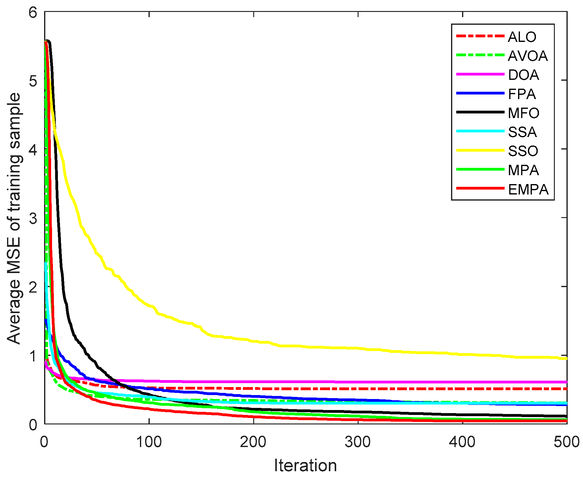
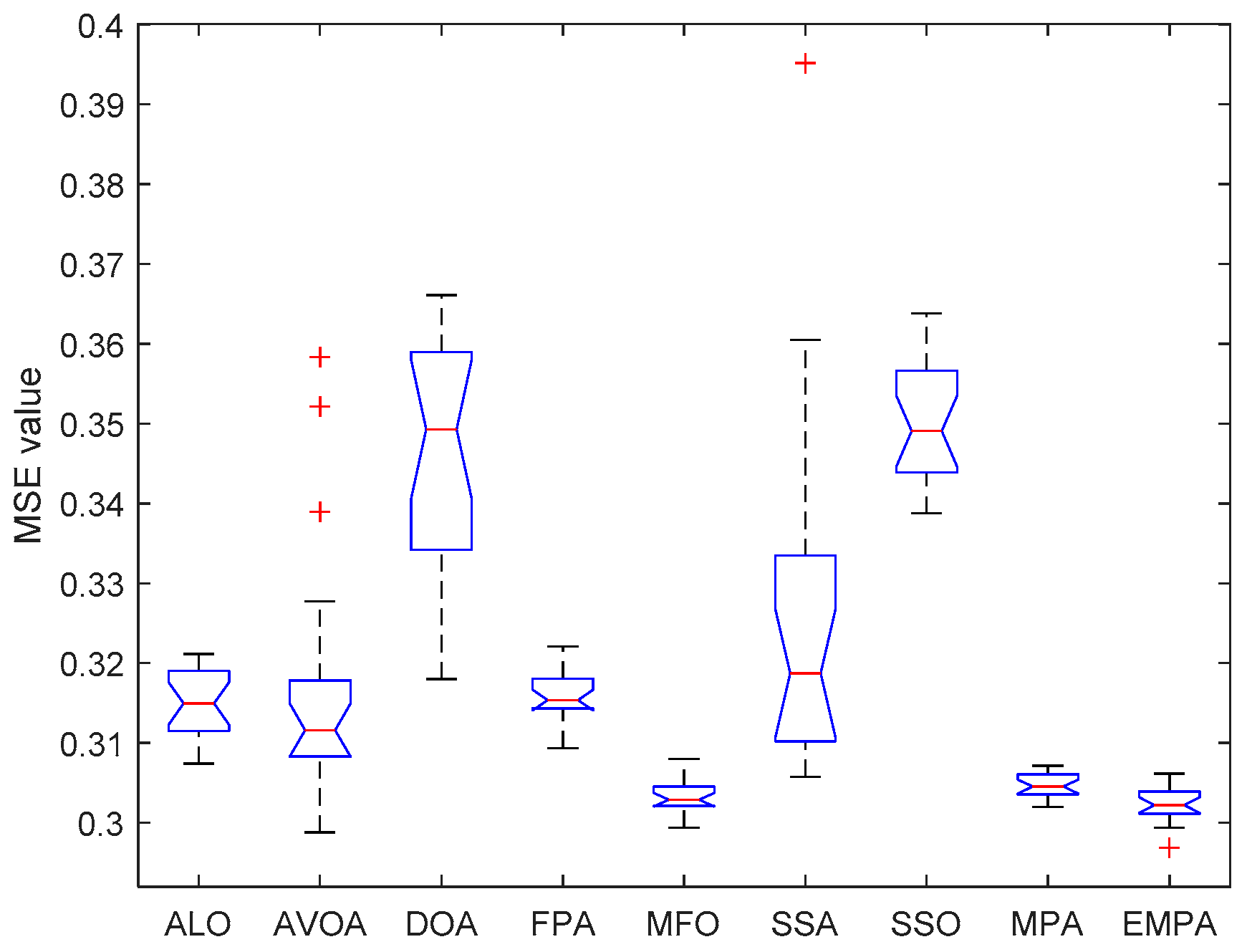
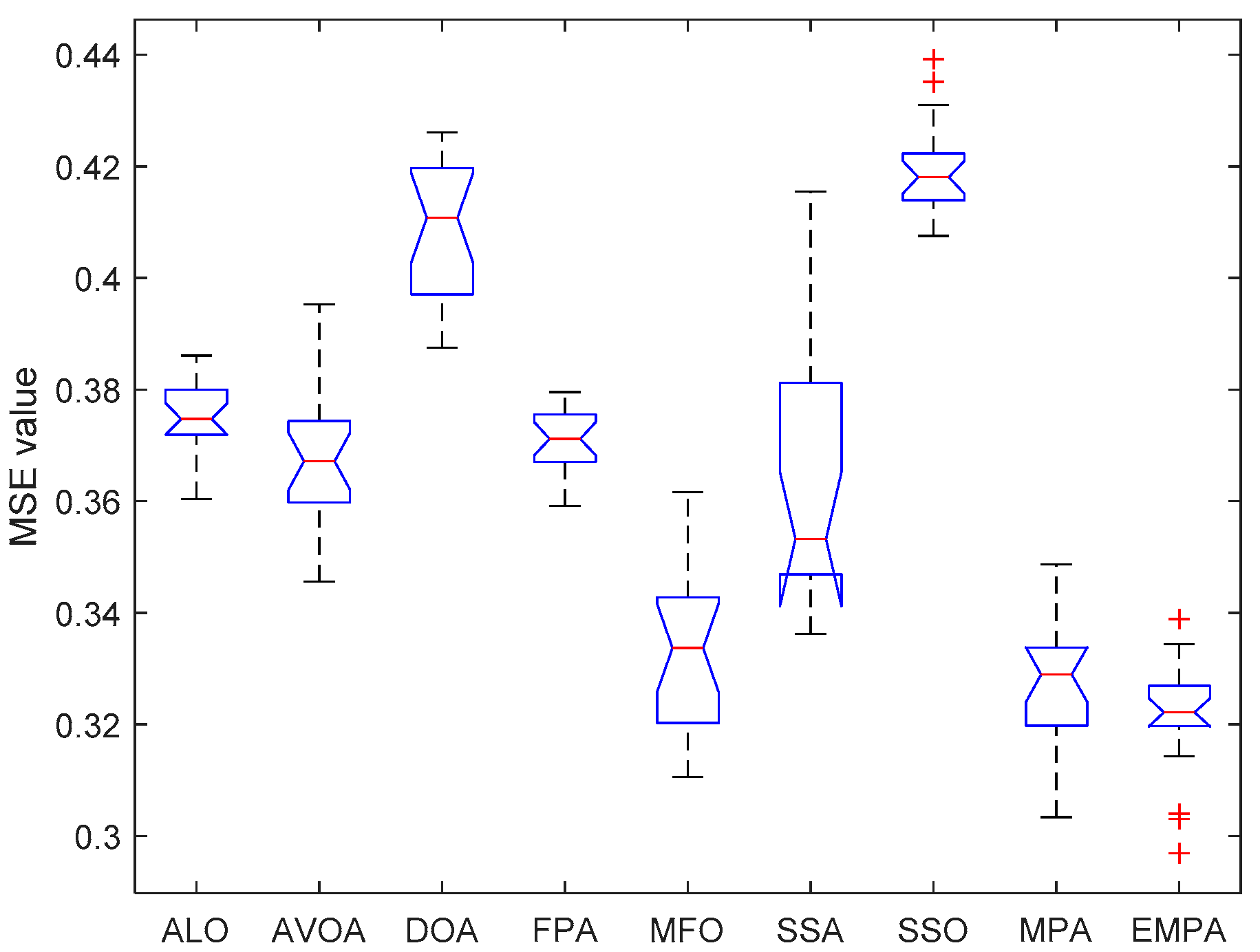
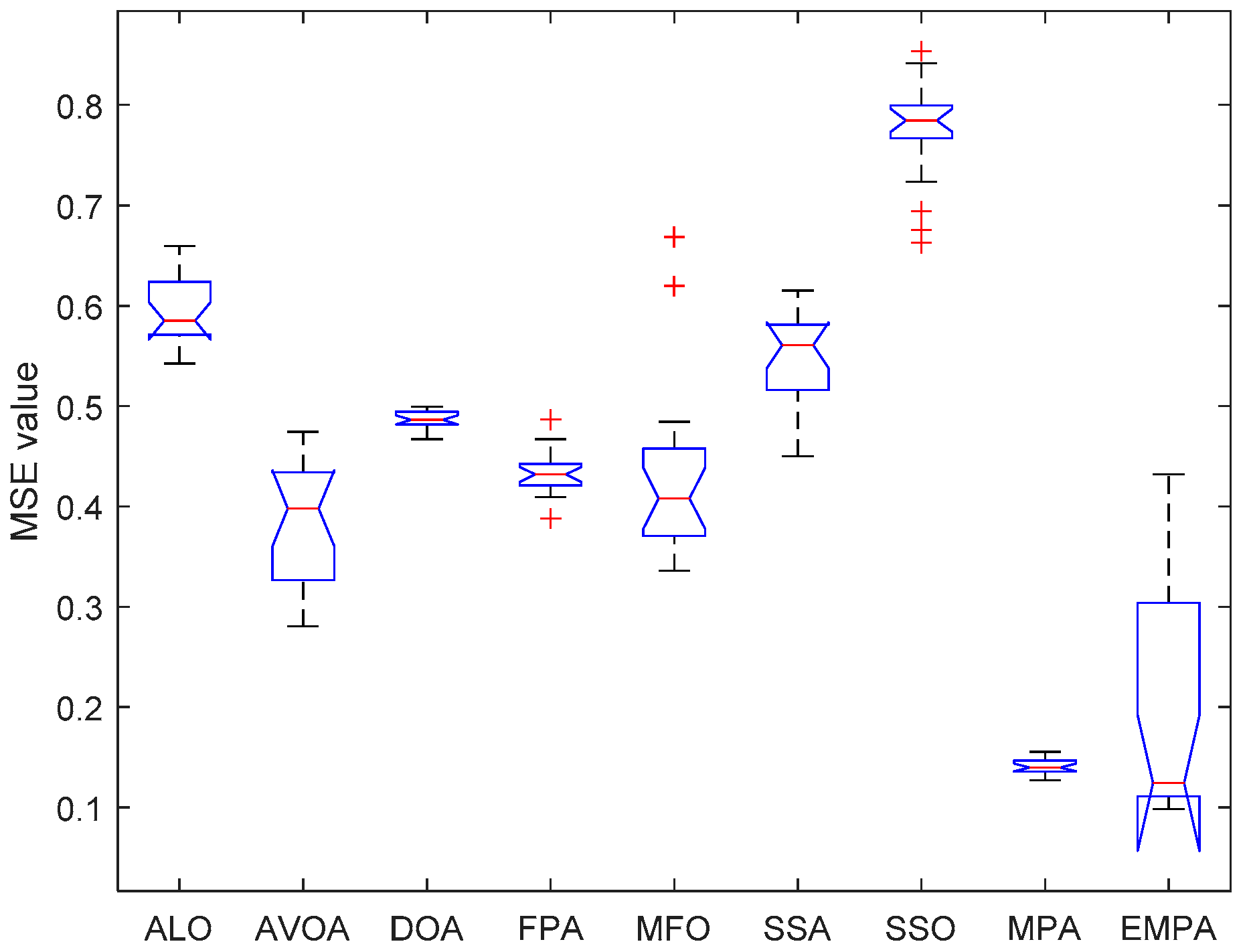
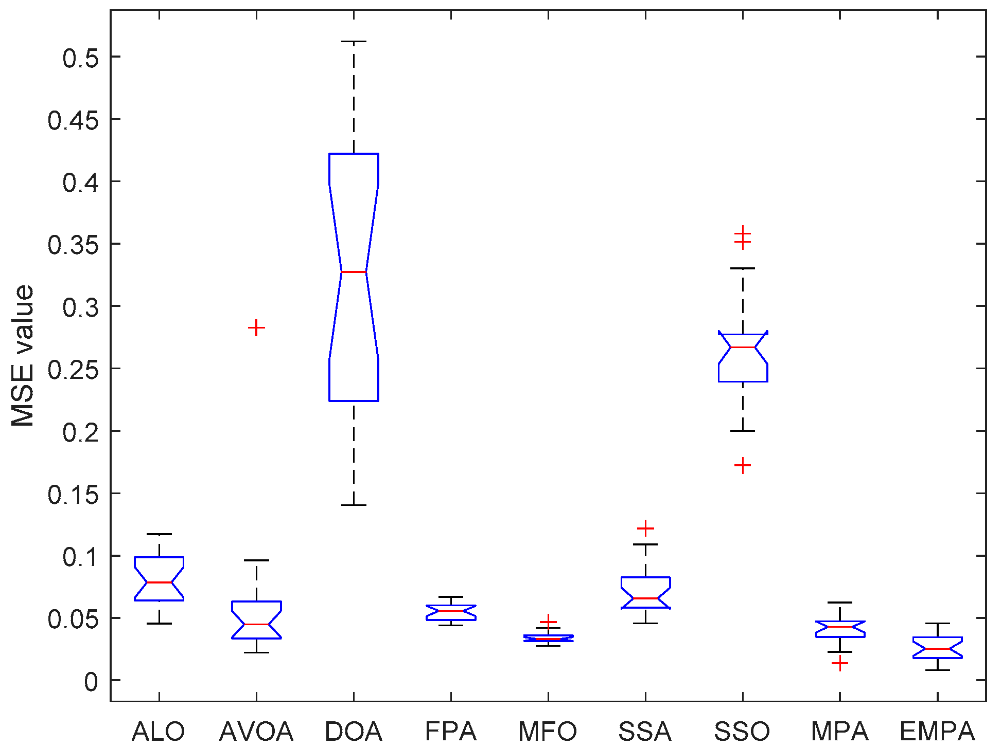
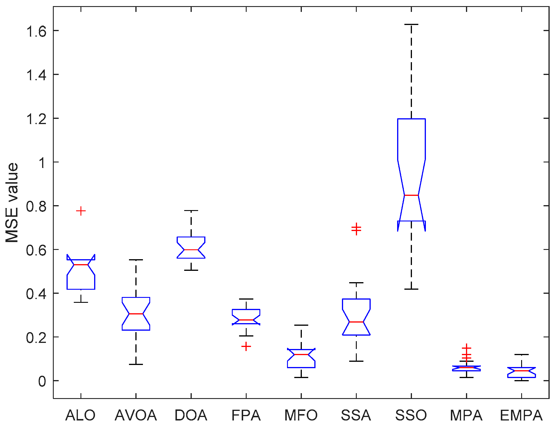
6.4. Results and Analysis
7. Conclusions and Future Research
Author Contributions
Funding
Institutional Review Board Statement
Informed Consent Statement
Data Availability Statement
Acknowledgments
Conflicts of Interest
Abbreviations
| FNNs | Feedforward Neural Networks |
| MPA | Marine Predators Algorithm |
| EMPA | Enhanced Marine Predators Algorithm |
| UCI | University of California Irvine |
| ALO | Ant Lion Optimization |
| AVOA | African Vultures Optimization Algorithm |
| DOA | Dingo Optimization Algorithm |
| FPA | Flower Pollination Algorithm |
| MFO | Moth Flame Optimization |
| SSA | Salp Swarm Algorithm |
| SSO | Sperm Swarm Optimization |
| MLP | Multilayer Perception |
| MSE | Mean Squared Error |
| N/A | Not Applicable |
References
- Üstün, O.; Bekiroğlu, E.; Önder, M. Design of highly effective multilayer feedforward neural network by using genetic algorithm. Expert Syst. 2020, 37, e12532. [Google Scholar] [CrossRef]
- Yin, Y.; Tu, Q.; Chen, X. Enhanced Salp Swarm Algorithm based on random walk and its application to training feedforward neural networks. Soft Comput. 2020, 24, 14791–14807. [Google Scholar] [CrossRef]
- Troumbis, I.A.; Tsekouras, G.E.; Tsimikas, J.; Kalloniatis, C.; Haralambopoulos, D. A Chebyshev polynomial feedforward neural network trained by differential evolution and its application in environmental case studies. Environ. Model. Softw. 2020, 126, 104663. [Google Scholar] [CrossRef]
- Al-Majidi, S.D.; Abbod, M.F.; Al-Raweshidy, H.S. A particle swarm optimisation-trained feedforward neural network for predicting the maximum power point of a photovoltaic array. Eng. Appl. Artif. Intell. 2020, 92, 103688. [Google Scholar] [CrossRef]
- Truong, T.T.; Dinh-Cong, D.; Lee, J.; Nguyen-Thoi, T. An effective deep feedforward neural networks (DFNN) method for damage identification of truss structures using noisy incomplete modal data. J. Build. Eng. 2020, 30, 101244. [Google Scholar] [CrossRef]
- Mirjalili, S. The ant lion optimizer. Adv. Eng. Softw. 2015, 83, 80–98. [Google Scholar] [CrossRef]
- Abdollahzadeh, B.; Gharehchopogh, F.S.; Mirjalili, S. African vultures optimization algorithm: A new nature-inspired metaheuristic algorithm for global optimization problems. Comput. Ind. Eng. 2021, 158, 107408. [Google Scholar] [CrossRef]
- Bairwa, A.K.; Joshi, S.; Singh, D. Dingo optimizer: A nature-inspired metaheuristic approach for engineering problems. Math. Probl. Eng. 2021, 2021, 2571863. [Google Scholar] [CrossRef]
- Yang, X.-S.; Karamanoglu, M.; He, X. Flower pollination algorithm: A novel approach for multiobjective optimization. Eng. Optim. 2014, 46, 1222–1237. [Google Scholar] [CrossRef]
- Mirjalili, S. Moth-flame optimization algorithm: A novel nature-inspired heuristic paradigm. Knowl. Based Syst. 2015, 89, 228–249. [Google Scholar] [CrossRef]
- Mirjalili, S.; Gandomi, A.H.; Mirjalili, S.Z.; Saremi, S.; Faris, H.; Mirjalili, S.M. Salp Swarm Algorithm: A bio-inspired optimizer for engineering design problems. Adv. Eng. Softw. 2017, 114, 163–191. [Google Scholar] [CrossRef]
- Eslami, M.; Babaei, B.; Shareef, H.; Khajehzadeh, M.; Arandian, B. Optimum design of damping controllers using modified Sperm swarm optimization. IEEE Access 2021, 9, 145592–145604. [Google Scholar] [CrossRef]
- Zhang, S.; Xie, L. Grafting constructive algorithm in feedforward neural network learning. Appl. Intell. 2022, 1–18. [Google Scholar] [CrossRef]
- Fan, Y.; Yang, W. A Backpropagation Learning Algorithm with Graph Regularization for Feedforward Neural Networks. Inf. Sci. 2022, 607, 263–277. [Google Scholar] [CrossRef]
- Qu, Z.; Liu, X.; Sun, L. Learnable antinoise-receiver algorithm based on a quantum feedforward neural network in optical quantum communication. Phys. Rev. A 2022, 105, 052427. [Google Scholar] [CrossRef]
- Admon, M.R.; Senu, N.; Ahmadian, A.; Majid, Z.A.; Salahshour, S. A new efficient algorithm based on feedforward neural network for solving differential equations of fractional order. Commun. Nonlinear Sci. Numer. Simul. 2022, 177, 106968. [Google Scholar] [CrossRef]
- Guo, W.; Qiu, H.; Liu, Z.; Zhu, J.; Wang, Q. An integrated model based on feedforward neural network and Taylor expansion for indicator correlation elimination. Intell. Data Anal. 2022, 26, 751–783. [Google Scholar] [CrossRef]
- Zhang, G. Research on safety simulation model and algorithm of dynamic system based on artificial neural network. Soft Comput. 2022, 26, 7377–7386. [Google Scholar] [CrossRef]
- Venkatachalapathy, P.; Mallikarjunaiah, S.M. A feedforward neural network framework for approximating the solutions to nonlinear ordinary differential equations. Neural Comput. Appl. 2022, 35, 1661–1673. [Google Scholar] [CrossRef]
- Liao, G.; Zhang, L. Solving flows of dynamical systems by deep neural networks and a novel deep learning algorithm. Math. Comput. Simul. 2022, 202, 331–342. [Google Scholar] [CrossRef]
- Shao, R.; Zhang, G.; Gong, X. Generalized robust training scheme using genetic algorithm for optical neural networks with imprecise components. Photon. Res. 2022, 10, 1868–1876. [Google Scholar] [CrossRef]
- Wu, C.; Wang, C.; Kim, J.-W. Welding sequence optimization to reduce welding distortion based on coupled artificial neural network and swarm intelligence algorithm. Eng. Appl. Artif. Intell. 2022, 114, 105142. [Google Scholar] [CrossRef]
- Raziani, S.; Ahmadian, S.; Jalali, S.M.J.; Chalechale, A. An Efficient Hybrid Model Based on Modified Whale Optimization Algorithm and Multilayer Perceptron Neural Network for Medical Classification Problems. J. Bionic Eng. 2022, 19, 1504–1521. [Google Scholar] [CrossRef]
- Dong, Z.; Huang, H. A training algorithm with selectable search direction for complex-valued feedforward neural networks. Neural Netw. 2021, 137, 75–84. [Google Scholar] [CrossRef]
- Fontes, C.H.; Embiruçu, M. An approach combining a new weight initialization method and constructive algorithm to configure a single Feedforward Neural Network for multi-class classification. Eng. Appl. Artif. Intell. 2021, 106, 104495. [Google Scholar] [CrossRef]
- Zheng, M.; Luo, J.; Dang, Z. Feedforward neural network based time-varying state-transition-matrix of Tschauner-Hempel equations. Adv. Space Res. 2022, 69, 1000–1011. [Google Scholar] [CrossRef]
- Yılmaz, O.; Bas, E.; Egrioglu, E. The training of Pi-Sigma artificial neural networks with differential evolution algorithm for forecasting. Comput. Econ. 2022, 59, 1699–1711. [Google Scholar] [CrossRef]
- Luo, Q.; Li, J.; Zhou, Y.; Liao, L. Using spotted hyena optimizer for training feedforward neural networks. Cogn. Syst. Res. 2021, 65, 1–16. [Google Scholar] [CrossRef]
- Askari, Q.; Younas, I. Political optimizer based feedforward neural network for classification and function approximation. Neural Process. Lett. 2021, 53, 429–458. [Google Scholar] [CrossRef]
- Duman, S.; Dalcalı, A.; Özbay, H. Manta ray foraging optimization algorithm–based feedforward neural network for electric energy consumption forecasting. Int. Trans. Electr. Energy Syst. 2021, 31, e12999. [Google Scholar] [CrossRef]
- Pan, X.-M.; Song, B.-Y.; Wu, D.; Wei, G.; Sheng, X.-Q. On Phase Information for Deep Neural Networks to Solve Full-Wave Nonlinear Inverse Scattering Problems. IEEE Antennas Wirel. Propag. Lett. 2021, 20, 1903–1907. [Google Scholar] [CrossRef]
- Wu, Q.; Chen, Z.; Chen, D.; Li, S. Beetle antennae search strategy for neural network model optimization with application to glomerular filtration rate estimation. Neural Process. Lett. 2021, 53, 1501–1522. [Google Scholar] [CrossRef]
- Mahmoud, M.A.B.; Guo, P.; Fathy, A.; Li, K. SRCNN-PIL: Side Road Convolution Neural Network Based on Pseudoinverse Learning Algorithm. Neural Process. Lett. 2021, 53, 4225–4237. [Google Scholar] [CrossRef]
- Jamshidi, M.B.; Daneshfar, F. A Hybrid Echo State Network for Hypercomplex Pattern Recognition, Classification, and Big Data Analysis. In Proceedings of the 2022 12th International Conference on Computer and Knowledge Engineering (ICCKE), Mashhad, Iran, 17–18 November 2022; IEEE: Piscataway, NJ, USA; pp. 7–12. [Google Scholar]
- Khalaj, O.; Jamshidi, M.B.; Saebnoori, E.; Masek, B.; Stadler, C.; Svoboda, J. Hybrid machine learning techniques and computational mechanics: Estimating the dynamic behavior of oxide precipitation hardened steel. IEEE Access 2021, 9, 156930–156946. [Google Scholar] [CrossRef]
- Daneshfar, F.; Jamshidi, M.B. An Octonion-Based Nonlinear Echo State Network for Speech Emotion Recognition in Metaverse. SSRN Electron. J. 2022, 4242011. [Google Scholar]
- Elminaam, D.S.A.; Nabil, A.; Ibraheem, S.A.; Houssein, E.H. An efficient marine predators algorithm for feature selection. IEEE Access 2021, 9, 60136–60153. [Google Scholar] [CrossRef]
- Zhang, J.; Li, X.; Tian, J.; Jiang, Y.; Luo, H.; Yin, S. A variational local weighted deep sub-domain adaptation network for remaining useful life prediction facing cross-domain condition. Reliab. Eng. Syst. Saf. 2023, 231, 108986. [Google Scholar] [CrossRef]
- Zhang, J.; Zhang, K.; An, Y.; Luo, H.; Yin, S. An Integrated Multitasking Intelligent Bearing Fault Diagnosis Scheme Based on Representation Learning Under Imbalanced Sample Condition. IEEE Trans. Neural Netw. Learn. Syst. 2023, 1–12. [Google Scholar] [CrossRef]
- Zhang, J.; Li, X.; Tian, J.; Luo, H.; Yin, S. An integrated multi-head dual sparse self-attention network for remaining useful life prediction. Reliab. Eng. Syst. Saf. 2023, 233, 109096. [Google Scholar] [CrossRef]
- Zhang, J.; Tian, J.; Li, M.; Leon, J.I.; Franquelo, L.G.; Luo, H.; Yin, S. A parallel hybrid neural network with integration of spatial and temporal features for remaining useful life prediction in prognostics. IEEE Trans. Instrum. Meas. 2022, 72, 1–12. [Google Scholar] [CrossRef]
- Faramarzi, A.; Heidarinejad, M.; Mirjalili, S.; Gandomi, A.H. Marine Predators Algorithm: A nature-inspired metaheuristic. Expert Syst. Appl. 2020, 152, 113377. [Google Scholar] [CrossRef]
- Yan, Z.; Zhang, J.; Zeng, J.; Tang, J. Nature-inspired approach: An enhanced whale optimization algorithm for global optimization. Math. Comput. Simul. 2021, 185, 17–46. [Google Scholar] [CrossRef]
- Bridge, P.D.; Sawilowsky, S.S. Increasing physicians’ awareness of the impact of statistics on research outcomes: Comparative power of the t-test and Wilcoxon rank-sum test in small samples applied research. J. Clin. Epidemiol. 1999, 52, 229–235. [Google Scholar] [CrossRef] [PubMed]

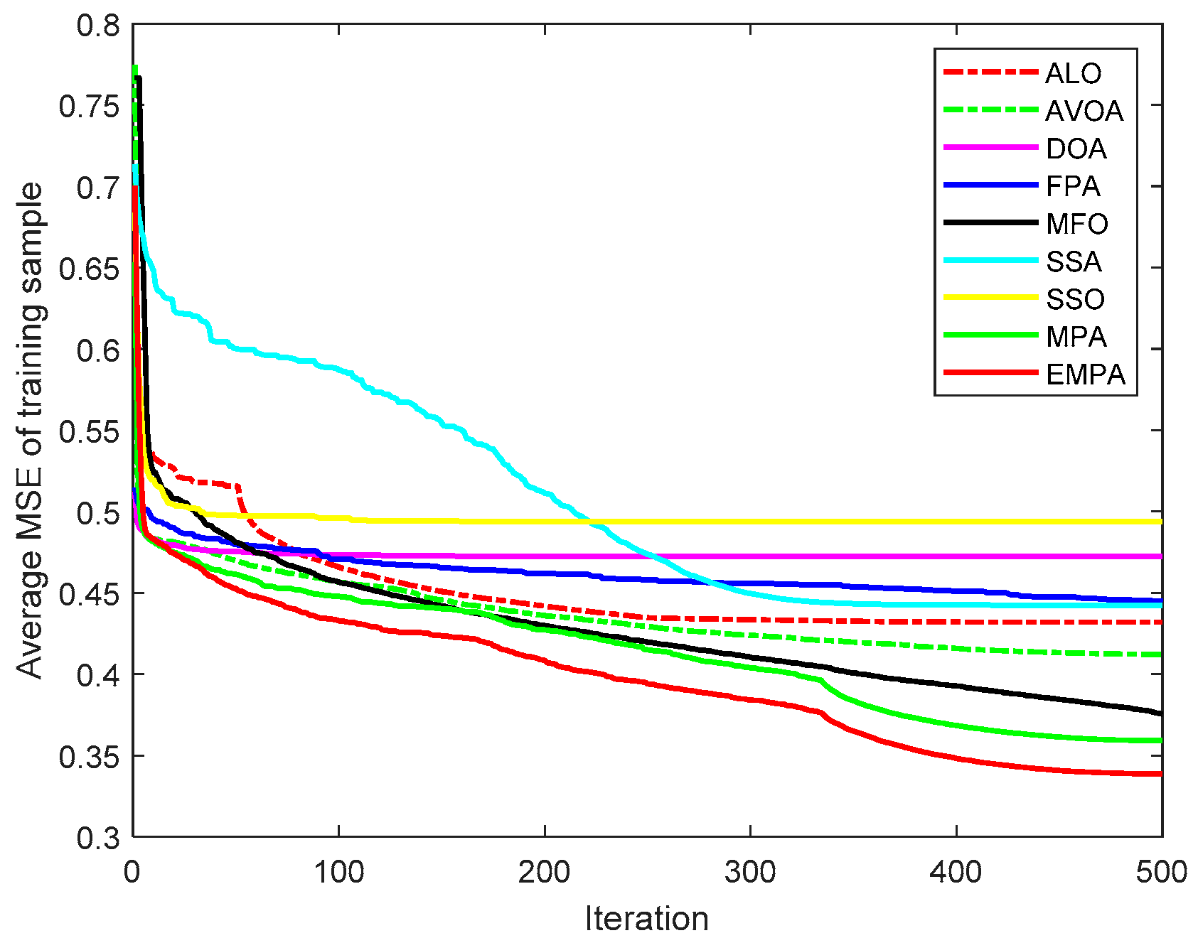
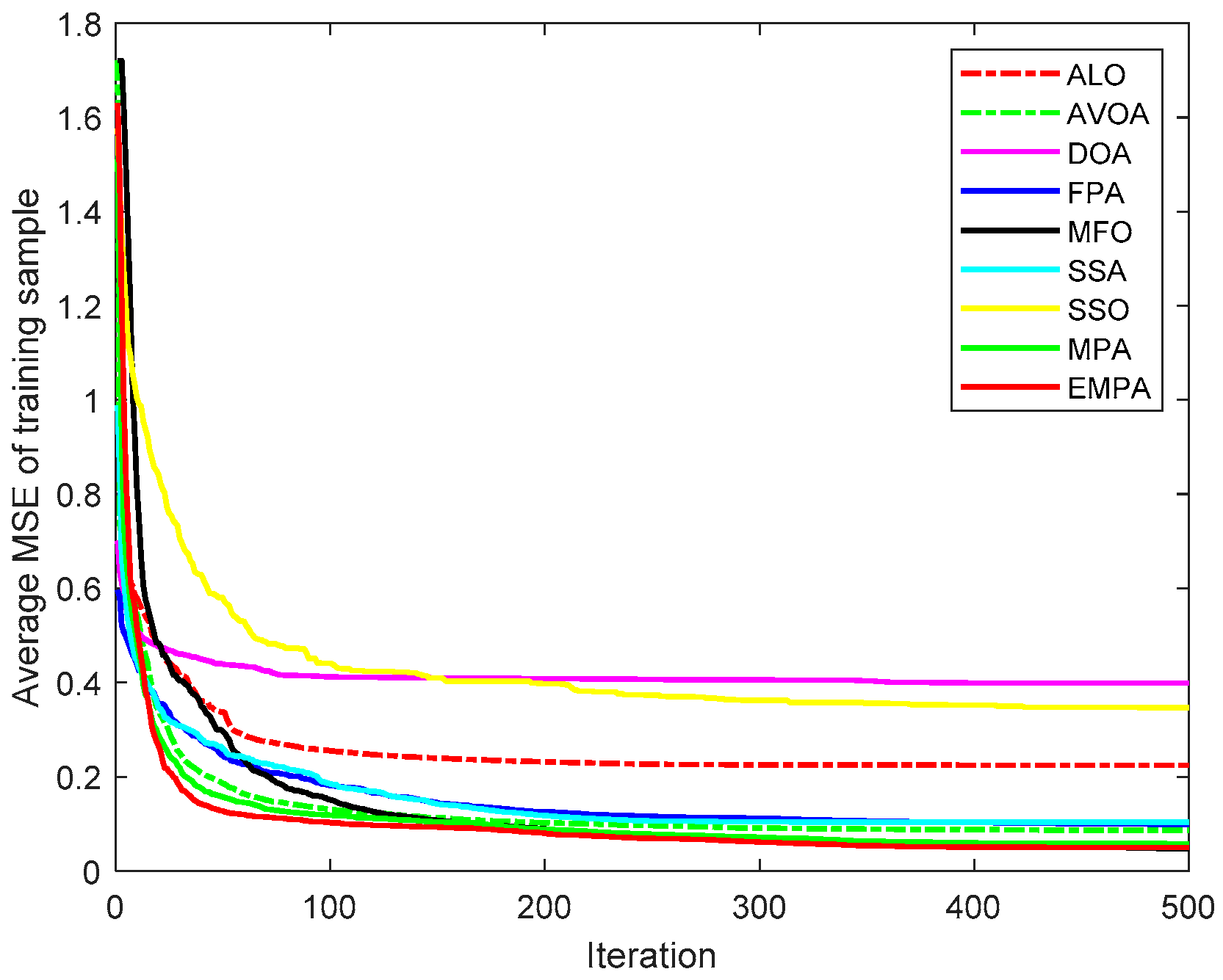
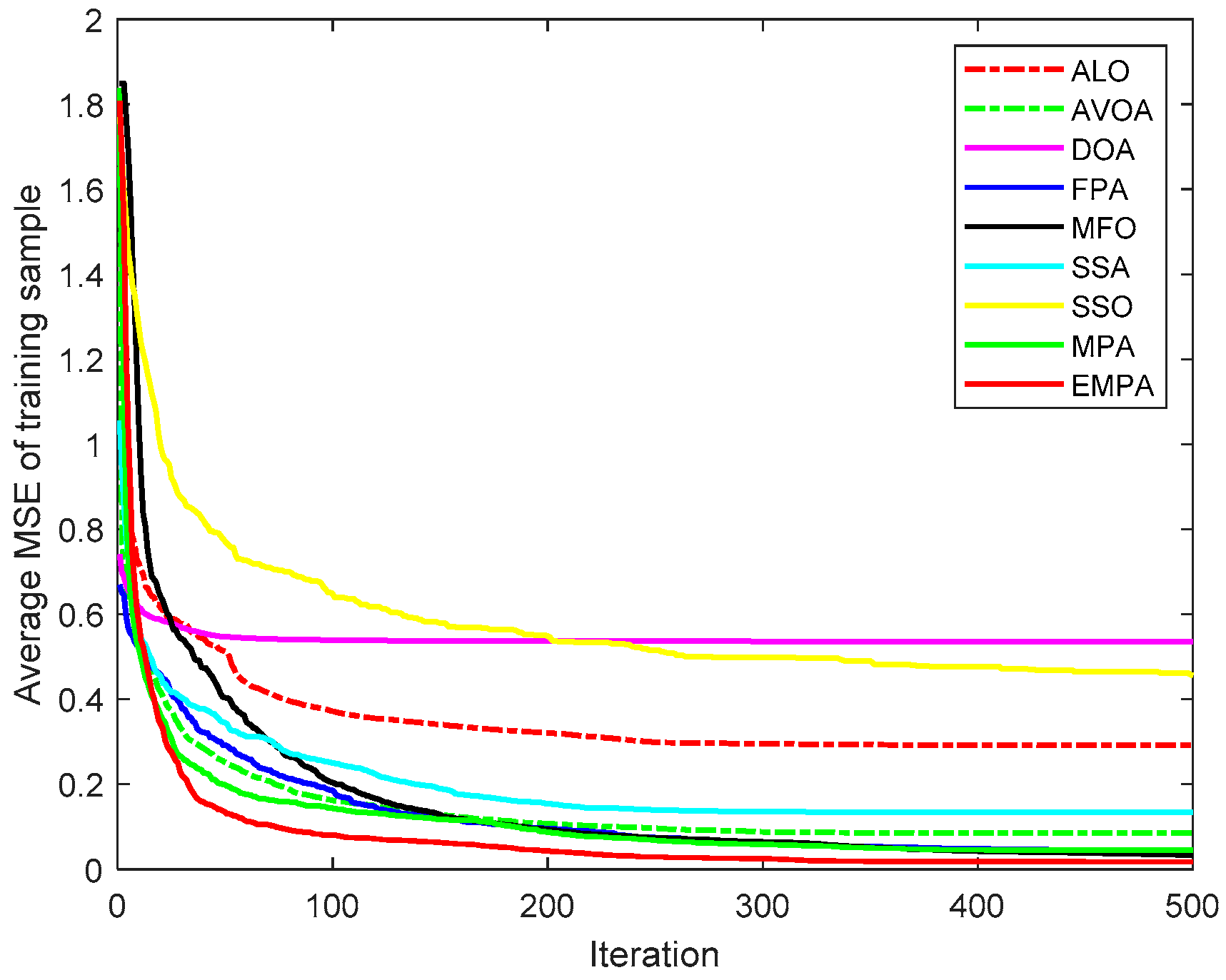
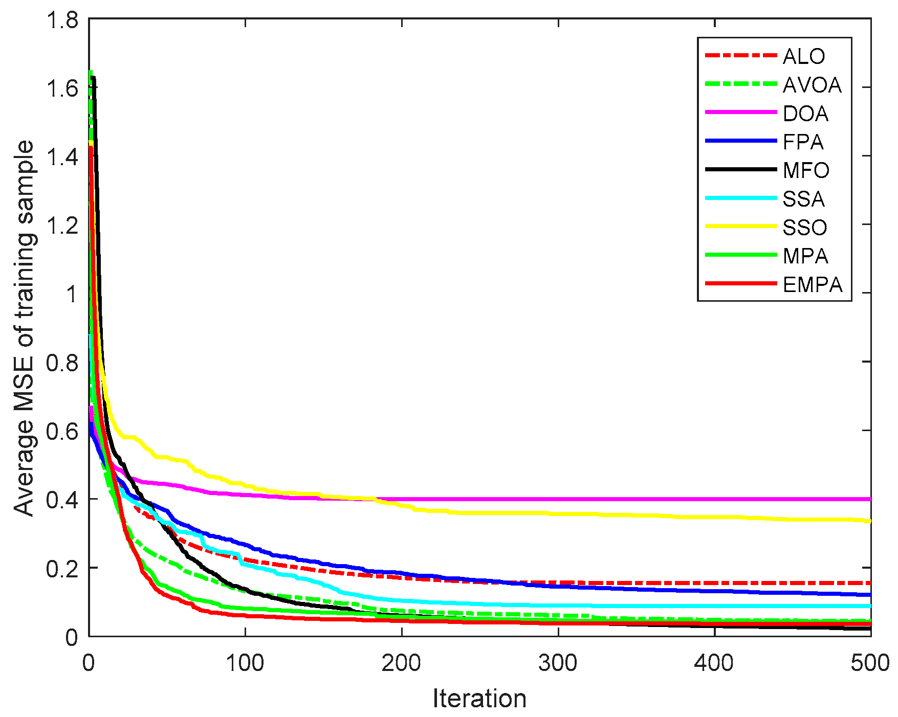





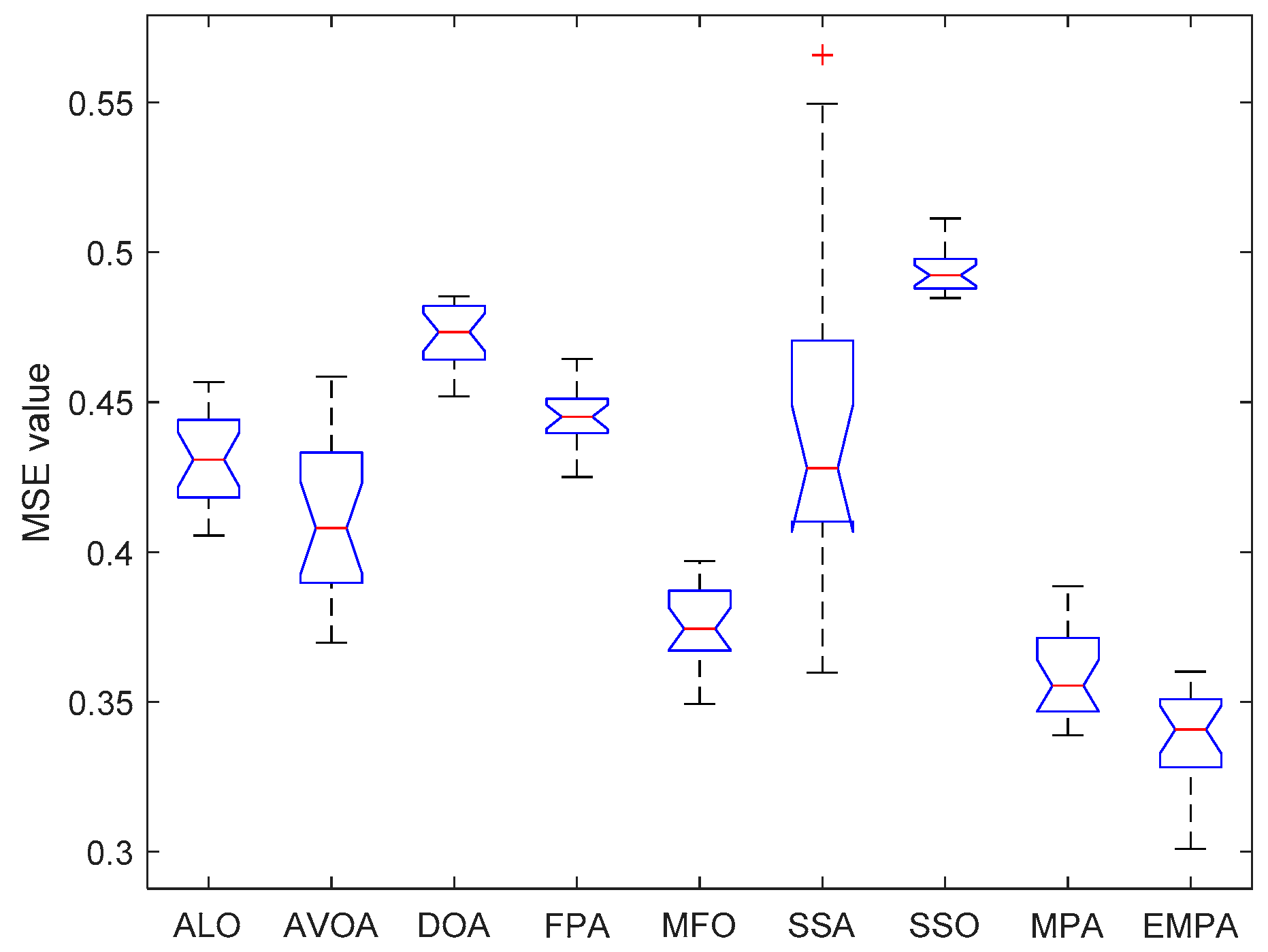
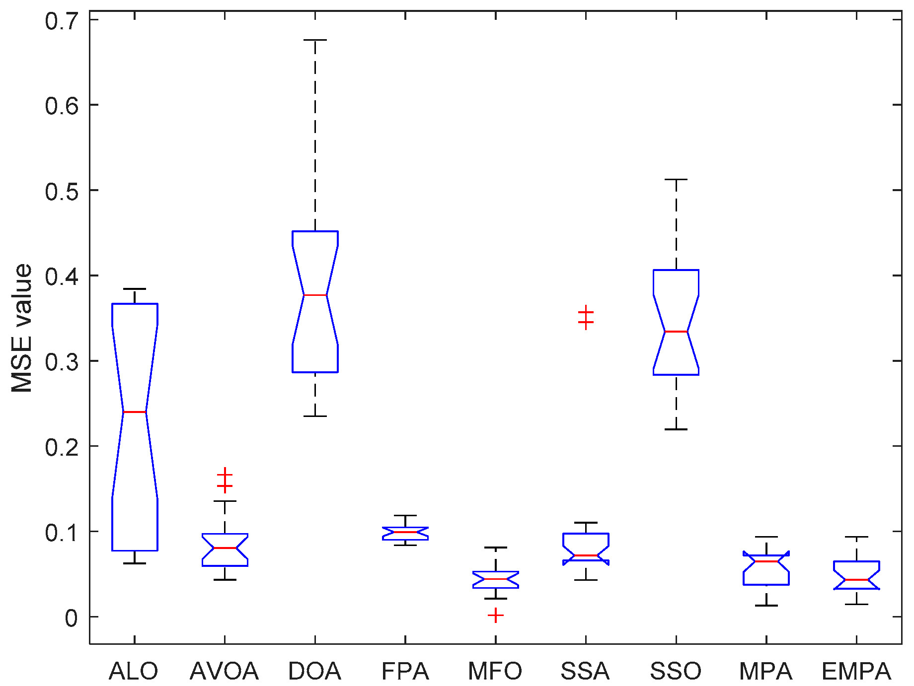
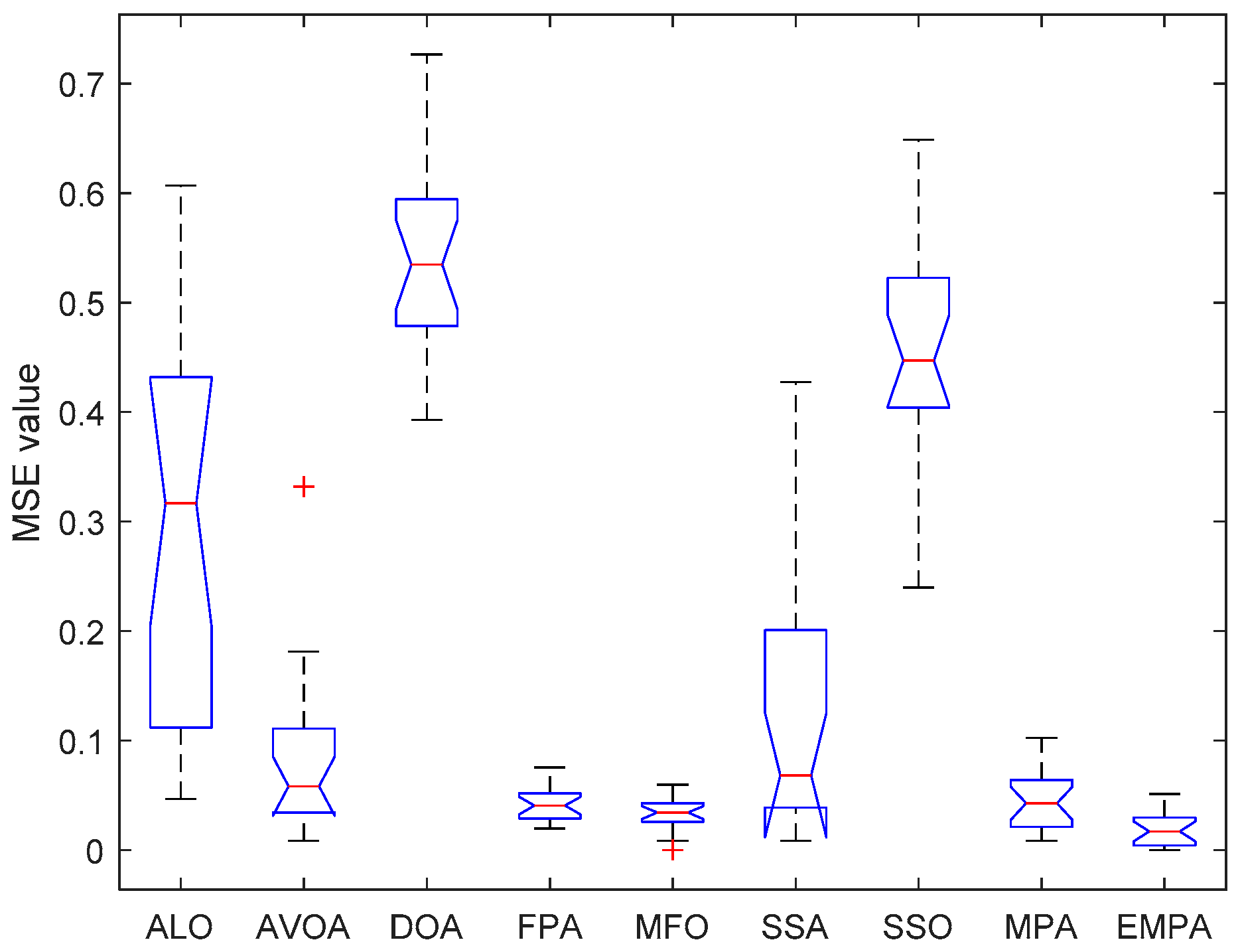
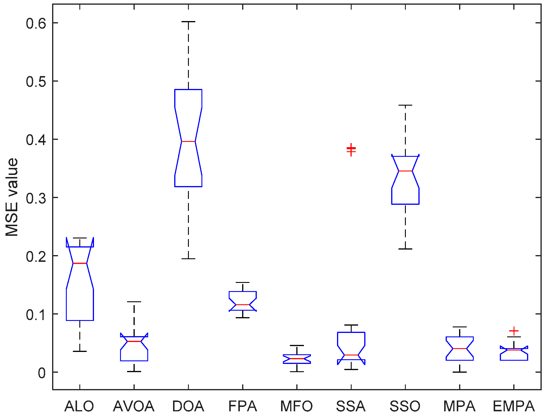
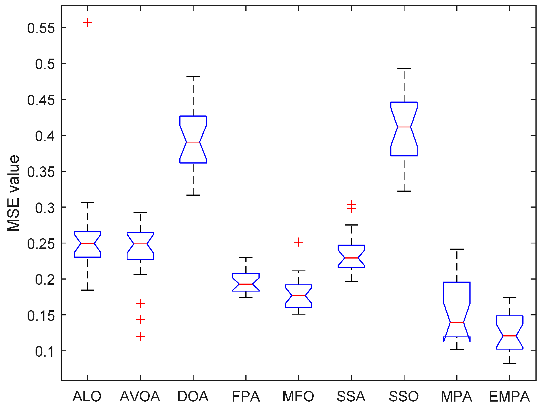
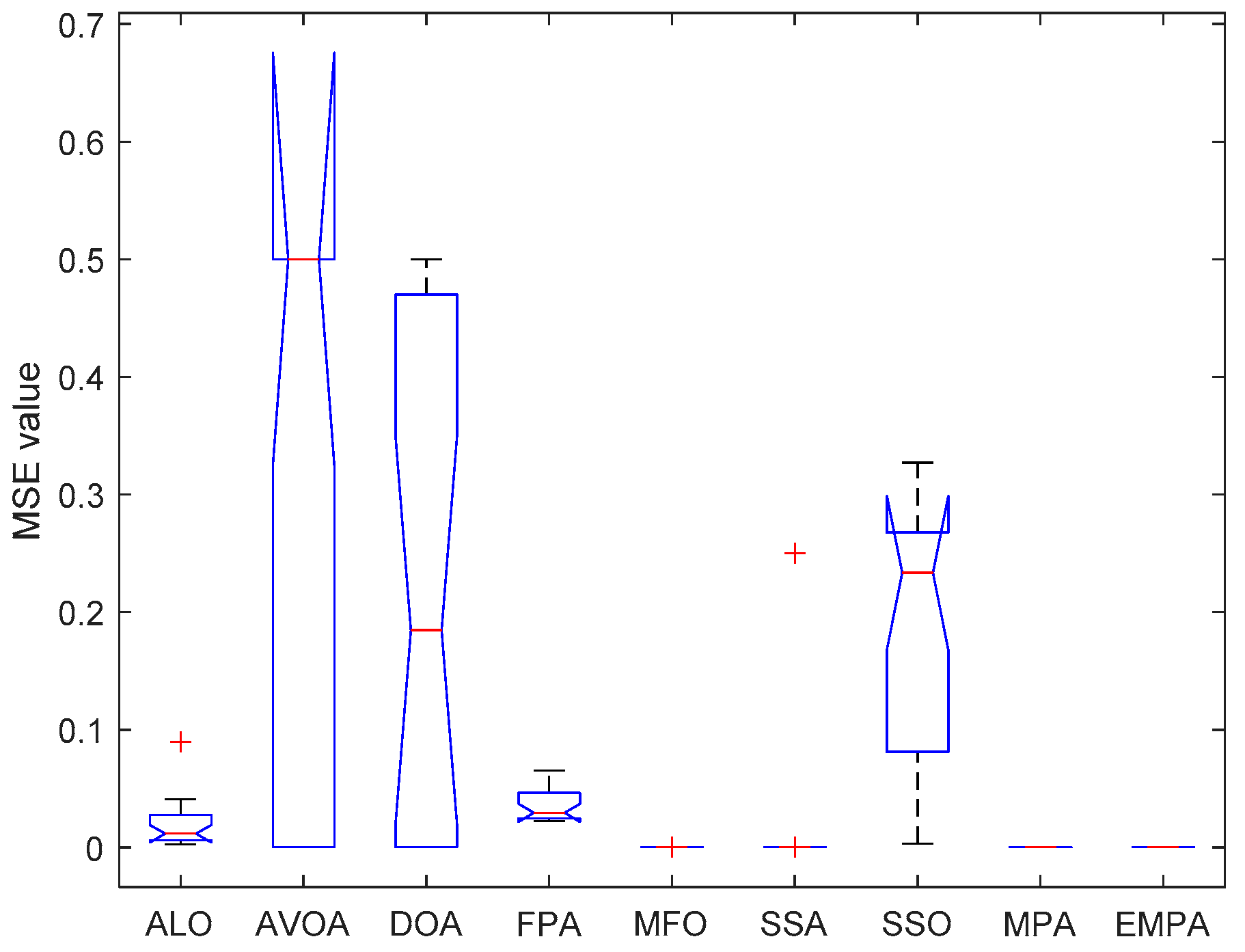


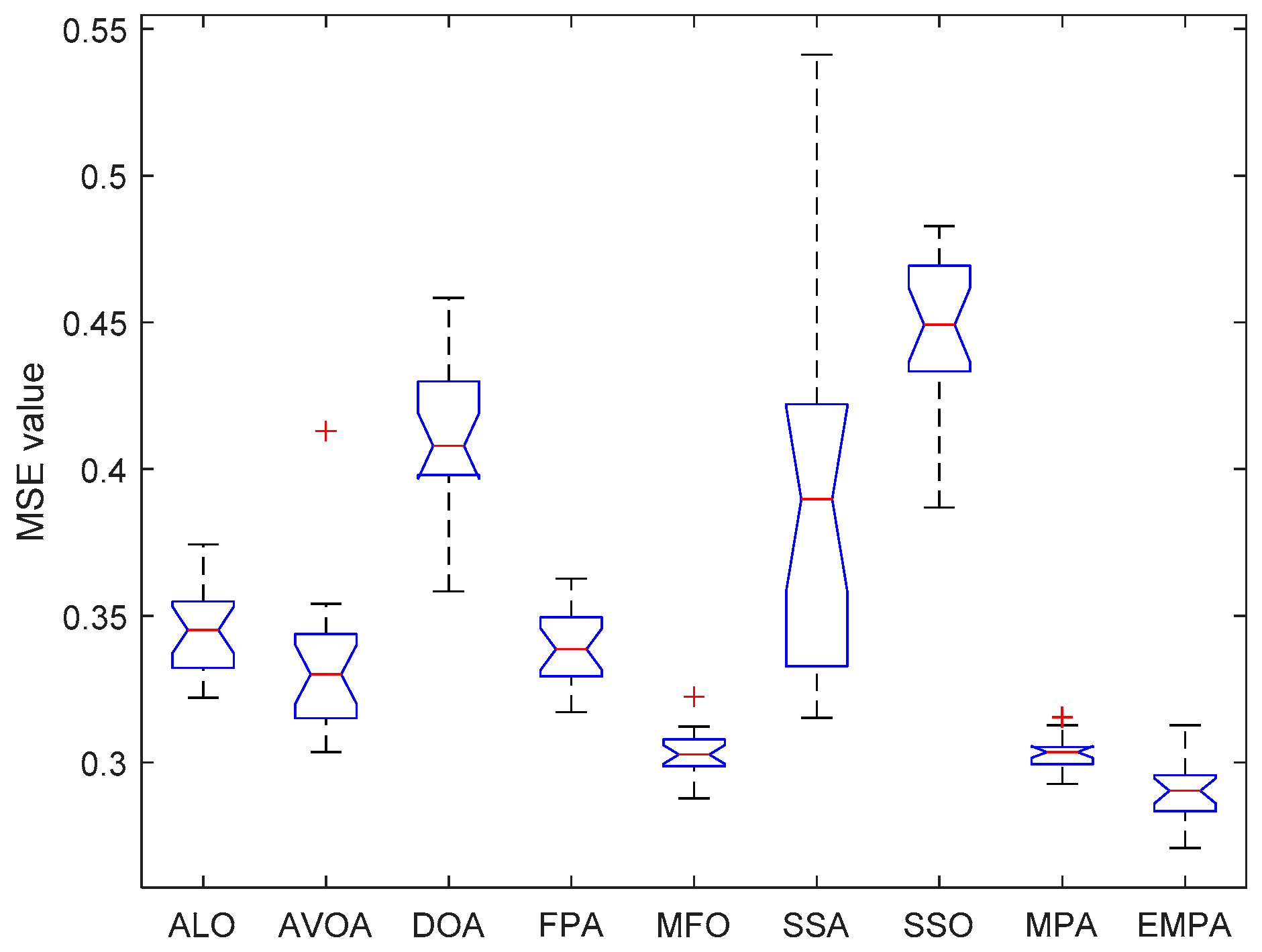
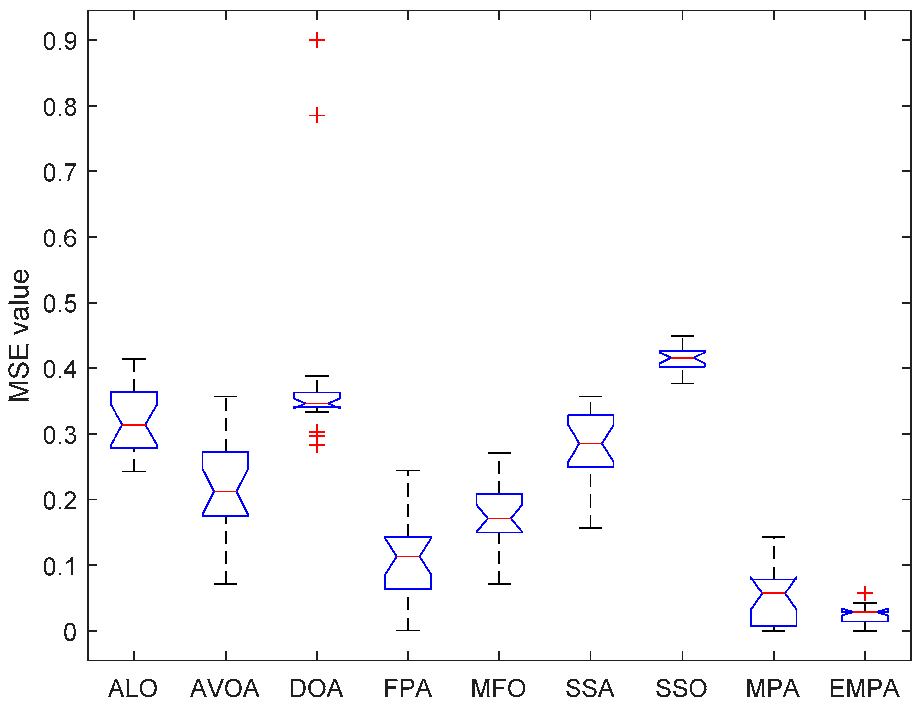

| Issue Scope | EMPA Scope |
|---|---|
| A set scheme to tackle the FNNs | A marine predator population |
| The optimal scheme to obtain the best solution | The marine predator or search agent |
| The evaluation value of FNNs | The fitness value of EMPA |
| Datasets | Attribute | Class | Training | Testing | Input | Hidden | Output |
|---|---|---|---|---|---|---|---|
| Blood | 4 | 2 | 493 | 255 | 4 | 9 | 2 |
| Scale | 4 | 3 | 412 | 213 | 4 | 9 | 3 |
| Survival | 3 | 2 | 202 | 104 | 3 | 7 | 2 |
| Liver | 6 | 2 | 227 | 118 | 6 | 13 | 2 |
| Seeds | 7 | 3 | 139 | 71 | 7 | 15 | 3 |
| Wine | 13 | 3 | 117 | 61 | 13 | 27 | 3 |
| Iris | 4 | 3 | 99 | 51 | 4 | 9 | 3 |
| Statlog | 13 | 2 | 178 | 92 | 13 | 27 | 2 |
| XOR | 3 | 2 | 4 | 4 | 3 | 7 | 2 |
| Balloon | 4 | 2 | 10 | 10 | 4 | 9 | 2 |
| Cancer | 9 | 2 | 599 | 100 | 9 | 19 | 2 |
| Diabetes | 8 | 2 | 507 | 261 | 8 | 17 | 2 |
| Gene | 57 | 2 | 70 | 36 | 57 | 115 | 2 |
| Parkinson | 22 | 2 | 129 | 66 | 22 | 45 | 2 |
| Splice | 60 | 2 | 660 | 340 | 60 | 121 | 2 |
| WDBC | 30 | 2 | 394 | 165 | 30 | 61 | 2 |
| Zoo | 16 | 7 | 67 | 34 | 16 | 33 | 7 |
| Algorithms | Parameters | Values |
|---|---|---|
| ALO | Unpredictable value | [0,1] |
| Constant number | 5 | |
| AVOA | Randomized number | [0,1] |
| Randomized number | [0,1] | |
| Randomized number | [−1,1] | |
| Randomized number | [−2,2] | |
| Randomized number | [0,1] | |
| Randomized number | [0,1] | |
| Randomized number | [0,1] | |
| Constant number | 1.5 | |
| DOA | Randomized vector | [0,1] |
| Randomized vector | [0,1] | |
| Coefficient vector | (1,0) | |
| Coefficient vector | (1,1) | |
| Randomized number | (0,3) | |
| FPA | Switch probability | 0.8 |
| Step size | 1.5 | |
| Randomized number | [0,1] | |
| MFO | Constant number | 1 |
| Randomized number | [−1,1] | |
| Randomized number | [−2,−1] | |
| SSA | Randomized number | [0,1] |
| Randomized number | [0,1] | |
| SSO | Velocity damping factor | [0,1] |
| Randomized number | [7,14] | |
| Randomized number | [7,14] | |
| Randomized number | [7,14] | |
| MPA | Uniform randomized number | [0,1] |
| Uniform randomized number | [0,1] | |
| Constant number | 0.5 | |
| Probability of effect | 0.2 | |
| Binary vector | [0,1] | |
| Randomized number | [0,1] | |
| MPA | Uniform randomized number | [0,1] |
| Uniform randomized number | [0,1] | |
| Constant number | 0.5 | |
| Probability of effect | 0.2 | |
| Binary vector | [0,1] | |
| Randomized number | [0,1] | |
| Scaling factor | 0.7 |
| Datasets | Result | ALO | AVOA | DOA | FPA | MFO | SSA | SSO | MPA | EMPA |
|---|---|---|---|---|---|---|---|---|---|---|
| Blood | Best | 3.07 × 10⁻¹ | 2.99 × 10⁻¹ | 3.18 × 10⁻¹ | 3.09 × 10⁻¹ | 2.99 × 10⁻¹ | 3.06 × 10⁻¹ | 3.39 × 10⁻¹ | 3.02 × 10⁻¹ | 2.96 × 10⁻¹ |
| Worst | 3.21 × 10⁻¹ | 3.58 × 10⁻¹ | 3.66 × 10⁻¹ | 3.22 × 10⁻¹ | 3.08 × 10⁻¹ | 3.95 × 10⁻¹ | 3.64 × 10⁻¹ | 3.07 × 10⁻¹ | 3.06 × 10⁻¹ | |
| Mean | 3.15 × 10⁻¹ | 3.17 × 10⁻¹ | 3.47 × 10⁻¹ | 3.16 × 10⁻¹ | 3.03 × 10⁻¹ | 3.26 × 10⁻¹ | 3.50 × 10⁻¹ | 3.05 × 10⁻¹ | 3.02 × 10⁻¹ | |
| Std | 4.25 × 10⁻³ | 1.55 × 10⁻² | 1.49 × 10⁻² | 2.99 × 10⁻³ | 2.07 × 10⁻³ | 2.21 × 10⁻² | 7.50 × 10⁻³ | 1.53 × 10⁻³ | 2.31 × 10⁻³ | |
| Accuracy | 80.39 | 80.39 | 79.61 | 80 | 80 | 80 | 77.25 | 81.57 | 85.21 | |
| Rank | 3 | 3 | 5 | 4 | 4 | 4 | 6 | 2 | 1 | |
| Scale | Best | 1.39 × 10⁻¹ | 1.21 × 10⁻¹ | 2.86 × 10⁻¹ | 1.56 × 10⁻¹ | 1.20 × 10⁻¹ | 1.28 × 10⁻¹ | 2.27 × 10⁻¹ | 1.05 × 10⁻¹ | 9.74× 10⁻² |
| Worst | 1.86 × 10⁻¹ | 2.99 × 10⁻¹ | 6.42 × 10⁻¹ | 1.85 × 10⁻¹ | 1.57 × 10⁻¹ | 2.13 × 10⁻¹ | 4.79 × 10⁻¹ | 1.79 × 10⁻¹ | 1.57 × 10⁻¹ | |
| Mean | 1.60 × 10⁻¹ | 1.80 × 10⁻¹ | 4.69 × 10⁻¹ | 1.68 × 10⁻¹ | 1.41 × 10⁻¹ | 1.59 × 10⁻¹ | 3.63 × 10⁻¹ | 1.33 × 10⁻¹ | 1.23 × 10⁻¹ | |
| Std | 1.18 × 10⁻² | 5.18 × 10⁻² | 9.35 × 10⁻² | 7.18 × 10⁻³ | 9.75 × 10⁻³ | 2.24 × 10⁻² | 7.96 × 10⁻² | 2.14 × 10⁻² | 1.68 × 10⁻² | |
| Accuracy | 89.20 | 86.85 | 79.34 | 88.03 | 87.32 | 90.14 | 85.92 | 90.61 | 92.02 | |
| Rank | 4 | 7 | 9 | 5 | 6 | 3 | 8 | 2 | 1 | |
| Survival | Best | 3.60 × 10⁻¹ | 3.46 × 10⁻¹ | 3.87 × 10⁻¹ | 3.59 × 10⁻¹ | 3.11 × 10⁻¹ | 3.36 × 10⁻¹ | 4.08 × 10⁻¹ | 3.03 × 10⁻¹ | 2.96 × 10⁻¹ |
| Worst | 3.86 × 10⁻¹ | 3.95 × 10⁻¹ | 4.26 × 10⁻¹ | 3.80 × 10⁻¹ | 3.62 × 10⁻¹ | 4.15 × 10⁻¹ | 4.39 × 10⁻¹ | 3.49 × 10⁻¹ | 3.38 × 10⁻¹ | |
| Mean | 3.75 × 10⁻¹ | 3.67 × 10⁻¹ | 4.09 × 10⁻¹ | 3.71 × 10⁻¹ | 3.33 × 10⁻¹ | 3.64 × 10⁻¹ | 4.19 × 10⁻¹ | 3.27 × 10⁻¹ | 3.21 × 10⁻¹ | |
| Std | 5.74 × 10⁻³ | 1.21 × 10⁻² | 1.30 × 10⁻² | 6.20 × 10⁻³ | 1.46 × 10⁻² | 2.56 × 10⁻² | 8.38 × 10⁻³ | 1.08 × 10⁻² | 1.04 × 10⁻² | |
| Accuracy | 80.76 | 79.33 | 80.29 | 79.81 | 77.88 | 78.85 | 79.33 | 81.73 | 81.94 | |
| Rank | 3 | 6 | 4 | 5 | 8 | 7 | 6 | 2 | 1 | |
| Liver | Best | 4.05 × 10⁻¹ | 3.70 × 10⁻¹ | 4.52 × 10⁻¹ | 4.25 × 10⁻¹ | 3.49 × 10⁻¹ | 3.60 × 10⁻¹ | 4.85 × 10⁻¹ | 3.39 × 10⁻¹ | 3.00 × 10⁻¹ |
| Worst | 4.57 × 10⁻¹ | 4.59 × 10⁻¹ | 4.85 × 10⁻¹ | 4.64 × 10⁻¹ | 3.97 × 10⁻¹ | 5.66 × 10⁻¹ | 5.11 × 10⁻¹ | 3.89 × 10⁻¹ | 3.60 × 10⁻¹ | |
| Mean | 4.32 × 10⁻¹ | 4.12 × 10⁻¹ | 4.72 × 10⁻¹ | 4.45 × 10⁻¹ | 3.76 × 10⁻¹ | 4.42 × 10⁻¹ | 4.94 × 10⁻¹ | 3.59 × 10⁻¹ | 3.38 × 10⁻¹ | |
| Std | 1.54 × 10⁻² | 2.70 × 10⁻² | 1.04 × 10⁻² | 9.28 × 10⁻³ | 1.38 × 10⁻² | 5.63 × 10⁻² | 7.52 × 10⁻³ | 1.47 × 10⁻² | 1.55 × 10⁻² | |
| Accuracy | 69.49 | 71.19 | 56.78 | 60.17 | 72.88 | 60.59 | 56.78 | 74.58 | 75.43 | |
| Rank | 5 | 4 | 8 | 7 | 3 | 6 | 8 | 2 | 1 | |
| Seeds | Best | 6.25 × 10⁻² | 4.32 × 10⁻² | 2.35 × 10⁻¹ | 8.39 × 10⁻² | 1.74 × 10⁻³ | 4.29 × 10⁻² | 2.20 × 10⁻¹ | 1.29 × 10⁻² | 1.43 × 10⁻² |
| Worst | 3.84 × 10⁻¹ | 1.66 × 10⁻¹ | 6.76 × 10⁻¹ | 1.19 × 10⁻¹ | 8.10 × 10⁻² | 3.57 × 10⁻¹ | 5.12 × 10⁻¹ | 9.35 × 10⁻² | 9.35 × 10⁻² | |
| Mean | 2.25 × 10⁻¹ | 8.63 × 10⁻² | 3.99 × 10⁻¹ | 9.85 × 10⁻² | 4.64 × 10⁻² | 1.04 × 10⁻¹ | 3.47 × 10⁻¹ | 5.77 × 10⁻² | 4.94 × 10⁻² | |
| Std | 1.48 × 10⁻¹ | 3.35 × 10⁻² | 1.38 × 10⁻¹ | 8.74 × 10⁻³ | 2.05 × 10⁻² | 8.62 × 10⁻² | 7.81 × 10⁻² | 2.23 × 10⁻² | 2.18 × 10⁻² | |
| Accuracy | 73.38 | 90.14 | 70.42 | 92.96 | 92.96 | 88.73 | 78.87 | 94.37 | 94.43 | |
| Rank | 7 | 4 | 8 | 3 | 3 | 5 | 6 | 2 | 1 | |
| Wine | Best | 4.68 × 10⁻² | 8.55 × 10⁻³ | 3.93 × 10⁻¹ | 1.97 × 10⁻² | 8.68 × 10⁻⁶ | 8.55 × 10⁻³ | 2.39 × 10⁻¹ | 8.54 × 10⁻³ | 0 |
| Worst | 6.07 × 10⁻¹ | 3.32 × 10⁻¹ | 7.26 × 10⁻¹ | 7.55 × 10⁻² | 5.98 × 10⁻² | 4.27 × 10⁻¹ | 6.48 × 10⁻¹ | 1.03 × 10⁻¹ | 5.12 × 10⁻² | |
| Mean | 2.91 × 10⁻¹ | 8.49 × 10⁻² | 5.36 × 10⁻¹ | 4.23 × 10⁻² | 3.28 × 10⁻² | 1.34 × 10⁻¹ | 4.56 × 10⁻¹ | 4.49 × 10⁻² | 1.75 × 10⁻² | |
| Std | 1.62 × 10⁻¹ | 7.77 × 10⁻² | 8.74 × 10⁻² | 1.60 × 10⁻² | 1.56 × 10⁻² | 1.42 × 10⁻¹ | 1.05 × 10⁻¹ | 2.74 × 10⁻² | 1.47 × 10⁻² | |
| Accuracy | 86.89 | 91.80 | 54.10 | 88.52 | 86.88 | 90.16 | 77.05 | 93.44 | 95.08 | |
| Rank | 6 | 3 | 9 | 5 | 7 | 4 | 8 | 2 | 1 | |
| Iris | Best | 3.56× 10⁻² | 9.01× 10⁻⁴ | 1.95 × 10⁻¹ | 9.34× 10⁻² | 6.57× 10⁻⁴ | 4.60× 10⁻³ | 2.12 × 10⁻¹ | 0 | 0 |
| Worst | 2.30 × 10⁻¹ | 1.21 × 10⁻¹ | 6.02 × 10⁻¹ | 1.54 × 10⁻¹ | 4.56× 10⁻² | 3.85 × 10⁻¹ | 4.58 × 10⁻¹ | 7.77× 10⁻² | 7.07× 10⁻² | |
| Mean | 1.55 × 10⁻¹ | 4.55× 10⁻² | 3.99 × 10⁻¹ | 1.21 × 10⁻¹ | 2.23× 10⁻² | 8.86× 10⁻² | 3.35 × 10⁻¹ | 4.27× 10⁻² | 3.64× 10⁻² | |
| Std | 6.72× 10⁻² | 3.16× 10⁻² | 1.20 × 10⁻¹ | 1.98× 10⁻² | 1.15× 10⁻² | 1.28 × 10⁻¹ | 6.16× 10⁻² | 2.20× 10⁻² | 1.48× 10⁻² | |
| Accuracy | 89.22 | 85.29 | 90.20 | 97.55 | 88.24 | 90.20 | 90.20 | 98.04 | 98.23 | |
| Rank | 5 | 7 | 4 | 3 | 6 | 4 | 4 | 2 | 1 | |
| Statlog | Best | 1.85 × 10⁻¹ | 1.20 × 10⁻¹ | 3.17 × 10⁻¹ | 1.74 × 10⁻¹ | 1.51 × 10⁻¹ | 1.97 × 10⁻¹ | 3.22 × 10⁻¹ | 1.02 × 10⁻¹ | 8.25× 10⁻² |
| Worst | 5.57 × 10⁻¹ | 2.92 × 10⁻¹ | 4.81 × 10⁻¹ | 2.30 × 10⁻¹ | 2.51 × 10⁻¹ | 3.03 × 10⁻¹ | 4.93 × 10⁻¹ | 2.42 × 10⁻¹ | 1.74 × 10⁻¹ | |
| Mean | 2.64 × 10⁻¹ | 2.36 × 10⁻¹ | 3.92 × 10⁻¹ | 1.96 × 10⁻¹ | 1.79 × 10⁻¹ | 2.37 × 10⁻¹ | 4.09 × 10⁻¹ | 1.56 × 10⁻¹ | 1.23 × 10⁻¹ | |
| Std | 7.46 × 10⁻² | 4.60 × 10⁻² | 4.52 × 10⁻² | 1.57 × 10⁻² | 2.41 × 10⁻² | 2.90 × 10⁻² | 5.01 × 10⁻² | 4.32 × 10⁻² | 2.68 × 10⁻² | |
| Accuracy | 81.52 | 80.43 | 67.39 | 80.43 | 83.70 | 80.43 | 75 | 85.87 | 85.96 | |
| Rank | 4 | 5 | 7 | 5 | 3 | 5 | 6 | 2 | 1 | |
| XOR | Best | 2.53× 10⁻³ | 0 | 0 | 2.21× 10⁻² | 0 | 1.77 × 10−56 | 3.04 × 10⁻³ | 0 | 0 |
| Worst | 8.96 × 10⁻² | 5.00 × 10⁻¹ | 5.00 × 10⁻¹ | 6.51 × 10⁻² | 4.58 × 10⁻¹¹ | 2.50 × 10⁻¹ | 3.27 × 10⁻¹ | 0 | 0 | |
| Mean | 1.90 × 10⁻² | 3.00 × 10⁻¹ | 2.24 × 10⁻¹ | 3.49 × 10⁻² | 2.30 × 10⁻¹² | 1.25 × 10⁻² | 1.87 × 10⁻¹ | 0 | 0 | |
| Std | 2.01 × 10⁻² | 2.51 × 10⁻¹ | 2.19 × 10⁻¹ | 1.28 × 10⁻² | 1.02 × 10⁻¹¹ | 5.59 × 10⁻² | 1.08 × 10⁻¹ | 0 | 0 | |
| Accuracy | 100 | 50 | 75 | 75 | 50 | 75 | 50 | 100 | 100 | |
| Rank | 1 | 3 | 2 | 2 | 3 | 2 | 3 | 1 | 1 | |
| Balloon | Best | 1.37 × 10⁻⁹ | 0 | 0 | 1.83× 10⁻⁵ | 0 | 0 | 1.82× 10⁻⁴ | 0 | 0 |
| Worst | 9.06 × 10⁻⁵ | 0 | 4.96 × 10⁻¹ | 9.38× 10⁻⁴ | 0 | 5.06 × 10⁻³⁰ | 2.13 × 10⁻¹ | 0 | 0 | |
| Mean | 2.36 × 10⁻⁵ | 0 | 1.45 × 10⁻¹ | 2.23× 10⁻⁴ | 0 | 2.54 × 10⁻³¹ | 6.22 × 10⁻² | 0 | 0 | |
| Std | 3.12 × 10⁻⁵ | 0 | 1.56 × 10⁻¹ | 2.49× 10⁻⁴ | 0 | 1.13 × 10⁻³⁰ | 6.55 × 10⁻² | 0 | 0 | |
| Accuracy | 100 | 100 | 80 | 100 | 80 | 80 | 100 | 100 | 100 | |
| Rank | 1 | 1 | 2 | 1 | 2 | 2 | 1 | 1 | 1 | |
| Cancer | Best | 3.59 × 10⁻² | 3.35 × 10⁻² | 5.92 × 10⁻² | 3.44 × 10⁻² | 2.43 × 10⁻² | 3.69 × 10⁻² | 7.07 × 10⁻² | 2.44 × 10⁻² | 2.15 × 10⁻² |
| Worst | 2.55 × 10⁻¹ | 7.77 × 10⁻² | 2.91 × 10⁻¹ | 4.82 × 10⁻² | 4.84 × 10⁻² | 5.80 × 10⁻² | 1.58 × 10⁻¹ | 5.01 × 10⁻² | 4.50 × 10⁻² | |
| Mean | 7.66 × 10⁻² | 4.78 × 10⁻² | 2.22 × 10⁻¹ | 4.41 × 10⁻² | 3.70 × 10⁻² | 4.62 × 10⁻² | 1.15 × 10⁻¹ | 3.84 × 10⁻² | 3.45 × 10⁻² | |
| Std | 7.31 × 10⁻² | 9.00 × 10⁻³ | 7.57 × 10⁻² | 3.59 × 10⁻³ | 5.19 × 10⁻³ | 5.51 × 10⁻³ | 2.60 × 10⁻² | 6.08 × 10⁻³ | 7.04 × 10⁻³ | |
| Accuracy | 99 | 99 | 98 | 99 | 99 | 99 | 99 | 99 | 99 | |
| Rank | 1 | 1 | 2 | 1 | 1 | 1 | 1 | 1 | 1 | |
| Diabetes | Best | 3.22 × 10⁻¹ | 3.03 × 10⁻¹ | 3.58 × 10⁻¹ | 3.17 × 10⁻¹ | 2.88 × 10⁻¹ | 3.15 × 10⁻¹ | 3.87 × 10⁻¹ | 2.93 × 10⁻¹ | 2.70 × 10⁻¹ |
| Worst | 3.74 × 10⁻¹ | 4.13 × 10⁻¹ | 4.58 × 10⁻¹ | 3.63 × 10⁻¹ | 3.22 × 10⁻¹ | 5.41 × 10⁻¹ | 4.83 × 10⁻¹ | 3.15 × 10⁻¹ | 3.12 × 10⁻¹ | |
| Mean | 3.45 × 10⁻¹ | 3.32 × 10⁻¹ | 4.14 × 10⁻¹ | 3.38 × 10⁻¹ | 3.03 × 10⁻¹ | 3.90 × 10⁻¹ | 4.47 × 10⁻¹ | 3.03 × 10⁻¹ | 2.90 × 10⁻¹ | |
| Std | 1.53 × 10⁻² | 2.48 × 10⁻² | 2.64 × 10⁻² | 1.33 × 10⁻² | 7.50 × 10⁻³ | 6.06 × 10⁻² | 2.76 × 10⁻² | 5.61 × 10⁻³ | 9.99 × 10⁻³ | |
| Accuracy | 78.16 | 77.01 | 74.33 | 80.08 | 77.78 | 78.93 | 67.82 | 80.84 | 80.93 | |
| Rank | 5 | 7 | 8 | 3 | 6 | 4 | 9 | 2 | 1 | |
| Gene | Best | 2.43 × 10⁻¹ | 7.14 × 10⁻² | 2.83 × 10⁻¹ | 5.08 × 10⁻⁴ | 7.14 × 10⁻² | 1.57 × 10⁻¹ | 3.77 × 10⁻¹ | 7.95 × 10⁻¹¹ | 0 |
| Worst | 4.14 × 10⁻¹ | 3.57 × 10⁻¹ | 9.00 × 10⁻¹ | 2.45 × 10⁻¹ | 2.71 × 10⁻¹ | 3.57 × 10⁻¹ | 4.50 × 10⁻¹ | 1.43 × 10⁻¹ | 5.71 × 10⁻² | |
| Mean | 3.19 × 10⁻¹ | 2.18 × 10⁻¹ | 3.93 × 10⁻¹ | 1.08 × 10⁻¹ | 1.78 × 10⁻¹ | 2.79 × 10⁻¹ | 4.15 × 10⁻¹ | 5.22 × 10⁻² | 2.35 × 10⁻² | |
| Std | 5.53 × 10⁻² | 7.55 × 10⁻² | 1.57 × 10⁻¹ | 5.97 × 10⁻² | 5.22× 10⁻² | 5.78 × 10⁻² | 1.86 × 10⁻² | 4.38 × 10⁻² | 1.75 × 10⁻² | |
| Accuracy | 5.56 | 19.44 | 8.33 | 30.56 | 25 | 8.33 | 2.78 | 33.33 | 40.33 | |
| Rank | 7 | 5 | 6 | 3 | 4 | 6 | 8 | 2 | 1 | |
| Parkinson | Best | 7.38 × 10⁻² | 1.99 × 10⁻² | 1.44 × 10⁻¹ | 3.87 × 10⁻² | 4.60 × 10⁻³ | 3.88 × 10⁻² | 1.47 × 10⁻¹ | 1.8 × 10−121 | 0 |
| Worst | 2.33 × 10⁻¹ | 2.56 × 10⁻¹ | 4.04 × 10⁻¹ | 9.76 × 10⁻² | 1.86 × 10⁻¹ | 2.33 × 10⁻¹ | 2.96 × 10⁻¹ | 9.30 × 10⁻² | 9.30 × 10⁻² | |
| Mean | 1.44 × 10⁻¹ | 8.66 × 10⁻² | 3.06 × 10⁻¹ | 7.40 × 10⁻² | 5.36 × 10⁻² | 1.33 × 10⁻¹ | 2.17 × 10⁻¹ | 4.35 × 10⁻² | 4.50 × 10⁻² | |
| Std | 5.42 × 10⁻² | 6.39 × 10⁻² | 7.75 × 10⁻² | 1.71 × 10⁻² | 4.33 × 10⁻² | 6.27 × 10⁻² | 3.69 × 10⁻² | 3.88 × 10⁻² | 3.11 × 10⁻² | |
| Accuracy | 71.21 | 72.73 | 68.18 | 72.73 | 71.21 | 72.73 | 69.70 | 75.76 | 75.76 | |
| Rank | 3 | 2 | 5 | 2 | 3 | 2 | 4 | 1 | 1 | |
| Splice | Best | 5.42 × 10⁻¹ | 2.80 × 10⁻¹ | 4.67 × 10⁻¹ | 3.88 × 10⁻¹ | 3.36 × 10⁻¹ | 4.50 × 10⁻¹ | 6.63 × 10⁻¹ | 1.27 × 10⁻¹ | 9.81 × 10⁻² |
| Worst | 6.59 × 10⁻¹ | 4.74 × 10⁻¹ | 4.99 × 10⁻¹ | 4.86 × 10⁻¹ | 6.68 × 10⁻¹ | 6.15 × 10⁻¹ | 8.53 × 10⁻¹ | 1.55 × 10⁻¹ | 4.31 × 10⁻¹ | |
| Mean | 5.94 × 10⁻¹ | 3.86 × 10⁻¹ | 4.86 × 10⁻¹ | 4.33 × 10⁻¹ | 4.29 × 10⁻¹ | 5.47 × 10⁻¹ | 7.76 × 10⁻¹ | 1.41 × 10⁻¹ | 1.93 × 10⁻¹ | |
| Std | 3.32 × 10⁻² | 6.09 × 10⁻² | 9.92 × 10⁻³ | 2.15 × 10⁻² | 8.67 × 10⁻² | 4.54 × 10⁻² | 5.22 × 10⁻² | 8.04 × 10⁻³ | 1.12 × 10⁻¹ | |
| Accuracy | 52.65 | 74.12 | 50.88 | 64.71 | 77.94 | 59.12 | 48.53 | 82.65 | 83.27 | |
| Rank | 7 | 4 | 8 | 5 | 3 | 6 | 9 | 2 | 1 | |
| WDBC | Best | 4.55 × 10⁻² | 2.23 × 10⁻² | 1.40 × 10⁻¹ | 4.42 × 10⁻² | 2.76 × 10⁻² | 4.57 × 10⁻² | 1.72 × 10⁻¹ | 1.38 × 10⁻² | 8.24 × 10⁻³ |
| Worst | 1.17 × 10⁻¹ | 2.83 × 10⁻¹ | 5.12 × 10⁻¹ | 6.67 × 10⁻² | 4.67 × 10⁻² | 1.22 × 10⁻¹ | 3.58 × 10⁻¹ | 6.25 × 10⁻² | 4.56 × 10⁻² | |
| Mean | 7.96 × 10⁻² | 5.96 × 10⁻² | 3.32 × 10⁻¹ | 5.50 × 10⁻² | 3.41 × 10⁻² | 7.18 × 10⁻² | 2.67 × 10⁻¹ | 4.16 × 10⁻² | 2.61 × 10⁻² | |
| Std | 2.16 × 10⁻² | 5.54 × 10⁻² | 1.15 × 10⁻¹ | 6.83 × 10⁻³ | 4.78 × 10⁻³ | 2.04 × 10⁻² | 4.76 × 10⁻² | 1.22 × 10⁻² | 1.03 × 10⁻² | |
| Accuracy | 91.52 | 94.55 | 86.67 | 95.76 | 93.94 | 92.12 | 85.45 | 98.79 | 98.85 | |
| Rank | 7 | 4 | 8 | 3 | 5 | 6 | 9 | 2 | 1 | |
| Zoo | Best | 3.58 × 10⁻¹ | 7.46 × 10⁻² | 5.04 × 10⁻¹ | 1.57 × 10⁻¹ | 1.49 × 10⁻² | 8.96 × 10⁻² | 4.18 × 10⁻¹ | 1.49 × 10⁻² | 4.13 × 10−43 |
| Worst | 7.76 × 10⁻¹ | 5.52 × 10⁻¹ | 7.78 × 10⁻¹ | 3.73 × 10⁻¹ | 2.54 × 10⁻¹ | 7.01 × 10⁻¹ | 1.6 × 101 | 1.49 × 10⁻¹ | 1.11 × 10⁻¹ | |
| Mean | 5.11 × 10⁻¹ | 3.07 × 10⁻¹ | 6.11 × 10⁻¹ | 2.82 × 10⁻¹ | 1.13 × 10⁻¹ | 3.01 × 10⁻¹ | 9.52 × 10⁻¹ | 6.33 × 10⁻² | 4.40 × 10⁻² | |
| Std | 1.14 × 10⁻¹ | 1.24 × 10⁻¹ | 7.18 × 10⁻² | 5.46 × 10⁻² | 6.36 × 10⁻² | 1.69 × 10⁻¹ | 3.37 × 10⁻¹ | 3.22 × 10⁻² | 3.22 × 10⁻² | |
| Accuracy | 52.94 | 52.94 | 41.18 | 67.65 | 76.47 | 64.71 | 50 | 82.35 | 87.27 | |
| Rank | 6 | 6 | 8 | 4 | 3 | 5 | 7 | 2 | 1 |
| Datasets | ALO | AVOA | DOA | FPA | MFO | SSA | SSO | MPA |
|---|---|---|---|---|---|---|---|---|
| Blood | 6.80 × 10⁻⁸ | 1.20 × 10⁻⁶ | 6.80 × 10⁻⁸ | 6.80 × 10⁻⁸ | 2.85 × 10⁻² | 9.17 × 10⁻⁸ | 6.80 × 10⁻⁸ | 7.58 × 10⁻⁴ |
| Scale | 5.22 × 10⁻⁷ | 2.59 × 10⁻⁵ | 6.79 × 10⁻⁸ | 7.89 × 10⁻⁸ | 1.48 × 10⁻³ | 1.41 × 10⁻⁵ | 6.79 × 10⁻⁸ | 1.56 × 10⁻³ |
| Survival | 6.80 × 10⁻⁸ | 6.80 × 10⁻⁸ | 6.80 × 10⁻⁸ | 6.80 × 10⁻⁸ | 1.14 × 10⁻² | 1.06 × 10⁻⁷ | 6.80 × 10⁻⁸ | 1.08 × 10⁻³ |
| Liver | 6.80 × 10⁻⁸ | 6.80 × 10⁻⁸ | 6.80 × 10⁻⁸ | 6.80 × 10⁻⁸ | 5.23 × 10⁻⁷ | 7.90 × 10⁻⁸ | 6.80 × 10⁻⁸ | 7.58 × 10⁻⁴ |
| Seeds | 3.95 × 10⁻⁶ | 1.98 × 10⁻⁴ | 6.71 × 10⁻⁸ | 2.19 × 10⁻⁷ | 9.68 × 10⁻⁵ | 2.73 × 10⁻⁴ | 6.71 × 10⁻⁸ | 2.55 × 10⁻² |
| Wine | 7.31 × 10⁻⁸ | 1.72 × 10⁻⁵ | 6.29 × 10⁻⁸ | 3.54 × 10⁻⁵ | 1.56 × 10⁻³ | 3.04 × 10⁻⁶ | 6.29 × 10⁻⁸ | 7.64 × 10⁻⁴ |
| Iris | 5.17 × 10⁻⁷ | 4.40 × 10⁻² | 6.71 × 10⁻⁸ | 6.71 × 10⁻⁸ | 3.18 × 10⁻³ | 5.07 × 10⁻⁴ | 6.71 × 10⁻⁸ | 3.78 × 10⁻² |
| Statlog | 6.69 × 10⁻⁸ | 6.83 × 10⁻⁷ | 6.69 × 10⁻⁸ | 7.78 × 10⁻⁸ | 2.33 × 10⁻⁶ | 6.69 × 10⁻⁸ | 6.69 × 10⁻⁸ | 1.14 × 10⁻³ |
| XOR | 8.01 × 10⁻⁹ | 4.68 × 10⁻⁵ | 2.55 × 10⁻⁵ | 8.01 × 10⁻⁹ | 1.05 × 10⁻⁷ | 8.01 × 10⁻⁹ | 8.01 × 10⁻⁹ | N/A |
| Balloon | 8.01 × 10⁻⁹ | N/A | 2.49 × 10⁻⁵ | 8.01 × 10⁻⁹ | 3.42 × 10⁻³ | 2.99 × 10⁻⁸ | 8.01 × 10⁻⁹ | N/A |
| Cancer | 7.49 × 10⁻⁶ | 6.59 × 10⁻⁶ | 6.68 × 10⁻⁸ | 4.12 × 10⁻⁵ | 1.98 × 10⁻⁴ | 1.58 × 10⁻⁵ | 6.68 × 10⁻⁸ | 8.54 × 10⁻⁴ |
| Diabetes | 6.80 × 10⁻⁸ | 1.66 × 10⁻⁷ | 6.80 × 10⁻⁸ | 6.80 × 10⁻⁸ | 1.04 × 10⁻⁴ | 6.80 × 10⁻⁸ | 6.80 × 10⁻⁸ | 5.90 × 10⁻⁵ |
| Gene | 5.97 × 10⁻⁸ | 6.07 × 10⁻⁸ | 6.07 × 10⁻⁸ | 2.47 × 10⁻⁶ | 6.07 × 10⁻⁸ | 5.93 × 10⁻⁸ | 6.07 × 10⁻⁸ | 1.59 × 10⁻² |
| Parkinson | 2.55 × 10⁻⁷ | 3.84 × 10⁻² | 6.75 × 10⁻⁸ | 2.56 × 10⁻³ | 7.56 × 10⁻⁴ | 2.93 × 10⁻⁶ | 6.75 × 10⁻⁸ | N/A |
| Splice | 6.80 × 10⁻⁸ | 1.25 × 10⁻⁵ | 6.80 × 10⁻⁸ | 2.96 × 10⁻⁷ | 1.58 × 10⁻⁶ | 6.80 × 10⁻⁸ | 6.80 × 10⁻⁸ | 2.85 × 10⁻⁵ |
| WDBC | 7.89 × 10⁻⁸ | 7.40 × 10⁻⁵ | 6.79 × 10⁻⁸ | 7.89 × 10⁻⁸ | 1.14 × 10⁻² | 6.79 × 10⁻⁸ | 6.79 × 10⁻⁸ | 2.33 × 10⁻⁴ |
| Zoo | 6.49 × 10⁻⁸ | 1.18 × 10⁻⁷ | 6.52 × 10⁻⁸ | 6.52 × 10⁻⁸ | 3.20 × 10⁻⁴ | 1.56 × 10⁻⁷ | 6.52 × 10⁻⁸ | 5.27 × 10⁻⁴ |
Disclaimer/Publisher’s Note: The statements, opinions and data contained in all publications are solely those of the individual author(s) and contributor(s) and not of MDPI and/or the editor(s). MDPI and/or the editor(s) disclaim responsibility for any injury to people or property resulting from any ideas, methods, instructions or products referred to in the content. |
© 2023 by the authors. Licensee MDPI, Basel, Switzerland. This article is an open access article distributed under the terms and conditions of the Creative Commons Attribution (CC BY) license (https://creativecommons.org/licenses/by/4.0/).
Share and Cite
Zhang, J.; Xu, Y. Training Feedforward Neural Networks Using an Enhanced Marine Predators Algorithm. Processes 2023, 11, 924. https://doi.org/10.3390/pr11030924
Zhang J, Xu Y. Training Feedforward Neural Networks Using an Enhanced Marine Predators Algorithm. Processes. 2023; 11(3):924. https://doi.org/10.3390/pr11030924
Chicago/Turabian StyleZhang, Jinzhong, and Yubao Xu. 2023. "Training Feedforward Neural Networks Using an Enhanced Marine Predators Algorithm" Processes 11, no. 3: 924. https://doi.org/10.3390/pr11030924
APA StyleZhang, J., & Xu, Y. (2023). Training Feedforward Neural Networks Using an Enhanced Marine Predators Algorithm. Processes, 11(3), 924. https://doi.org/10.3390/pr11030924


