Article

A Novel Hybrid Model of CNN-SA-NGU for Silver Closing Price Prediction

1
School of Ocean Mechatronics, Xiamen Ocean Vocational College, Xiamen 361100, China
2
School of Information Science and Engineering, Hebei University of Science and Technology, Shijiazhuang 050018, China
3
FedUni Information Engineering Institute, Hebei University of Science and Technology, Shijiazhuang 050018, China
4
Hebei Intelligent Internet of Things Technology Innovation Center, Shijiazhuang 050018, China
*
Author to whom correspondence should be addressed.
Processes 2023, 11(3), 862; https://doi.org/10.3390/pr11030862
Submission received: 7 February 2023 / Revised: 7 March 2023 / Accepted: 11 March 2023 / Published: 14 March 2023
(This article belongs to the Special Issue Sustainable Supply Chains in Industrial Engineering and Management)

Abstract

:
Silver is an important industrial raw material, and the price of silver has always been a concern of the financial industry. Silver price data belong to time series data and have high volatility, irregularity, nonlinearity, and long-term correlation. Predicting the silver price for economic development is of great practical significance. However, the traditional time series prediction models have shortcomings, such as poor nonlinear fitting ability and low prediction accuracy. Therefore, this paper presents a novel hybrid model of CNN-SA-NGU for silver closing price prediction, which includes conventional neural networks (CNNs), the self-attention mechanism (SA), and the new gated unit (NGU). A CNN extracts the feature of input data. The SA mechanism captures the correlation between different eigenvalues, thus forming new eigenvectors to make weight distribution more reasonable. The NGU is a new deep-learning gated unit proposed in this paper, which is formed by a forgetting gate and an input gate. The NGU’s input data include the cell state of the previous time, the hidden state of the previous time, and the input data of the current time. The NGU learns the previous time’s experience to process the current time’s input data and adds a Tri module behind the input gate to alleviate the gradient disappearance and gradient explosion problems. The NGU optimizes the structure of traditional gates and reduces the computation. To prove the prediction accuracy of the CNN-SA-NGU, this model is compared with the thirteen other time series forecasting models for silver price prediction. Through comparative experiments, the mean absolute error (MAE) value of the CNN-SA-NGU model is 87.898771, the explained variance score (EVS) value is 0.970745, the r-squared (R2) value is 0.970169, and the training time is 332.777 s. The performance of CNN-SA-NGU is better than other models.

1. Introduction

In recent years, investors began to notice silver, and silver investment has become a means of financial management. Silver remains an essential part of financial markets, often playing dual roles as an investment product and an industrial metal. However, the epidemic has recently affected the economy, resulting in volatile silver prices. Therefore, accurate prediction of silver prices is significant to economic development.
Silver price prediction is a time series problem [1], which predicts the possible future price of silver according to the actual price data of the silver market. The change in silver price is relevant to the formulation of laws, the development of the world economy, political events, investors’ psychology, etc. These factors lead to the fluctuation of the price of silver, which makes it difficult to accurately predict silver price [2,3]. Traditional machine learning methods, such as decision trees [4], support vector machines (SVM) [5], and genetic algorithms [6], are applied to time series data prediction. However, there are problems with all of these approaches, such as poor processing of special values in time series data and the poor nonlinear fitting ability of data [7]. As technology develops, more and more deep learning methods are applied to time series prediction. Deep learning algorithms can better fit the changes of nonlinear time series data [8].
The importance of different feature data is different in the actual training process. Because different eigenvalues have different influences on the prediction results, some important eigenvalues should be given greater training weight in the training process [9,10]. The SA mechanism is added to the silver price forecasting model, which can select a small number of important eigenvalues from feature data. The process of selecting is reflected in the calculation of the weight coefficient. The greater the influence of characteristic data on prediction results, the bigger the weight coefficient. The weight coefficient represents the importance of feature data. After introducing the SA mechanism, it is easier to capture the interdependent features among different characteristic data, thus improving the sensitivity of the model to important eigenvalues [11].
The NGU includes the forgetting gate and the input gate. The forgetting gate determines how much cell state from the previous time is retained in the current cell state. The input gate determines how much input data at the current time can be saved to the current cell state. The input data of each gate include the hidden state of the previous time, the cell state of the previous time, and the input data of the current time. The forgetting gate and the input gate learn the experience of the previous time to process the input data of the present time, which improves the prediction accuracy of the model. The Tri conversion module processes the data of the input gate, which significantly changes the output data value and alleviates the problems of gradient disappearance and gradient explosion.
Therefore, this paper presents a new neural network model to predict the closing price of silver. The CNN-SA-NGU time series prediction model is constructed by a CNN, SA mechanism, and NGU. The CNN processes the input data and extracts the features of the data. The SA mechanism is used to compute the importance of different feature data. Additionally, the important features are assigned larger weight coefficients so that the weight distribution is more reasonable. The NGU is used to forecast the silver closing price. To certify the validity of CNN-SA-NGU, this model is compared with the prediction results of Prophet, support vector regression (SVR), multi-layer perceptron (MLP), autoregressive integrated moving average mode (ARIMA), long short-term memory (LSTM), bi-directional long short-term memory (Bi-LSTM), gated recurrent unit (GRU), NGU, CNN-LSTM, CNN-GRU, CNN-NGU, CNN-NGU, CNN-SA-LSTM, and CNN-SA-GRU. The innovations and main contributions of this paper are as follows:
(1)
This paper presents a new neural network NGU, which includes a forgetting gate and an input gate. The input data of each gate includes the hidden state of the previous time, the cell state of the previous time, and the input data of the current time. The NGU learns the previous moment’s experience to process the current moment’s input data, which improves the prediction accuracy of the model. The Tri data conversion module in the NGU alleviates the problems of gradient disappearance and gradient explosion. The NGU has a simple structure and few parameters to be calculated, so the training time is short. The NGU is mainly used to predict time series.
(2)
In the silver price prediction experiment, the SA mechanism is applied to the model, which can improve the unreasonable distribution of weights and facilitate the gate unit to learn the law of silver price data.
(3)
This paper presents a new silver price forecasting model: CNN-SA-NGU. Under the same experimental conditions and data, the silver price forecasting results of CNN-SA-NGU are better than other models.

2. Related Work

Yuan et al. [12] predicted the gold future price using least square support vector regression improved by the genetic algorithm. The SVR is unsuitable for large data sets. Additionally, when time series data sets have noise, the problem of overlapping target classes will occur. Aksehir et al. [13] put forward a prediction model of the Dow Jones index stock trend based on a CNN, which achieved good results in predicting stock trends. The study showed that the CNN algorithm performed well in extracting data features. However, the performance of the CNN is poor on small data sets [14].
Chen et al. [15] put forward a new model combining SVM and LSTM. This model used entropy space theory and price factors that may affect the gold price to predict the gold price. The experimental results show the price prediction of gold is good. There are too many parameters in the LSTM, leading to much calculation [16]. Combined LSTM and CNN can enhance the prediction of gold volatility [17]. By inputting time series data into the convolution layer, the features of data can be extracted better.
E et al. [18] presented a combination technique based on independent component analysis (ICA) and gate recurrent unit neural network (GRUNN), called ICA-GRUNN, to forecast the gold price. ICA is a multi-channel mixed signal analysis technology. The original time series data are decomposed into virtual multi-channel mixed signals by variational mode decomposition (VMD) technology. Comparative experiments show that ICA-GRUNN has higher prediction accuracy.
The attention mechanism was applied to image classification for the first time and achieved good results [19]. In 2017, the Google machine translation team abandoned recurrent neural networks (RNNs) and CNNs. The team implemented the translation task only using the attention mechanism, achieving an excellent translation effect. The attention mechanism can effectively capture the semantic relevance between all the words in context. To pursue better performance, Liu et al. [20] proposed a model based on a weighted pure attention mechanism. The authors introduced weight parameters into the artificially generated attention weight and transferred attention from other elements to key elements according to the setting of weight parameters. If the attention mechanism is not applied, long-distance information is weakened. The attention mechanism can give a higher weight to the feature data, which significantly influences the prediction results.
SA is also called intra-attention. Kim et al. [21] proposed a SAM-LSTM prediction model based on SA, which is composed of multiple LSTM modules and an attention mechanism. The SA mechanism gives different weight information to different parts of the input data. The change point detection technique is used to achieve the stability of prediction in the invisible price range. Finally, the model’s effectiveness in cryptocurrency price prediction is impressive. To solve the problem that a fully connected neural network cannot establish a correlation for multiple related inputs, SA is used to make the machine notice the correlation between different parts of the data. After introducing SA, it is easy to capture the long-distance interdependent features in sentences. Wang et al. [22] presented a sentence-to-sentence attention network (S2SAN) using multi-threaded SA and carried out several emotion analysis experiments in specific fields, cross-fields, and multi-fields. Experimental results show that S2SAN is superior to other advanced models. Li et al. [23] improved the existing SA with the hard attention mechanism. The addition of the SA mechanism improves the autonomous learning ability of the model. The improved SA fully extracts the text’s positive and negative information for emotion analysis. The improved SA can enhance the extraction of positive information and make up for the problem that the value in the traditional attention matrix cannot be negative. An RNN or LSTM needs to be calculated in sequence. For long-distance interdependent features, many calculations are needed to connect them. The farther the distance between features, the less likely it is to capture effectively [24]. SA connects any two words in a sentence directly through one calculation. Therefore, the distance between long-distance dependent features is shortened [25].

3. Models

3.1. SA

The SA mechanism determines the weight coefficients of different eigenvalues by calculating the relationship between different eigenvalues of a piece of data. Additionally, the SA mechanism obtains new eigenvectors by recalculating. The new eigenvector takes more information into account and assigns higher weight coefficients to the eigenvalues that significantly influence the prediction results. The SA mechanism is beneficial to the NGU’s prediction of the silver closing price. The principle of the SA mechanism is shown in Figure 1.
An encoder encodes the feature data and the eigenvector a i of the eigenvalue is obtained by nonlinear operation. The eigenvector is multiplied by the weight matrices of w q , w k , and w v obtained by training to obtain query vector, key vector, and value vector, respectively. The calculation formulas are shown in (1), (2), and (3), respectively.
q i = w q a i
k i = w k a i
v i = w v a i
where q i is a query vector with the i-th eigenvalue; k i is the key vector of the i-th eigenvalue; v i is the value vector of the i-th eigenvalue. w q , w k , and w v are the parameters obtained by model training. a i is the eigenvector obtained by the encoder operation of the i-th eigenvalue.
a i j is the similarity between the i-th and the j-th eigenvalues. The query vector of the i-th eigenvalue is multiplied by the key vector of the j-th eigenvalue, and the inner product of the two vectors is obtained. d is the dimension of the i-th eigenvalue key vector. After each element of the vector a i divides by d , the variance distribution becomes 1. Therefore, the gradient value in the training process remains stable. The formula for calculating a i j is shown in (4).
a i j = q i k j d
where k j is the key vector of the j-th eigenvalue.
a i j is the weight coefficient between the i-th and the j-th eigenvalues. The weights between the i-th and other different eigenvalues need to be normalized to obtain their similarity. After the weight coefficients are normalized, the sum of the weight coefficients is 1. The calculation formula for calculating a i j is shown in (5).
a i j = exp ( a i j ) j = 0 n exp ( a i j )
where exp ( a i j ) represents the exponential operation of e for a i j . j = 0 n exp ( a i j ) is the sum of the exponential power of e of all a i j to obtain the sum of the weight coefficients of different eigenvalues. The weight coefficient vector of the i-th eigenvalue is obtained by division operation.
b i is the output of the SA layer. The weight coefficient vector a i j of the i-th eigenvalue is multiplied by the v i vector of the i-th eigenvalue to obtain the eigenvector. As the input of the NGU, b i improves the model’s sensitivity to important eigenvalues, thus improving the accuracy of forecasting the closing price of silver. The formula for calculating b i is shown in (6).
b i = i = 0 n a i j v i

3.2. NGU

Based on the in-depth study of the principle and structure of LSTM [26,27] and GRU [28,29], a new gated unit (NGU) is proposed in this paper. The NGU has a simple structure, including a forgetting gate and an input gate, and adds a Tri module. The structure diagram of the NGU is shown in Figure 2.
The function of the forgetting gate in the NGU determines how much cell state information can be kept from the previous time to the current time. The input data of the forgetting gate include the cell state of the previous time, the hidden state of the previous time, and the input data of the current time. The forgetting gate processes the input data through the sigmoid function, thus outputting the operation value. The sigmoid function’s output value determines how much cell state information is retained from the previous time to the current time. The output value of the sigmoid function is 0 ~ 1, 0 means completely discarding the cell state at the previous time, and 1 means completely retaining the cell state from the previous time to the current time. The calculation formula of the forgetting gate is shown in Formula (7).
f t = σ w f h · h t 1 + w f x · x t + w f c · c t 1 + b f
where σ represents the sigmoid activation function, h t 1 represents the hidden state at the previous time, x t represents the input data at the current time, c t 1 represents the cell state at the previous time, and b f is the bias vector. w f h , w f x , and w f c correspond to the weight vectors obtained by training h t 1 , x t , and c t 1 , respectively. The purpose of network training many times is to continuously adjust the values of these parameter vectors.
The function of the input gate in the NGU determines how much input data x t can be saved to the cell state at the current time. The input data of the input gate include the cell state of the previous time, the hidden state of the previous time, and the input data of the current time. The input gate processes the input data through the sigmoid function, thus outputting the operation value. The sigmoid function’s output value determines how much input data x t is retained in the cell state at the current time. The calculation formula of the input gate is shown in Formula (8).
i t = σ ( w i h · h t 1 + w i x · x t + w i c c t 1 + b i )
where b i is the bias vector; w i h , w i x and w i c correspond to the weight vectors obtained by training h t 1 , x t , and c t 1 , respectively.
The input gate sigmoid function outputs data after the Tri conversion module operation as the output data to conduct output. After the input data are operated by the sigmoid function, the output result is between 0 and 1. When the input data of the sigmoid function is (−∞, 5) or (5, ∞), the small variation of function value easily causes the problem of disappearing gradient, which is not conducive to the feedback transmission of deep neural networks. After the output data of the sigmoid function are processed by the tanh function, the output value will change significantly so as to improve the sensitivity of the model and alleviate the problem of gradient disappearance. The Tri calculation formula of the conversion module is shown in Formula (9).
T r i = tan h ( i t )
The cell state c t at the current time is the product of the output value of the forgetting gate and the cell state at the previous time plus the output value of the Tri module. The calculation of the cell state at the current time includes the cell state at the previous time. By learning the cell state at the previous time, the input data at the current time is processed by using the experience of historical data processing. The learning ability and nonlinear fitting ability of the NGU are improved. The formula for calculating c t is shown in Formula (10).
c t = f t · c t 1 + T r i
The calculation formula of the hidden state h t at the current time is shown in Equation (11).
h t = tan h c t
where h t is also the current output of the NGU.

3.3. CNN-SA-NGU

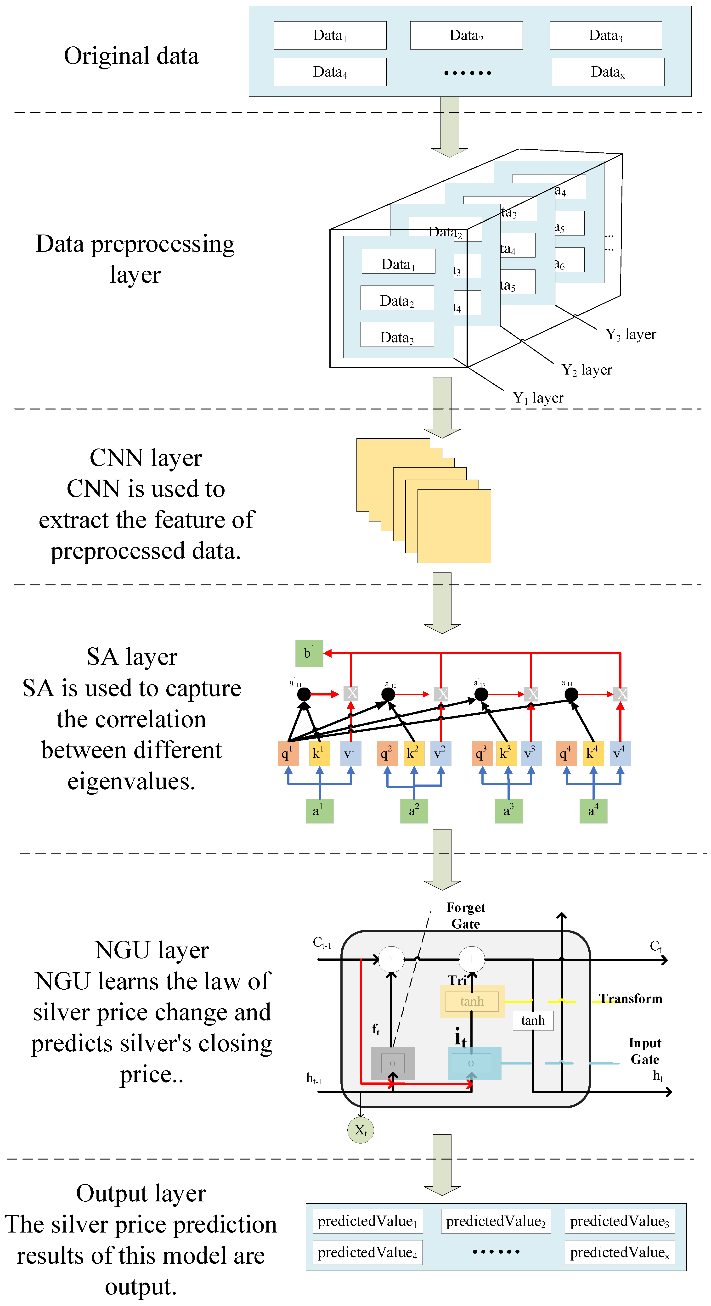
The integral structure of the CNN-SA-NGU model for silver closing price prediction is shown in Figure 3.
Data preprocessing layer: Delete the data not needed for training (including trade_date, duplicate data, invalid data, and so on) in the original data set. Standardize the data in the data set, and convert the data of different specifications to the same value interval so as to reduce the influence of distribution difference on model training.
CNN layer: By convolution operation on the input data, the data’s characteristics are extracted. The output of the CNN layer is passed to the SA layer as new input data.
SA layer: By calculating the feature data transmitted from the CNN layer, the weight coefficients are allocated, and new feature vectors are obtained.
NGU layer: This layer learns the law of silver price change and predicts silver’s closing price.
Output layer: Through the inverse normalization operation of the data output from the NGU layer, the silver price prediction results of this model are output.

4. Experiment

4.1. Experimental Environment

The hardware environment and software environment of this experiment are shown in Table 1.

4.2. Data Acquisition

In this experiment, the silver futures trading data of the Shanghai futures exchange from 5 January 2015 to 30 November 2022 are selected as experimental data. A total of 1925 pieces of data were collected. All the data collected in this experiment are obtained from the third-party data interface of the Tushare website, which is a data service platform. Silver futures price data are shown in Table 2.
The trade_date in the table indicates the opening time; the open represents the silver opening price; the high represents the highest silver price; the low represents the lowest silver price; the close represents the silver closing price; the change represents a rise or fall in value; the settle represents the settlement price; the vol represents volume; the oi represents operating income.
We select the S&P 500 index (SPX), the Dow Jones industrial average (US30), the Nasdaq 100 index (NAS100), the U.S. dollar index (USDI), the gold futures (AU), Shanghai stock index (SSI) as factors affecting silver price. The original data of silver price impact factors are shown in Table 3.

4.3. Data Preprocessing

The silver price data selected in this paper come from the trading data of Shanghai futures trading. The Shanghai futures exchange suspends trading on Saturdays and Sundays and on corresponding Chinese legal holidays. Therefore, there is no silver trading data on the corresponding date. SPX, US30, NAS100, USDI, and AU, which affect silver prices, are international market trading data. The legal working days of international exchanges are different from those in China. Therefore, there will be silver trading data on a certain day, but there are no corresponding impact factor data. For the missing impact factor data of a certain day, take the average value of the data of the previous day and the previous two days to fill in the missing data value. If the impact factor’s trading data of a particular day exist, but the silver trading data do not, the impact factor’s trading data will be deleted. The first duplicate data will be deleted when two experimental data are duplicated. If invalid trading data exist, they will be deleted.
The trade_date has no training significance in the original data, so the column data are deleted. In the original data of silver, the sample values of different characteristics are quite different. When the features have different value ranges, it will take a long time to reach the optimal local value or the optimal global value when the model is updated by the gradient. Data standardization refers to scaling the original data to eliminate the dimensional difference of the original data. That is, each index value is in the same quantity level to reduce the impact of excessive differences of orders of magnitude on model training. Z-score normalization is used for preprocessing the original data. After the standardization of the data, all the feature data sizes are in the same specific interval. Therefore, it is convenient to compare and weigh the characteristic data of different units or orders of magnitude and accelerate the convergence of the training model.
In this experiment, the first 1155 data are selected as training data, 385 data from 1155 to 1540 are used as verification data, and the remaining 385 data are used as test data.

4.4. Model Parameters

In this paper, the parameters of different models are determined by using the grid search method. By comparing the performance results obtained from different parameters, the optimal parameter combination is finally determined. In this experiment, fourteen models are compared. The important parameters of the fourteen models are shown in Table 4.

4.5. Model Comparison

To certify the validity of the CNN-SA-NGU, the prediction results of this model are compared with those of other models. The evaluation indexes of the experiment are MAE, EVS, R 2 , and training time. The results show that the CNN-SA-NGU is better than other models. The experimental results are shown in Table 5.
(1)
Comparison of Prophet, SVR, ARIMA, MLP, LSTM, Bi-LSTM, GRU, and NGU
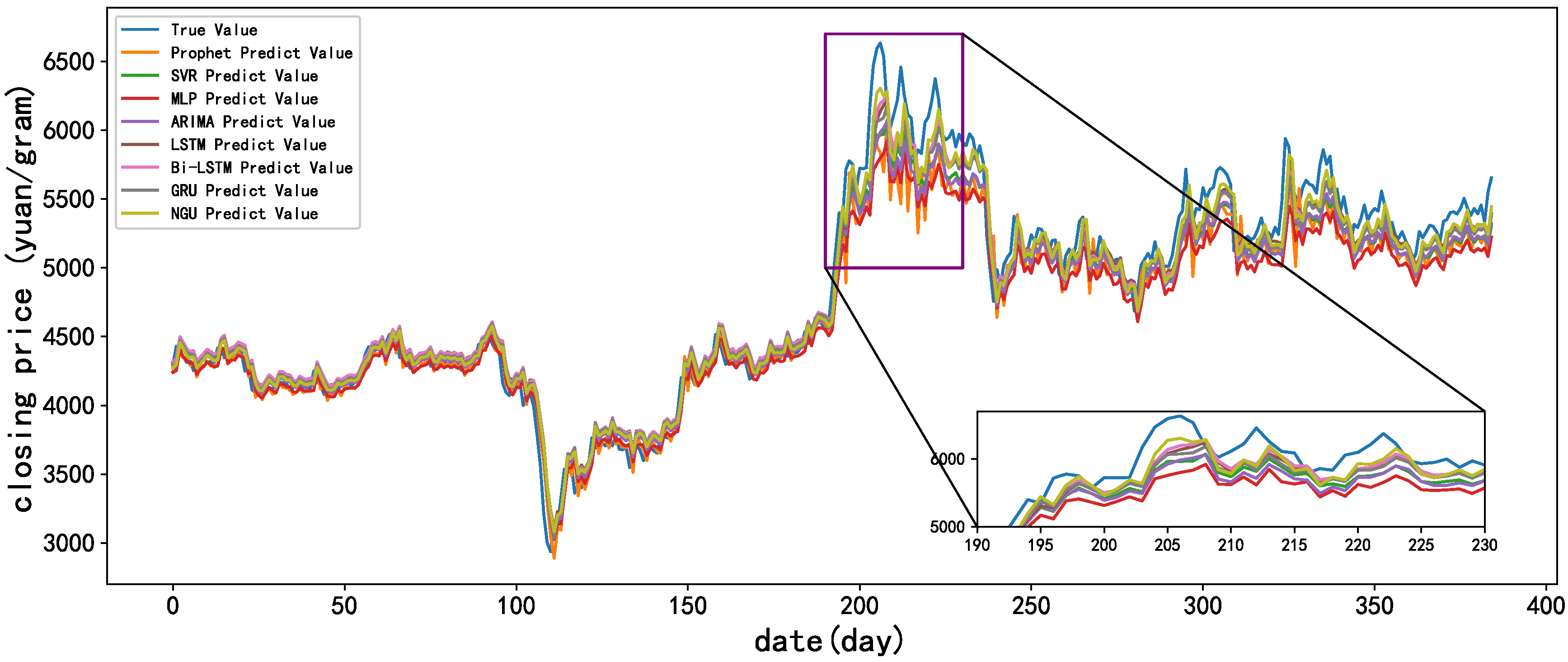
The fitting degrees of traditional machine learning algorithms SVR, ARIMA, and MLP in silver price prediction are only 0.903835, 0.907148, and 0.837680, respectively, which are poorer compared with other deep learning models. Traditional machine learning methods have poor nonlinear fitting ability. The processing of special values in data sets is not good enough, which leads to poor prediction results of the silver closing price. LSTM, Bi-LSTM, and GRU are variants of the RNN. The structure of the NGU is simple, and the training parameters are few, so the training time is greatly shortened. NGU learns the experience of the previous time to process the input data of the current time, which improves the prediction accuracy of the model. The Tri conversion module behind the NGU input gate changes the output value to alleviate the gradient disappearance and gradient explosion problems. The fitting degree of the NGU is 0.013743 higher than LSTM and 0.016974 higher than GRU. In terms of training time, NGU is 171.837 s faster than LSTM. NGU is 55.265 s faster than GRU. The comparison between the true values and the predicted results of Prophet, SVR, MLP, ARIMA, LSTM, Bi-LSTM, GRU, and NGU is shown in Figure 4.
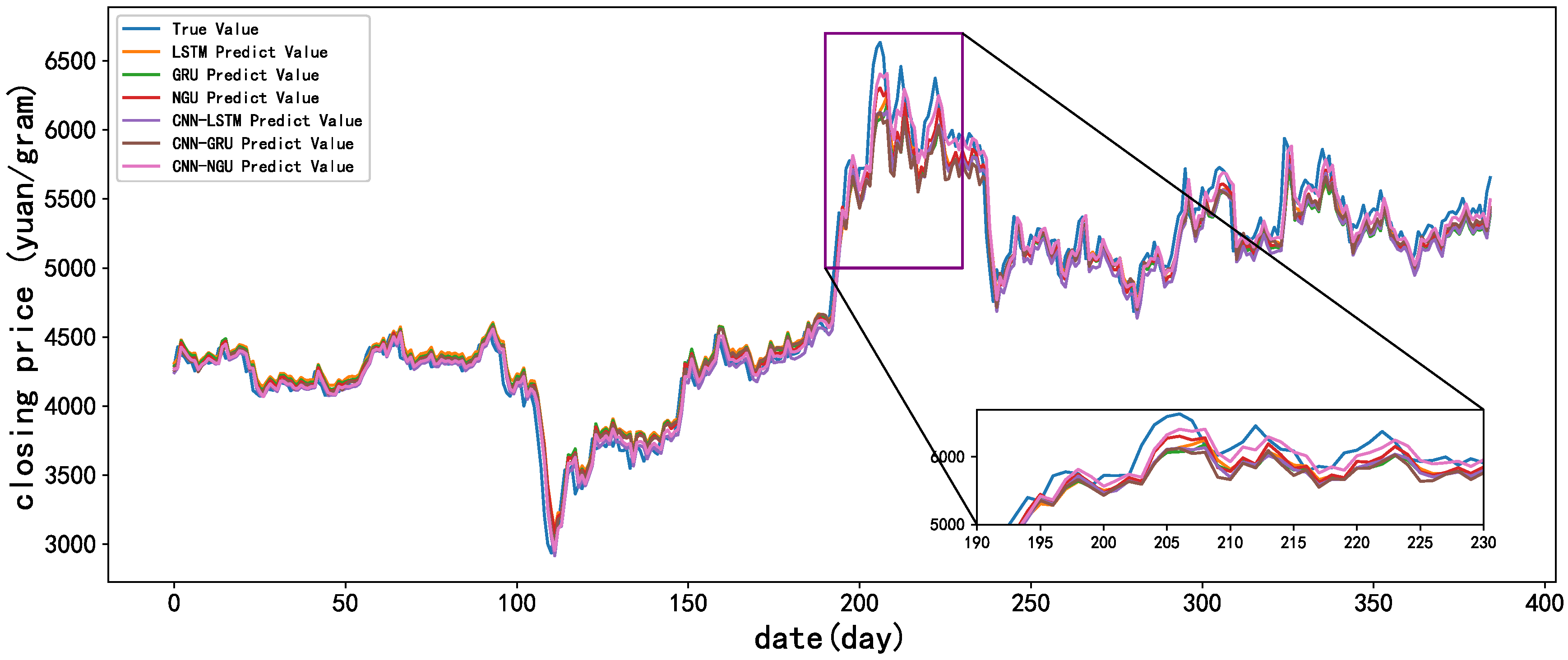
The CNN extracts the features of silver data and outputs the convolution results to the NGU for learning. Through the convolution of the CNN layer, we can better extract the features from the original data. It is beneficial to the learning of the NGU and improves the model’s prediction accuracy. After the convolution operation, the NGU directly learns the feature data without learning the rules from the original data. It shortens the training time to a certain extent. The CNN is combined with LSTM, GRU, and NGU to form a new silver forecasting hybrid model. The prediction results of CNN-LSTM, CNN-GRU, and CNN-NGU are much better than those without the CNN. The fitting degree of CNN-NGU is 0.009816 higher than the NGU. The comparison between the true values and the predicted results of LSTM, GRU, NGU, CNN-LSTM, CNN-GRU, and CNN-NGU is shown in Figure 5.
(2)
Comparison of CNN-LSTM, CNN-GRU, and CNN-NGU
The prediction fitting degree of CNN-NGU is 0.018993 higher than CNN-LSTM and 0.019479 higher than CNN-GRU. CNN-NGU’s training time is 145.121 s faster than CNN-LSTM. The comparison of prediction results of CNN-LSTM, CNN-GRU, and CNN-NGU models is shown in Figure 6.
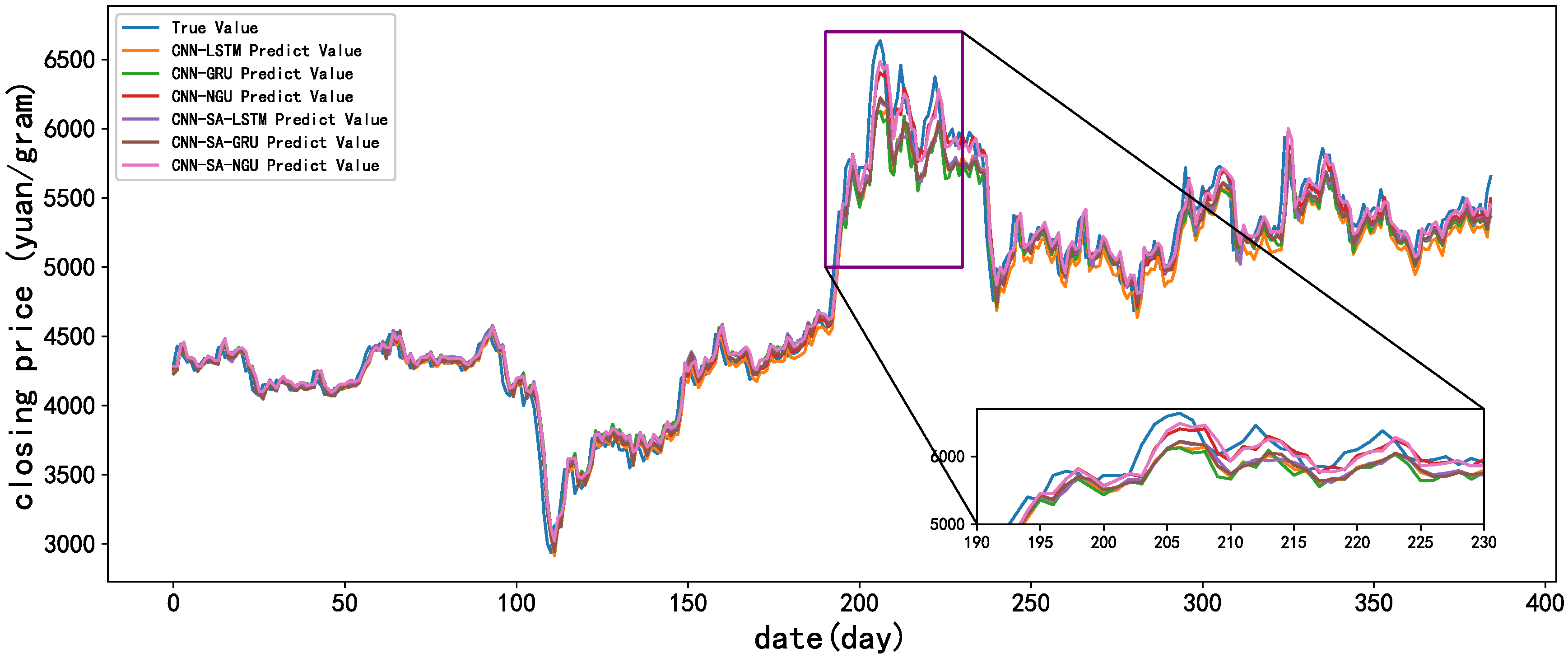
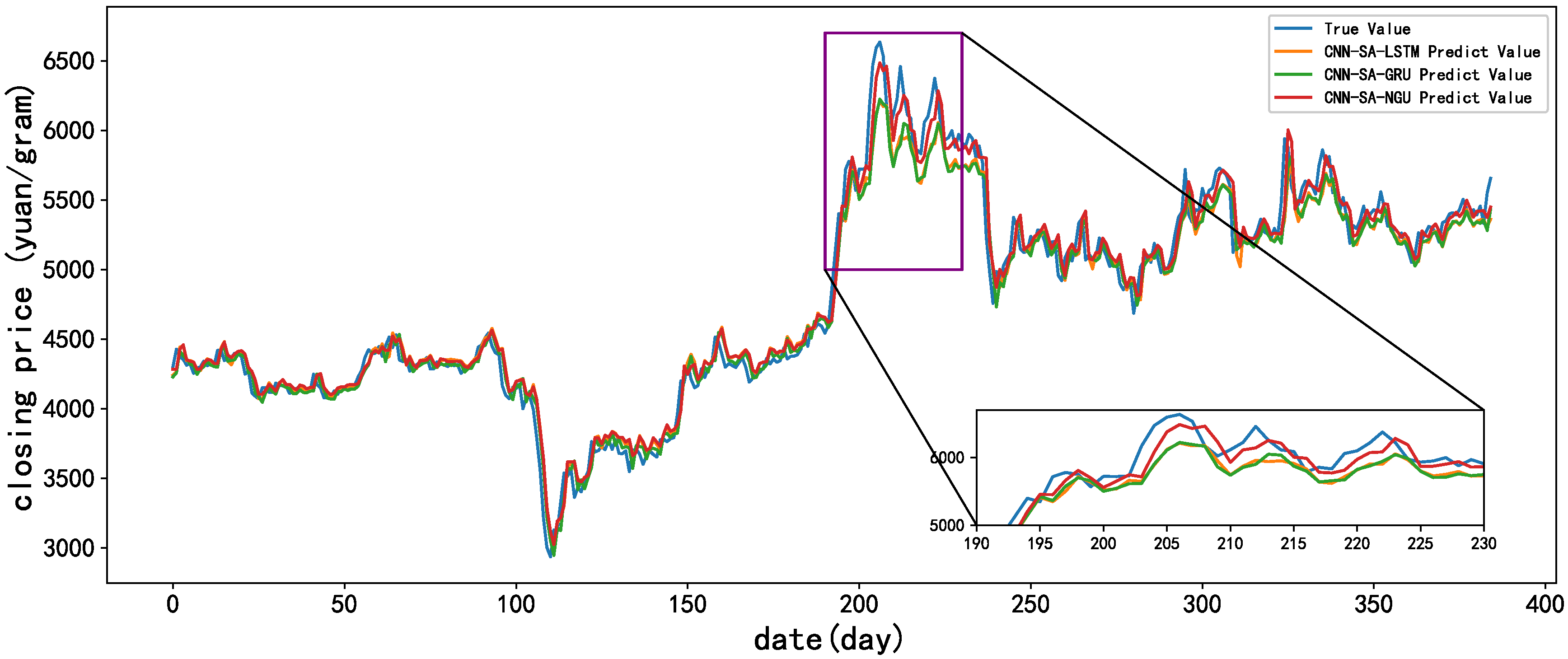
The SA mechanism processes the feature data after the convolution of the CNN convolution layer. The SA layer determines the importance of different feature data by calculation. The characteristic data that have a great influence on the prediction results are given a larger weight factor. Feature data with less influence on prediction results are given smaller weight factors. Through the treatment of SA, different eigenvalues are given different weight factors. By reassigning different weight coefficients to different data, the subsequent gated unit can learn which data have a greater impact on the prediction result. It is beneficial to NGU to learn so as to better predict the closing price of silver. The fitting degree of CNN-SA-LSTM is 0.008147 higher than CNN-LSTM, and the MAE value is 11.108407 lower. The fitting degree of CNN-SA-GRU is 0.013341 higher than CNN-GRU, and the MAE value is 10.607317 lower. The fitting degree of CNN-SA-NGU is 0.006484 higher than CNN-NGU, and the MAE value is 9.378917 lower. The comparison between the true values and the predicted results of CNN-LSTM, CNN-GRU, CNN-NGU, CNN-SA-LSTM, CNN-SA-GRU, and CNN-SA-NGU is shown in Figure 7.
(3)
Comparison of CNN-SA-LSTM, CNN-SA-GRU, and CNN-SA-NGU
Among the three models of CNN-SA-LSTM, CNN-SA-GRU, and CNN-SA-NGU, the performance of CNN-SA-NGU is the best. The fitting degree of CNN-SA-NGU is 0.01733 higher than CNN-SA-LSTM and 0.012622 higher than CNN-SA-GRU. The training time of CNN-SA-NGU is 95.265 s shorter than CNN-SA-LSTM. The true values are compared with the predicted results of CNN-SA-LSTM, CNN-SA-GRU, and CNN-SA-NGU models, as shown in Figure 8.

4.6. Generalization Ability of Model

CNN-SA-NGU model has good generalization ability. It shows good performance in silver price prediction and is suitable for forecasting other time series data such as ETFs, gold futures, and stocks. The following experiments are carried out with gold futures and Shanghai stock composite index data. The experimental results of forecasting gold futures prices are shown in Table 6. The experimental results of forecasting the Shanghai stock composite index are shown in Table 7.
Through the above two tables, we can see that the CNN-SA-NGU model has good generalization ability.

5. Discussion

Compared with ten other silver price prediction models, the performance of the CNN-SA-NGU is the best. Compared with SVR, MLP, LSTM, and GRU, the NGU presented in this paper has a better performance in MAE, EVS, R 2 , and training time. Adding a CNN to the model improves the ability to extract feature data. The SA layer is added to the model to redistribute the weights of different feature data. It is beneficial for NGU learning. The NGU learns from the previous training experience to deal with the input data at the current time, which improves the nonlinear fitting ability of the model. The CNN-SA-NGU model can achieve higher prediction accuracy for the following reasons:
(1)
The NGU uses the original learning experience fully to enhance the processing ability of the input data at the current time, thus improving the nonlinear fitting ability of the model. The Tri conversion module changes the range of output value by processing the output data of the input gate, thus alleviating the problems of gradient disappearance and gradient explosion.
(2)
With the addition of the SA mechanism, the feature data that significantly influence the prediction results can be well identified. The SA mechanism reallocates the weights of different feature data through calculation. Additionally, a higher weight factor is assigned to the feature data, which benefits the NGU’s learning.
(3)
By adding the CNN convolution layer, the model’s feature extraction ability is improved. The hidden features between data can be mined by the CNN.

6. Conclusions

This paper presents a novel hybrid model of CNN-SA-NGU for silver closing price prediction. The CNN convolution layer solves the problem of incomplete feature data extraction in traditional models to some extent. After introducing the SA mechanism, the relationship between different feature data can be learned, thus increasing the sensitivity of the model to feature data. The structure of the NGU is simple, and the training parameters are few, greatly reducing the training time. The Tri conversion module of the NGU deals with the output data of the input gate, which ameliorates the problems of gradient disappearance and gradient explosion. NGU fully learns the experience of the previous time and deals with the input data at the current time, which improves the model’s nonlinear fitting ability and improves its prediction accuracy. The comparative experiments show that the performance of CNN-SA-NGU is better than other models, but the model has the shortcoming of not fitting some extreme values in the data set well.
Our future research directions are as follows:
(1)
Currently, the model only takes scalar data such as SPX, US30, NAS100, USDI, AU, and SSI as the influencing factors of the silver price. However, some factors still affect the silver price, such as investors’ psychology, the formulation of laws, and political events. In future research, we should use natural language processing technology to quantify political events such as policy changes and wars as influencing factors and input them into the prediction model to improve prediction accuracy.
(2)
We will further attempt to improve the SA model to make the weight coefficient allocation of the importance of feature data more reasonable.

Author Contributions

Conceptualization, H.W.; methodology, H.W. and J.W.; software, B.D. and X.L.; validation, N.Y.; investigation, N.Y. and B.D.; writing—original draft preparation, B.D. and N.Y. writing—review and editing, J.W. and H.W.; visualization, B.D. and X.L.; supervision, H.W. and J.W.; project administration, B.D. and N.Y.; funding acquisition, H.W. and J.W. All authors have read and agreed to the published version of the manuscript.

Funding

This research was funded by the Scientific Research Project Foundation for High-level Talents of the Xiamen Ocean Vocational College under Grant KYG202102, and Innovation Foundation of Hebei Intelligent Internet of Things Technology Innovation Center under Grant AIOT2203.

Institutional Review Board Statement

Not applicable.

Informed Consent Statement

Not applicable.

Data Availability Statement

Data are available on request due to restrictions privacy. The data presented in this study are available on request from the corresponding author.

Conflicts of Interest

The authors declare no conflict of interest.

Abbreviations

NO.AbbreviationFull Name
1ARIMAautoregressive integrated moving average
2AUgold futures
3Bi-LSTMbi-directional long short-term memory
4CNNconventional neural network
5EVSexplained variance score
6GRUgated recurrent unit
7GRUNNgate recurrent unit neural network
8ICAindependent component analysis
9LSTMlong short-term memory
10MAEmean absolute error
11MLPmulti-layer perceptron
12NAS100Nasdaq 100 index
13NGUnew gated unit
14R2r squared
15RNNrecurrent neural network
16S2SANsentence-to-sentence attention network
17SAself-attention
18SPXS&P 500 index
19SSIShanghai stock index
20SVMsupport vector machine
21SVRsupport vector regression
22US30Dow Jones industrial average
23USDIU.S. dollar index
24VMDvariational mode decomposition

References

  1. Kim, T.; Kim, H.Y. Forecasting stock prices with a feature fusion LSTM-CNN model using different representations of the same data. PLoS ONE 2019, 14, e0212320. [Google Scholar] [CrossRef] [PubMed] [Green Version]
  2. Cunado, J.; Gil-Alana, L.A.; Gupta, R. Persistence in trends and cycles of gold and silver prices: Evidence from historical data. Phys. A Stat. Mech. Its Appl. 2019, 514, 345–354. [Google Scholar] [CrossRef] [Green Version]
  3. Apergis, I.; Apergis, N. Silver prices and solar energy production. Environ. Sci. Pollut. Res. 2019, 26, 8525–8532. [Google Scholar] [CrossRef]
  4. Kotsiantis, S.B. Decision trees: A recent overview. J. Artif. Intell. Rev. 2013, 39, 261–283. [Google Scholar] [CrossRef]
  5. Heo, J.; Jin, Y.Y. SVM based Stock Price Forecasting Using Financial Statements. J. Korea Ind. Inf. Syst. Soc. 2015, 21, 167–172. [Google Scholar] [CrossRef]
  6. Liu, R.; Liu, L. Predicting housing price in China based on long short-term memory incorporating modified genetic algorithm. Soft Comput. 2019, 23, 11829–11838. [Google Scholar] [CrossRef]
  7. Yu, Y.; Si, X.S.; Hu, C.H.; Zhang, J.X. A Review of Recurrent Neural Networks: LSTM Cells and Network Architectures. Neural Comput. 2019, 31, 1235–1270. [Google Scholar] [CrossRef] [PubMed]
  8. Li, G.N.; Zhao, X.W.; Fan, C.; Fang, X.; Li, F.; Wu, Y.B. Assessment of long short-term memory and its modifications for enhanced short-term building energy predictions. J. Build. Eng. 2021, 43, 103182. [Google Scholar] [CrossRef]
  9. Liu, Y.; Zhang, X.M.; Zhang, Q.Y.; Li, C.Z.; Huang, F.R.; Tang, X.H.; Li, X.J. Dual Self-Attention with Co-Attention Networks for Visual Question Answering. Pattern Recognit. 2021, 117, 107956. [Google Scholar] [CrossRef]
  10. Humphreys, G.W.; Sui, J. Attentional control and the self: The Self-Attention Network (SAN). Cogn. Neurosci. 2015, 7, 5–17. [Google Scholar] [CrossRef]
  11. Lin, Z.H.; Li, M.M.; Zheng, Z.B.; Cheng, Y.Y.; Yuan, C. Self-Attention ConvLSTM for Spatiotemporal Prediction. In Proceedings of the AAAI Conference on Artificial Intelligence, New York, NY, USA, 7–12 February 2020; pp. 11531–11538. [Google Scholar] [CrossRef]
  12. Yuan, F.C.; Lee, C.H.; Chiu, C.C. Using Market Sentiment Analysis and Genetic Algorithm-Based Least Squares Support Vector Regression to Predict Gold Prices. Int. J. Comput. Intell. Syst. 2020, 13, 234–246. [Google Scholar] [CrossRef] [Green Version]
  13. Aksehir, Z.D.; Kilic, E. How to handle data imbalance and feature selection problems in CNN-based stock price forecasting. IEEE Access 2020, 10, 31297–31305. [Google Scholar] [CrossRef]
  14. He, C.M.; Kang, H.Y.; Yao, T.; Li, X.R. An effective classifier based on convolutional neural network and regularized extreme learning machine. Math. Biosci. Eng. 2019, 16, 8309–8321. [Google Scholar] [CrossRef] [PubMed]
  15. Chen, W.B.; Lu, Y.; Ma, H.; Chen, Q.L.; Wu, X.B.; Wu, P.L. Self-attention mechanism in person re-identification models. Multimed. Tools Appl. 2022, 81, 4649–4667. [Google Scholar] [CrossRef]
  16. Yan, R.; Liao, J.Q.; Yang, J.; Sun, W.; Nong, M.Y.; Li, F.P. Multi-hour and multi-site air quality index forecasting in Beijing using CNN, LSTM, CNN-LSTM, and spatiotemporal clustering. Expert Syst. Appl. 2021, 169, 114513. [Google Scholar] [CrossRef]
  17. Vidal, A.; Kristjanpoller, W. Gold volatility prediction using a CNN-LSTM approach. Expert Syst. Appl. 2020, 157, 113481. [Google Scholar] [CrossRef]
  18. Jianwei, E.; Ye, J.M.; Jin, H.H. A novel hybrid model on the prediction of time series and its application for the gold price analysis and forecasting. Phys. A Stat. Mech. Its Appl. 2019, 527, 121454. [Google Scholar] [CrossRef]
  19. Liu, Y.; Zhang, Z.L.; Liu, X.; Wang, L.; Xia, X.H. Deep Learning Based Mineral Image Classification Combined with Visual Attention Mechanism. IEEE Access 2021, 9, 98091–98109. [Google Scholar] [CrossRef]
  20. Liu, J.J.; Yang, J.K.; Liu, K.X.; Xu, L.Y. Ocean Current Prediction Using the Weighted Pure Attention Mechanism. J. Mar. Sci. Eng. 2022, 10, 592. [Google Scholar] [CrossRef]
  21. Kim, G.; Shin, D.H.; Choi, J.G.; Lim, S. A Deep Learning-Based Cryptocurrency Price Prediction Model That Uses On-Chain Data. IEEE Access 2022, 10, 56232–56248. [Google Scholar] [CrossRef]
  22. Wang, P.; Li, J.N.; Hou, J.R. S2SAN: A sentence-to-sentence attention network for sentiment analysis of online reviews. Decis. Support Syst. 2021, 149, 113603. [Google Scholar] [CrossRef]
  23. Li, Q.B.; Yao, N.M.; Zhao, J.; Zhang, Y.A. Self attention mechanism of bidirectional information enhancement. Appl. Intell. 2022, 52, 2530–2538. [Google Scholar] [CrossRef]
  24. Liang, Y.H.; Lin, Y.; Lu, Q. Forecasting gold price using a novel hybrid model with ICEEMDAN and LSTM-CNN-CBAM. Expert Syst. Appl. 2022, 206, 117847. [Google Scholar] [CrossRef]
  25. Chen, W.J. Estimation of International Gold Price by Fusing Deep/Shallow Machine Learning. J. Adv. Transp. 2022, 2022, 6211861. [Google Scholar] [CrossRef]
  26. Chen, S.; Ge, L. Exploring the attention mechanism in LSTM-based Hong Kong stock price movement prediction. Quant. Financ. 2019, 19, 1507–1515. [Google Scholar] [CrossRef]
  27. Zeng, C.; Ma, C.X.; Wang, K.; Cui, Z.H. Parking Occupancy Prediction Method Based on Multi Factors and Stacked GRU-LSTM. IEEE Access 2022, 10, 47361–47370. [Google Scholar] [CrossRef]
  28. Deng, L.J.; Ge, Q.X.; Zhang, J.X.; Li, Z.H.; Yu, Z.Q.; Yin, T.T.; Zhu, H.X. News Text Classification Method Based on the GRU_CNN Model. Int. Trans. Electr. Energy Syst. 2022, 2022, 1197534. [Google Scholar] [CrossRef]
  29. Sun, W.W.; Guan, S.P. A GRU-based traffic situation prediction method in multi-domain software defined network. PeerJ Comput. Sci. 2022, 8, e1011. [Google Scholar] [CrossRef]
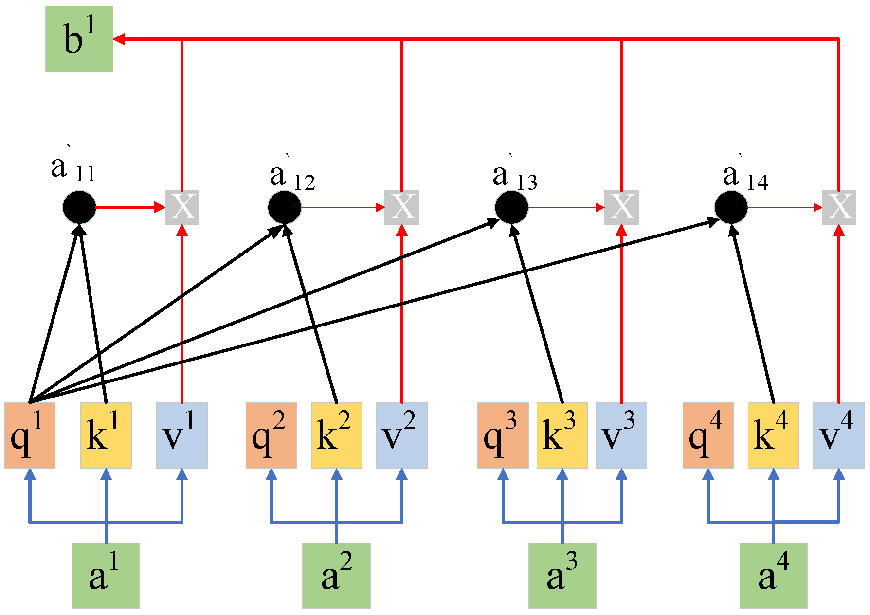
Figure 1. The principle of the SA mechanism.
Processes 11 00862 g001
Figure 2. NGU structure diagram.
Processes 11 00862 g002
Figure 3. CNN-SA-NGU structure diagram.
Processes 11 00862 g003
Figure 4. Comparison of true values with Prophet, SVR, ARIMA, MLP, LSTM, Bi-LSTM, GRU, and NGU prediction results.
Processes 11 00862 g004
Figure 5. Comparison between true values and predicted results of LSTM, GRU, NGU, CNN-LSTM, CNN-GRU, and CNN-NGU.
Processes 11 00862 g005
Figure 6. Comparison of true values with CNN-LSTM, CNN-GRU, and CNN-NGU prediction results.
Processes 11 00862 g006
Figure 7. Comparison of true values with CNN-LSTM, CNN-GRU, CNN-NGU, CNN-SA-LSTM, CNN-SA-GRU, and CNN-SA-NGU predictions.
Processes 11 00862 g007
Figure 8. Comparison of true values with CNN-SA-LSTM, CNN-SA-GRU, and CNN-SA-NGU predictions.
Processes 11 00862 g008
Table 1. Experimental environment.
Environment TypeProject NameValue
Hardware environmentOperating systemWindows 11
CPUIntel i7-12700H 2.30 GHz
Memory16GB
Graphics cardRTX 3070Ti
Software environmentDevelopment toolsPyCharm 2020 1.3
Programming languagePython3.7.0
Basic platformAnaconda4.5.11
Learning frameworkkeras2.1.0 and TensorFlow 1.14.0
Table 2. Silver futures price data items.
Trade_DateOpenHighLowCloseChangeSettleVolOi
5 January 20153498351634783507−1735005137980041042000
6 January 2015349035663462355454351721999720045015800
7 January 2015354435963530355437355618658760040197400
8 January 20153540357835373548−8355814341220041246400
9 January 20153568358635443555−3356214158900040017000
Table 3. Original data of silver price impact factors.
Trade_DateSPXUS30NAS100USDIAUSSI
5 January 20152000.63173624102.899911648242.153350.519
6 January 20152026.38175904155.899911655244.453351.446
7 January 20152060.1299178814236.899911684245.253373.9541
8 January 20152041.88177204207.600111690244.53293.4561
9 January 20152041.88177204207.600111633245.153285.4121
Table 4. Model parameters.
ModelLayerParameters
ProphetProphetinterval_width = 0.8
SVRSVRkernel = ‘linear’, epsilon = 0.07, C = 4
MLPMLPactivation = “tanh”
ARIMAARIMAdynamic = false
LSTMLSTMactivation = ‘tanh’, units = 128
Bi-LSTMBi-LSTMactivation = ‘tanh’, units = 128
GRUGRUactivation = ‘tanh’, units = 128
NGUNGUactivation = ‘tanh’, units = 128
CNN-LSTMConv1D
LSTM
filters = 16, kernel_size = 3,
activation = ‘tanh’, units = 128
CNN-GRUConv1D
GRU
filters = 16, kernel_size = 3,
activation = ‘tanh’, units = 128
CNN-NGUConv1D
NGU
filters = 16, kernel_size = 3,
activation = ‘tanh’, units = 128
CNN-SA-LSTMConv1D
SA
LSTM
filters = 16, kernel_size = 3,
initializer = ‘uniform’,
activation = ‘tanh’, units = 128
CNN-SA-GRUConv1D
SA
GRU
filters = 16, kernel_size = 3,
initializer = ‘uniform’,
activation = ‘tanh’, units = 128
CNN-SA-NGUConv1D
SA
NGU
filters = 16, kernel_size = 3,
initializer = ‘uniform’,
activation = ‘tanh’, units = 128
Table 5. Experimental results.
ModelMAEEVS R 2 Training Time (t/s)
Prophet176.8297650.8995820.86499973.432
SVR182.0386980.9282410.90383550.824
MLP190.1681720.8488850.8376805.598
ARIMA168.6550630.9071590.90714824.946
LSTM116.5393920.9405640.940126450.684
Bi-LSTM119.6703330.9417580.9412391306.247
GRU118.7483770.9396360.936895334.112
NGU103.9601580.9552760.953869278.847
CNN-LSTM113.7729530.9568820.944692398.622
CNN-GRU108.0318830.9470180.944206272.832
CNN-NGU97.2776880.9656630.963685253.501
CNN-SA-LSTM102.6645460.9541180.952839428.042
CNN-SA-GRU97.4245660.9605150.957547328.642
CNN-SA-NGU87.8987710.9707450.970169332.777
Table 6. The experimental results of the forecasting table of gold futures prices.
ModelMAEEVS R 2 Training Time (t/s)
Prophet7.3283860.8896230.84962361.752
SVR5.7671650.9356150.91576445.185
MLP7.0122490.9019120.8611669.969
ARIMA6.7576690.9416290.89824228.905
LSTM4.8719390.9429180.939975479.996
Bi-LSTM4.8557960.9449590.9439411098.907
GRU4.7362810.9465340.944854323.123
NGU4.8145740.9725030.955799279.747
CNN-LSTM4.6255110.9622450.951108465.302
CNN-GRU4.5283360.9597780.953008306.796
CNN-NGU4.0328190.9716740.966912257.907
CNN-SA-LSTM4.2640180.9608520.956380483.592
CNN-SA-GRU4.1855530.9590460.959038374.097
CNN-SA-NGU3.6285490.9725740.971670367.560
Table 7. The experimental results of forecasting the Shanghai stock composite index.
ModelMAEEVS R 2 Training Time (t/s)
Prophet47.5455720.9023150.90135663.558
SVR31.2346450.9599480.95888736.740
MLP40.5418820.9425510.9339078.011
ARIMA39.2516000.9556440.95507625.791
LSTM28.9448380.9683790.967678466.249
Bi-LSTM28.4091770.9698490.9689161327.013
GRU27.0716430.9713950.970907304.327
NGU26.5737120.9791910.975161290.925
CNN-LSTM28.2790520.9775640.972431489.508
CNN-GRU25.7673930.9782230.975720273.203
CNN-NGU23.4523980.9797900.979602256.740
CNN-SA-LSTM27.7679570.9792280.978946495.647
CNN-SA-GRU25.9579190.9831230.980307386.600
CNN-SA-NGU22.6398940.9848260.984815377.040
Disclaimer/Publisher’s Note: The statements, opinions and data contained in all publications are solely those of the individual author(s) and contributor(s) and not of MDPI and/or the editor(s). MDPI and/or the editor(s) disclaim responsibility for any injury to people or property resulting from any ideas, methods, instructions or products referred to in the content.