Economic Model Predictive Control of Nonlinear Systems Using Online Learning of Neural Networks

Abstract

This work focuses on the development of a Lyapunov-based economic model predictive control (LEMPC) scheme that utilizes recurrent neural networks (RNNs) with an online update to optimize the economic benefits of switched non-linear systems subject to a prescribed switching schedule. We first develop an initial offline-learning RNN using historical operational data, and then update RNNs with real-time data to improve model prediction accuracy. The generalized error bounds for RNNs updated online with independent and identically distributed (i.i.d.) and non-i.i.d. data samples are derived, respectively. Subsequently, by incorporating online updating RNNs within LEMPC, probabilistic closed-loop stability, and economic optimality are achieved simultaneously for switched non-linear systems accounting for the RNN generalized error bound. A chemical process example with scheduled mode transitions is used to demonstrate that the closed-loop economic performance under LEMPC can be improved using an online update of RNNs.

1. Introduction

An economic model predictive control (EMPC) that addresses economic considerations within process control has attracted considerable attention in the control community over recent decades. Model predictive control (MPC) is applied in a wide variety of applications due to its ability to handle hard constraints on system states and manipulated inputs. The key idea of MPC is to compute an optimal input sequence using state feedback at the current sampling instant, and only the first input is fed to the system. Typically, a quadratic cost function is used in tracking MPC schemes to penalize the deviation of predicted system states and manipulated inputs from their steady-state values over a finite prediction horizon, such that the system is driven to its desired steady-state by minimizing the quadratic cost function. Unlike the steady-state operation of conventional tracking MPC schemes, EMPC generally uses a non-quadratic objective function to operate in a dynamic fashion (off steady-state) by optimizing process economics. Many research works have been developed to address closed-loop stability, economic optimization considerations, and model uncertainty for non-linear systems under EMPC (e.g., [1,2,3,4,5,6]).

Since, in real life, dynamical processes often involve mode transitions that may arise due to various reasons (e.g., actuator/sensor faults, feedback changes, and changes in environmental factors), it gives rise to an important research subject of switched systems. A class of systems with multiple switching modes is termed switched systems, whose active mode is determined by a switching signal. Switch systems have wide applications in engineering practice (e.g., mobile robots [7], electrical circuits [8], and flight control [9]). Control and optimization of switched systems have been extensively explored using methods in terms of Lyapunov stability theory [10,11], dwell-time [12,13], and linear matrix inequality [14]. In [15], a Lyapunov-based MPC framework was presented to stabilize switched non-linear systems that execute mode transitions at the prescribed switching times. Following this direction, in [16], a Lyapunov-based EMPC method was proposed to address the stabilization and economic optimality of switched non-linear systems subject to a prescribed switching schedule.

An accurate process model is a key requirement for achieving the desired control performance under EMPC. To this end, the above EMPC schemes often assume that the process model with the desired prediction accuracy can be obtained using first-principles modeling approaches. However, capturing the non-linear dynamics of complex and large-scale systems based on first-principles modeling approaches can be cumbersome and inaccurate when the physio-chemical phenomena of the system are not well-understood. Machine learning (ML) algorithms have shown great success in a variety of application domains in recent years, e.g., the resolving-power domination number of probabilistic neural networks was investigated in [17], and Gaussian process models were used to capture the dynamics of non-linear processes with unknown dynamics in [18] and with time-varying dynamics in [19]. As a powerful black box modeling tool among various ML algorithms, RNNs have achieved astonishing results in ML-based control for non-linear systems since they can approximate non-linear dynamics based on time-series data [20,21,22]. In [23], an RNN model was constructed offline to predict future states for EMPC that optimize economic benefits for non-linear systems while maintaining closed-loop stability. However, since ML models are generally trained offline to model non-linear systems under normal operation (i.e., without model uncertainty) using historical operational data, the resulting offline-trained ML models may not well approximate real-time non-linear dynamics subject to model uncertainty. Therefore, the presence of model uncertainty could result in degradation of the control performance of real-world non-linear processes under ML-based EMPC with offline-trained ML models. In [24], online learning with event-triggered and error-triggered mechanisms was applied to update ML models based on real-time data to learn model uncertainty, thus improving the control performance of non-linear systems subject to model uncertainty under ML-based EMPC.

Many works have been developed to integrate online learning models with a control design for non-linear processes (e.g., [25,26,27,28]). Although online learning models have shown their effectiveness in improving the prediction accuracy and control performance of non-linear processes, characterizing their generalization performance on the unseen testing set remains a critical challenge for real-time implementation of online ML-based controllers in practice. The generalized error bound is widely used to evaluate how an ML model developed using the training set can generalize well to the unseen testing set. The generalized error bound for online ML models has been developed in [29,30,31] by assuming that the online learner receives a data sequence generated in an i.i.d. manner. Certain efforts have been made in [32,33] to remove the i.i.d. assumption on training data points, for which the generalized error bound for online ML models updated with a set of non-i.i.d. data points has been derived. In our previous work, the generalized error bounds for RNNs updated online using i.i.d. and non-i.i.d. data points were established in [34,35], respectively, and the error bounds were utilized to derive closed-loop stability properties for switched non-linear systems without and with process disturbances under online updating RNN-based MPC. However, at this stage, it remains unclear how online learning RNNs can be integrated with EMPC to optimize economic benefits for switched non-linear systems while maintaining closed-loop stability.

To fill this research gap, this work aims to incorporate online learning RNNs into LEMPC to address closed-loop stability and economic optimality for switched non-linear systems operating under scheduled mode transitions. Specifically, the notation, class of switched non-linear systems, and the developments of RNNs are presented in Section 2. The generalized error bounds for RNNs updated online using i.i.d. and non-i.i.d. training data points are derived in Section 3. In Section 4, an LEMPC scheme that integrates online updating RNNs is proposed for switched non-linear systems involving process disturbances, under which probabilistic closed-loop stability is proved based on the RNN generalized error bound. In Section 5, a non-linear chemical process example with scheduled mode transitions is presented to demonstrate the efficacy of the proposed LEMPC scheme.

2. Preliminaries

2.1. Notation

The operators ${∥·∥}_F$ and $|·|$ are used to represent the Frobenius norm of a matrix and the Euclidean norm of a vector, respectively. The function $f(·)$ belongs to class ${\mathcal{C}}^1$ if $f(·)$ is continuously differentiable. We use the operator $“\backslash ”$ to represent set subtraction, i.e., $\mathcal{M}\backslash \mathcal{V}:=\{x\in {\mathbb{R}}^n|x\in \mathcal{M},x\notin \mathcal{V}\}$. The continuous function $f:[0,a)\to [0,\infty )$ belongs to class $\mathcal{K}$ if it satisfies $f\left(0\right)=0$ and increases strictly in its domain. $\mathbb{E}\left[X\right]$ and $\mathbb{P}\left(A\right)$ and are used to denote the expected value of a random variable X and the probability of a event A occurring, respectively. Let $a_m$ and $b_m$ be two sequences, we will write $a_m=\mathcal{O}\left(b_m\right)$ provided that $lim{sup}_{m\to \infty }\left|a_m/b_m\right|<\infty$.

2.2. Class of Switched Non-Linear Systems

In this work, a class of switched non-linear systems described by the following first-order ordinary differential equations (ODEs) is considered.

$$\begin{array}{cc}\hfill \dot{x}& =F_{\sigma \left(t\right)}(x,u_{\sigma \left(t\right)},w_{\sigma \left(t\right)})\hfill \\ \hfill & :=f_{\sigma \left(t\right)}\left(x\right)+g_{\sigma \left(t\right)}\left(x\right)u_{\sigma \left(t\right)}+h_{\sigma \left(t\right)}\left(x\right)w_{\sigma \left(t\right)}\hfill \end{array}$$

(1)

where $x\in {\mathbb{R}}^n$, $u_{\sigma \left(t\right)}\in {\mathbb{R}}^{n_u}$, and $w_{\sigma \left(t\right)}\in {\mathbb{R}}^{n_w}$ denote the vectors of system states, control inputs, and disturbances, respectively. The control input constraint is given by $u_{\sigma \left(t\right)}\in U_{\sigma \left(t\right)}$, where the set $U_{\sigma \left(t\right)}$ defines the vectors of the minimum value $u_{\sigma \left(t\right)}^{min}$ and the maximum value $u_{\sigma \left(t\right)}^{max}$ for the input constraint (i.e., $U_{\sigma \left(t\right)}:=\left\{u_{\sigma \left(t\right)}^{min}\le u_{\sigma \left(t\right)}\le u_{\sigma \left(t\right)}^{max}\right\}$). The disturbance vector is subject to the constraint $w_{\sigma \left(t\right)}\in {\mathcal{W}}_{\sigma \left(t\right)}:=\left\{|w_{\sigma \left(t\right)}|\le w_{m_{\sigma \left(t\right)}},w_{m_{\sigma \left(t\right)}}\ge 0\right\}$. The switching function $\sigma \left(t\right):[0,\infty )\to \psi$ takes a value in $\psi :=\{1,\dots ,p\}$. The number of switching modes is denoted by p. Throughout this manuscript, the notations $t_k^{out}$ and $t_k^{in}$ are used to represent the time at which the k-th mode (i.e., $k\in \psi$) of Equation (1) is switched out and in, respectively. Therefore, the state-space model of Equation (1) is denoted by $\dot{x}=F_k(x,u_k,w_k)$ with $\sigma \left(t\right)=k$ when the system operates under mode k for $t\in \left[t_k^{in},t_k^{out}\right)$. For all $k\in \psi$, $f_k(·)$, $g_k(·)$, and $h_k(·)$ are assumed to be sufficiently smooth functions of dimensions $n\times 1$, $n\times n_u$, and $n\times n_w$, respectively. Additionally, for all $k\in \psi$, we assume that $f_k\left(0\right)=0$ and the initial time $t_0$ is zero, indicating that the origin is a steady-state of Equation (1) without disturbances (i.e., the nominal system). All states are assumed to be measurable at each sampling instant $t_q=t_k^{in}+q\Delta$, where $\Delta$ is the sampling period, $q=0,1,\cdots ,N_k$, and $N_k$ is assumed to be a positive integer denoting the total number of sampling periods within $t\in [t_k^{in}$, $t_k^{out}$).

For each mode $k\in \psi$, a stabilizing controller $u_k={\Phi }_k\left(x\right)\in U_k$ (e.g., the universal Sontag control law [36]) is assumed to exist in the sense that the origin of Equation (1) without disturbances is rendered exponentially stable. Following the construction method in [37], a level set of $V_k\left(x\right)$ (denoted by ${\Omega }_{{\rho }_k}:=\left\{x\in {\mathbb{R}}^n\mid V_k\left(x\right)\le {\rho }_k\right\}$, where $0<{\rho }_k$ for $k\in \psi$) is used to represent the stability region of Equation (1) operating under mode k. Additionally, taking into account by the boundedness of $x,u_k,w_k$, the smoothness assumed for $f_k(·)$, $g_k(·)$, and $h_k(·)$, and the continuous differentiable property of $V_k\left(x\right)$, positive constants $L_{w_k}^{\prime },L_{w_k},L_{x_k}^{\prime },L_{x_k},M_k$ are assumed to exist, such that the following inequalities hold for all $x^{\prime },x\in {\Omega }_{{\rho }_k},w_k\in {\mathcal{W}}_k$, $u_k\in U_k$, $k\in \psi$:

$$\begin{array}{c}\left|F_k(x^{\prime },u_k,0)-F_k(x,u_k,w_k)\right|\le L_{w_k}\left|w_k\right|+L_{x_k}\left|x^{\prime }-x\right|\end{array}$$

(2a)

$$\begin{array}{c}\left|\frac{\partial V_k\left(x^{\prime }\right)}{\partial x}{F}_k(x^{\prime },u_k,0)-\frac{\partial V_k\left(x\right)}{\partial x}{F}_k(x,u_k,w_k)\right|\le L_{w_k}^{\prime }\left|w_k\right|+L_{x_k}^{\prime }\left|x^{\prime }-x\right|\end{array}$$

(2b)

$$\begin{array}{c}|F_k(x,u_k,w_k)|\le M_k\end{array}$$

(2c)

2.3. Recurrent Neural Networks (RNN)

As opposed to the architecture of a traditional feedforward neural network in which signals are transmitted in only one direction, information in an RNN travels in both directions (i.e., forward and backward) due to the inclusion of recurrent loops as shown in Figure 1. This enables the feedback of signals associated with previous inputs back into the network, and fosters a temporal dynamic behavior that corresponds to the numerical techniques (e.g., the explicit Euler method) for solving an ODE. Therefore, the architecture of the RNN is especially suitable for modeling non-linear dynamic systems governed by ODEs.

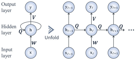
Figure 1. A schematic of a recurrent neutral network and its unfolded structure.

In this work, we use a one-hidden-layer RNN described by the following form as a surrogate model for Equation (1):

$$\begin{array}{cc}\hfill {\mathbf{h}}_{t,\ell }& ={\sigma }_h\left(Q{\mathbf{h}}_{t,\ell -1}+W{\mathbf{x}}_{t,\ell }\right)\hfill \\ \hfill {\mathbf{y}}_{t,\ell }& ={\sigma }_y\left(V{\mathbf{h}}_{t,\ell }\right)\hfill \end{array}$$

(3)

where ${\mathbf{y}}_{t,\ell }\in {\mathbb{R}}^{d_y}$, ${\mathbf{x}}_{t,\ell }\in {\mathbb{R}}^{d_x}$, and ${\mathbf{h}}_{t,\ell }\in {\mathbb{R}}^{d_h}$, $t=1,\dots ,T$ (T is the data sequences) and $\ell =1,\dots ,L_{nn}$ ($L_{nn}$ is the time length), are the RNN outputs, the RNN inputs, and the hidden states, respectively. The weight matrices $V\in {\mathbb{R}}^{d_y\times d_h}$, $Q\in {\mathbb{R}}^{d_h\times d_h}$, and $W\in {\mathbb{R}}^{d_h\times d_x}$ are associated with the output layer, the hidden layer, and the input layer, respectively. The non-linear activation functions ${\sigma }_y$ and ${\sigma }_h$ are associated with the output and the hidden layers, respectively. In this work, we follow the method in [37] to generate historical data for developing the initial offline-learning RNN. Specifically, numerous open-loop simulations are carried out for Equation (1) without disturbances operating under mode k with various conditions $x\in {\Omega }_{{\rho }_k}$ and $u_k\in U_k$, where $u_k$ is applied to the system of Equation (1) in a sample-and-hold fashion at each sampling step (i.e., $u_k\left(t\right)=u_k\left(t_q\right)$ holds for $t\in$$\left[t_q,t_{q+1}\right)$, $t_{q+1}:=t_q+\Delta$, where $\Delta$ is the sampling period). Subsequently, the initial RNN model is developed with open-loop simulation data to predict one sampling period forward using $\mathbf{x}=\left[x\left(t_q\right)u_k\left(t_q\right)\right]$ as RNN inputs. The RNN outputs $\mathbf{y}$ are the predicted states within one sampling period (i.e., $t\in [t_q,t_{q+1})$) that contain all internal time steps of $L_{nn}=\Delta /{\overline{h}}_c$, where ${\overline{h}}_c$ denotes the integration time step with a sufficiently small value used for solving the system of Equation (1) with numerical methods (e.g., the explicit Euler method). Without loss of generality, RNNs are developed under the following assumptions [38]:

Assumption 1. 

An upper bound exists for the RNN inputs in the sense that for all $t=1,\dots ,T$, $\left|{\mathbf{x}}_{t,\ell }\right|\le B_X$, where $\ell =1,\dots ,L_{nn}$.

Assumption 2. 

There are upper bounds for the weight matrices in the sense that ${\parallel V\parallel }_F\le B_{V,F}$, ${\parallel Q\parallel }_F\le B_{Q,F}$, and ${\parallel W\parallel }_F\le B_{W,F}$.

Assumption 3. 

${\sigma }_y$ is a positive-homogeneous and 1-Lipschitz continuous activation function in the sense that for all $\beta \ge 0$, ${\sigma }_y\left(\beta z\right)=\beta {\sigma }_y\left(z\right)$, where $z\in \mathbb{R}$.

Let $h(·)\in \mathcal{H}$ be the RNN model mapping the RNN input to the RNN output ($\mathbf{x}\to \mathbf{y}$), where $\mathcal{H}$ denotes the hypothesis class. In this work, we use the mean squared error (MSE) as the loss function $L(h\left(\mathbf{x}),\overline{\mathbf{y}}\right)$ for the development of RNNs, where $\overline{\mathbf{y}}\in {\mathbb{R}}^{d_y}$ represents the true or labeled output vector. Since the training dataset for RNNs is generated for bounded states $x\in {\Omega }_{{\rho }_k}$ and inputs $u_k\in U_k$, there is an upper bound (denoted by $r_{\ell }$) for the RNN output ${\mathbf{y}}_{\ell }$ and the true output ${\overline{\mathbf{y}}}_{\ell }$, i.e., $|{\overline{\mathbf{y}}}_{\ell }|,|{\mathbf{y}}_{\ell }|\le r_{\ell }$ for $\ell =1,\dots ,L_{nn}$, where $r_{\ell }>0$. Therefore, the MSE loss function meets the local Lipschitz property in the sense that for all $|{\mathbf{y}}_{\ell }|,|{\overline{\mathbf{y}}}_{\ell }|\le r_{\ell }$, the inequality $\left|L\left({\mathbf{y}}_{\ell }^{\prime },\overline{{\mathbf{y}}_{\ell }}\right)-L\left({\mathbf{y}}_{\ell },\overline{{\mathbf{y}}_{\ell }}\right)\right|\le L_r\left|{\mathbf{y}}_{\ell }^{\prime }-{\mathbf{y}}_{\ell }\right|$ is satisfied, where $L_r$ represents the local Lipschitz constant.

3. Online Learning of RNNs

Offline-trained RNNs are constructed based on historical data gathered from Equation (1) without disturbances, and may not be capable of capturing the dynamics of Equation (1) in real-time operation involving disturbances. Therefore, online learning is applied to update ML models to approximate the non-linear dynamics of Equation (1) with disturbances using real-time data. To integrate online ML models with EMPC for switched non-linear systems, ML models need to be developed with the desired predictive capacity on unseen testing data, which is commonly measured by generalized error bounds. In this section, the generalized error bounds for RNN models updated online using i.i.d. and non-i.i.d. training data points are developed, respectively.

3.1. Generalized Error of RNNs Updated Online with i.i.d. Training Data

We first consider a special case of switched non-linear systems, where the system dynamics of Equation (1) does not vary over time, and, thus, Equation (1) can be simplified to the following state-space model:

$$\dot{x}=F(x,u):=f\left(x\right)+g\left(x\right)u$$

(4)

It is assumed that there exist multiple steady-states $x_{s_k}$ for the non-linear system of Equation (4) under the stabilizing controller $u=u_s$, where $k\in \psi =\{1,2,\dots ,p\}$ and $p>1$ is a positive integer that represents the number of steady-states. When Equation (4) operates within the stability region around the steady-state $x_{s_k}$, $k\in \psi$, $\forall t\in \left[t_k^{in},t_k^{out}\right)$, we define the system operating in mode k. In this section, we assume that historical data are only available for a portion of the stability region around $x_{s_k}$. The initial RNN developed with the limited historical data around $x_{s_k}$ may not be capable of approximating the system dynamics of Equation (4) when the system operates in the stability region around another steady-state (e.g., $x_{s_f}$, $f\in \psi$). Therefore, it is essential to update the RNN models with improved prediction accuracy through online learning. In this case, online learning RNNs are developed using real-time process data that are drawn i.i.d. from the system of Equation (4).

We consider a sequence of data samples $(X_1,Y_1)$, …, $(X_T,Y_T)$ drawn i.i.d. from the same distribution $\mathcal{D}$ (e.g., the system of Equation (1)), where the online update of ML models takes place sequentially by processing these i.i.d. samples. Specifically, given an initial hypothesis $h_1\in \mathcal{H}$, the online learner $\mathcal{A}$ receives an instance $X_t$ and makes a prediction $h_t\left(X_t\right)$ on the t-th round, where $t=1,\dots ,T$. Subsequently, the learner $\mathcal{A}$ receives the true output $Y_t$, incurs the loss $L(h_t\left(X_t\right),Y_t)$ (e.g., the MSE loss), and then updates the ML model from $h_t$ to $h_{t+1}$ after processing $(X_t,Y_t)$. Therefore, the learner $\mathcal{A}$ yields $h_1,h_2\dots ,h_{T+1}$ (i.e., a sequence of hypotheses) after T rounds. To simplify the notation, the loss $L(h_t\left(X_t\right),Y_t)$ is denoted by $L(h_t,Z_t)$ for any data sample $Z_t=(X_t,Y_t)$, and we use the shorthand ${\mathbf{Z}}_n^m$ to represent $Z_n,Z_{n+1},\dots ,Z_m$ (i.e., a sequence of data samples). In general, the goal of the online learner $\mathcal{A}$ is to minimize the regret after the end of T rounds, which is defined as follows [32]:

$$\begin{array}{c}\hfill {Reg}_{\mathcal{A}}\left(T\right)=\sum _{t=1}^{T}L\left(h_t,Z_t\right)-\sum _{t=1}^{T}L\left(h^{\star },Z_t\right)\end{array}$$

(5)

where the first term denotes the cumulative loss of hypotheses $h_1,\dots ,h_T$, and the second term represents the minimum cumulative loss that is achieved by the best mode $h^{\star }$ in the hypothesis class $\mathcal{H}$, where $h^{\star }$ is defined by: $h^{\star }=\underset{h\in \mathcal{H}}{argmin}{\sum }_{t=1}^{T}L\left(h,Z_t\right)$. Note that we can only obtain $h^{\star }$ in hindsight after the learner receives all the samples ${\mathbf{Z}}_1^T$. Given a hypothesis h, its generalized error is defined as the expected loss at a new data point $(X,Y)$: $R\left(h\right)=\mathbb{E}\left[L\left(h\left(X\right),Y\right)\right]$.

The following lemma gives the generalized error bound for an ensemble hypothesis of ML models updated online using i.i.d. training set.

Lemma 1 

([34]). Given the training set ${\mathbf{Z}}_1^T$ drawn i.i.d. from the same distribution $\mathcal{D}$, the learner $\mathcal{A}$ produces the hypotheses $h_1,\dots ,h_T$ by processing the samples ${\mathbf{Z}}_1^T$ sequentially with the loss function $L(·,·)$ that is convex in its first argument and satisfies $0\le L(·,·)\le M$. Let ${\Omega }_T=:\left\{\lambda \in {\mathbb{R}}^T\mid {\lambda }_t\ge 0\forall t=1,\dots ,T,\mathrm{and}{\sum }_{t=1}^T{\lambda }_t=1\right\}$ be a unit simplex, $\lambda =({\lambda }_1\dots {\lambda }_T)\in {\Omega }_T$ be a weight vector, and $h={\sum }_{t=1}^T{\lambda }_t{h}_t$ be the ensemble hypothesis. Then, with a probability no less than $1-\delta$, the following inequalities are satisfied for any $\delta >0$:

$$\begin{array}{cc}\hfill & R\left(h\right)\le M\left|\lambda \right|\sqrt{2log\frac{1}{\delta }}+\sum _{t=1}^T{\lambda }_{t}L\left(h_t,Z_t\right)\hfill \end{array}$$

(6)

$$\begin{array}{cc}\hfill & R\left(h\right)\le M\left|\lambda \right|\sqrt{2log\frac{1}{\delta }}+\sum _{t=1}^{T}M|{\lambda }_t-\frac{1}{T}|+\sum _{t=1}^T{\lambda }_{t}L\left(h^{\star },Z_t\right)+\frac{{Reg}_{\mathcal{A}}\left(T\right)}{T}\hfill \end{array}$$

(7)

The generalized error bound for $h={\sum }_{t=1}^T{\lambda }_t{h}_t$ given by the right-hand side (RHS) of Equation (6) depends on the cumulative loss incurred by the online algorithm after T rounds (the second term) and an error function (the first term) with respect to some parameters $\lambda$, $\delta$, and M that represent the weight vector, the confidence level, and the upper bound for $L(·,·)$, respectively. Additionally, Equation (7) is derived using online-to-batch conversion to establish an important connection between the generalized error in the batch setting and the regret of an online learning algorithm. In detail, the generalized error $R\left(h\right)$ is bounded by two error functions based on T, $\lambda$, M, and $\delta$, the cumulative loss of $h^{\star }$, and the average regret in T rounds. The average regret converges to zero if the online algorithm $\mathcal{A}$ achieves a sub-linear regret bound (i.e., ${Reg}_{\mathcal{A}}\left(T\right)=\mathcal{O}\left(\sqrt{T}\right)$), and the two error functions are known once the parameters of $\delta$ and $\lambda$ are chosen. Finally, it is noted that the weight vector $\lambda$ is a dominant factor that affects the calculation of the generalized error bound in Lemma 1. Therefore, to achieve a low generalized error, the weight vector $\lambda$ for the hypotheses $h_1,\dots ,h_T$ can be optimized by solving the optimization problem as follows [34]:

$$\underset{\lambda \in {\Omega }_T}{min}\sum _{t=1}^T{\lambda }_{t}L\left(h_t,Z_t\right)s.t.\sum _{t=1}^T|{\lambda }_t-\frac{1}{T}|\le \alpha$$

(8)

where the objective function is the cumulative loss of hypotheses $h_1,\dots ,h_T$, ${\sum }_{t=1}^T|{\lambda }_t-\frac{1}{T}|\le \alpha$ is an inequality constraint used for constraining the difference between the weight ${\lambda }_t$ and $1/T$, and $\alpha \ge 0$ denotes a hyperparameter predetermined by a validation procedure.

3.2. Generalized Error of RNNs Updated Online with Non-i.i.d. Training Set

We next consider the switched non-linear systems of Equation (1) subject to bounded disturbances and the system is switched between different modes with time-varying system dynamics. As a result, process data collected in real-time operation of the system of Equation (1) are non-i.i.d. samples. The notations and the training procedure of RNNs updated with non-i.i.d. training samples follow those in the i.i.d. case. The only difference is that $(X_{T+1},Y_{T+1})$ (i.e., the new data point) in the non-i.i.d. setting is conditioned on the past samples ${\mathbf{Z}}_1^T$, and thus, the generalized error of the hypothesis $h\in \mathcal{H}$ is defined as follows [33]:

$$R_{T+1}\left(h,{\mathbf{Z}}_1^T\right):=\mathbb{E}\left[L\left(h\left(X_{T+1}\right),Y_{T+1}\right)\mid {\mathbf{Z}}_1^T\right]$$

(9)

The following lemma provides the generalized error bound for an ensemble hypothesis of ML models updated online using non-i.i.d. training set.

Lemma 2 

([33]). Given the non-i.i.d. training set ${\mathbf{Z}}_1^T$, the learner $\mathcal{A}$ yields hypotheses $h_1,\dots ,h_{T+1}$ by processing samples ${\mathbf{Z}}_1^T$ sequentially. Let the weight vector λ and the loss function $L(·,·)$ be defined in Lemma 1, and $h={\sum }_{t=1}^T{\lambda }_t{h}_{t+1}$ be the ensemble hypothesis. Then, with probability no less than $1-\delta$, the following inequalities are satisfied for any $\delta >0$:

$$R_{T+1}\left(h,{\mathbf{Z}}_1^T\right)\le M\left|\lambda \right|\sqrt{2log\frac{1}{\delta }}+\sum _{t=1}^T{\lambda }_{t}L\left(h_{t+1},Z_{t+1}\right)+disc\left(\lambda \right)$$

(10)

$$R_{T+1}\left(h,{\mathbf{Z}}_1^T\right)\le M\left|\lambda \right|\sqrt{2log\frac{1}{\delta }}+\sum _{t=1}^{T}M|{\lambda }_t-\frac{1}{T}|+\sum _{t=1}^T{\lambda }_{t}L\left(h^{\star },Z_{t+1}\right)+\frac{{Reg}_{\mathcal{A}}\left(T\right)}{T}+disc\left(\lambda \right)$$

(11)

In contrast to the generalized error bound for ML models updated online using i.i.d. training set in Lemma 1, Lemma 2 contains the term $disc\left(\lambda \right)$ in the non-i.i.d. case, which is used to quantify the divergence of the sample and target distributions, and is given by [33]:

$$disc\left(\lambda \right)=\underset{h_t\in \mathcal{H}}{sup}\left|\sum _{t=1}^T{\lambda }_t\left(R_{t+1}\left(h_{t+1},{\mathbf{Z}}_1^t\right)-R_{T+1}\left(h_{t+1},{\mathbf{Z}}_1^T\right)\right)\right|$$

(12)

Since the calculation of $disc\left(\lambda \right)$ requires knowledge of the distribution of $Z_{T+1}$ and we do not have access to $Z_{T+1}$ at the end of the T-th round, the discrepancy $disc\left(\lambda \right)$ needs to be estimated based on the given data samples. Based on the results of Theorem 2 in [39] and Lemma 7 in [33], showing that the discrepancy $disc\left(\lambda \right)$ can be bounded using sequential Rademacher complexity, the following lemma presents the generalized error bound for ML models updated online using non-i.i.d. training set in terms of sequential Rademacher complexity.

Lemma 3 

([35]). Given the non-i.i.d. training set ${\mathbf{Z}}_1^T$, let $h={\sum }_{t=1}^T{\lambda }_t{h}_{t+1}$ be the ensemble hypothesis that is developed satisfying all the conditions in Lemma 2. Consider a family of loss functions $\mathcal{F}$ defined by $\mathcal{F}:=\left\{(\mathbf{x},\overline{\mathbf{y}})\to L(h\left(\mathbf{x}\right),\overline{\mathbf{y}}),h\in \mathcal{H}\right\}$. For any $\delta >0$, the following inequality is satisfied with probability no less than $1-\delta$:

$$\begin{array}{cc}\hfill R_{T+1}\left(h,{\mathbf{Z}}_1^T\right)\le & 2M\left|\lambda \right|\sqrt{2log\frac{1}{\delta }}+\sum _{t=1}^T{\lambda }_{t}L\left(h_{t+1},Z_{t+1}\right)+\left|\lambda \right|+\Lambda +{\widehat{disc}}_{\mathcal{H}}\left(\lambda \right)\hfill \\ \hfill & +6\sqrt{logT\pi }M{\mathcal{R}}_T^{seq}\left(\mathcal{F}\right)\hfill \end{array}$$

(13)

where ${\widehat{disc}}_{\mathcal{H}}\left(\lambda \right):={sup}_{\overline{h},h_t\in \mathcal{H}}\left|{\sum }_{t=1}^T{\lambda }_t\left(L\left(h_{t+1},Z_{t+1}\right)-L\left(h_{t+1}\left(X_{T+1}\right),\overline{h}\left(X_{T+1}\right)\right)\right)\right|$ denotes the empirical discrepancy, $\Lambda :={inf}_{{\overline{h}}^{\star }\in \mathcal{H}}\mathbb{E}\left[\left(L_r\left|{\overline{h}}^{\star }\left(X_{T+1}\right)-Z_{T+1}\right|\right)\mid {\mathbf{Z}}_1^T\right]$, and ${\mathcal{R}}_T^{seq}\left(\mathcal{F}\right)$ denotes the sequential Rademacher complexity of the function class $\mathcal{F}$.

It is noted that $\Lambda$ and ${\widehat{disc}}_{\mathcal{H}}\left(\mathbf{\lambda }\right)$ can be computed and optimized based on the given data samples, and $\left|\mathbf{\lambda }\right|$ can be obtained once the weight vector $\mathbf{\lambda }$ is chosen. As a result, to calculate the generalized error bound of Equation (13), it remains to characterize the upper bound on ${\mathcal{R}}_T^{seq}\left(\mathcal{F}\right)$. The definition of sequential Rademacher complexity is given below.

Definition 1. 

(Sequential Rademacher complexity [33]). Let $\mathbf{z}$ be a $\mathcal{Z}$-valued, T-depth tree and $\mathcal{G}$ be a class of functions mapping $\mathcal{Z}\to \mathbb{R}$. The sequential Rademacher complexity of a function class $\mathcal{G}$ on a $\mathcal{Z}$-valued tree $\mathbf{z}$ is given by:

$${\mathcal{R}}_T^{seq}\left(\mathcal{G}\right)=\underset{\mathbf{z}}{sup}\mathbb{E}\left[\underset{g\in \mathcal{G}}{sup}\sum _{t=1}^T{\lambda }_t{ϵ}_{t}g\left(z_t\left(\mathbf{ϵ}\right)\right)\right]$$

(14)

where $ϵ=\left({ϵ}_1,\dots ,{ϵ}_{T-1}\right)$ represents a set of Rademacher random variables drawn i.i.d. from $\{-1,1\}$ and $z_t\left(\mathbf{ϵ}\right)$ denotes $z_t({ϵ}_1,{ϵ}_2,\dots ,{ϵ}_{t-1})$.

Lemma 3 characterizes the generalized error bound for a broad class of online ML models. In the remainder of this section, we will develop the generalized error bound for the RNN model of Equation (3) updated online with non-i.i.d. training set drawn from the non-linear system of Equation (1). We consider the RNN hypothesis class ${\mathcal{H}}_{\ell }$ that maps the first ℓ-time-step inputs to the ℓ-th output, $\ell =1,\dots ,L_{nn}$, and a family of loss functions ${\mathcal{F}}_{\ell }$ associated with ${\mathcal{H}}_{\ell }$ is defined by ${\mathcal{F}}_{\ell }:=\left\{(\mathbf{x},\overline{\mathbf{y}})\to L(h\left(\mathbf{x}\right),\overline{\mathbf{y}}),h\in {\mathcal{H}}_{\ell }\right\}.$ Note that ${\mathcal{H}}_{\ell }$ is a family of vector-valued functions since the RNN model of Equation (3) is developed to approximate the dynamics of the multiple-input and multiple-output non-linear system (i.e., Equation (1)). Following the results of Lemma 4 in [32], we have the following upper bound for ${\mathcal{R}}_T^{seq}\left({\mathcal{F}}_{\ell }\right)$:

$${\mathcal{R}}_T^{seq}\left({\mathcal{F}}_{\ell }\right)\le 8L_r\left(4\sqrt{2}{log}^{3/2}\left(e{T}^2\right)+1\right)\sum _{j=1}^{d_y}{\mathcal{R}}_T^{seq}\left({\mathcal{H}}_{j,\ell }\right)$$

(15)

where ${\mathcal{H}}_{j,\ell }$ denotes a family of real-valued functions that corresponds to the j-th component of ${\mathcal{H}}_{\ell }$, $j=1,\dots ,d_y$, and $d_y$ represents the RNN output dimension. Subsequently, we develop the upper bound on ${\mathcal{R}}_T^{seq}\left({\mathcal{H}}_{j,\ell }\right)$ following the proof techniques in [38] that peel off the weight matrices (i.e., V, W, and Q) and the activation functions (i.e., ${\sigma }_y$ and ${\sigma }_h$) layer by layer.

Lemma 4 

([35]). Consider a family of real-valued functions ${\mathcal{H}}_{j,\ell }$ that corresponds to the j-th component of the RNN hypothesis class ${\mathcal{H}}_{\ell }$, with weight matrices and activation functions that satisfy Assumptions 1–3. The following inequality is satisfied for the RNNs developed with the non-i.i.d. training set ${\mathbf{Z}}_1^T$:

$${\mathcal{R}}_T^{seq}\left({\mathcal{H}}_{j,\ell }\right)\le \left(1+\sqrt{2(\ell +1)log\left(2\right)}\right)\Gamma B_X\left|\lambda \right|$$

(16)

where $\Gamma =\frac{{\left(B_{Q,F}\right)}^{\ell }-1}{B_{Q,F}-1}{B}_{W,F}{B}_{V,F}$.

Based on Equations (13), (15) and (16), the following theorem develops the generalized error bound for RNN models updated online using the non-i.i.d. training set.

Theorem 1  

([35]). Let ${\mathcal{H}}_{\ell }$ be the RNN hypothesis class that maps the first ℓ-time-step inputs to the ℓ-th output, $\ell =1,\dots ,L_{nn}$, $h_1,\dots ,h_{T+1}$ be the hypotheses from ${\mathcal{H}}_{\ell }$ that are developed using the non-i.i.d. training set ${\mathbf{Z}}_1^T$ and meet all the conditions in Lemmas 2–4, and $h={\sum }_{t=1}^T{\lambda }_t{h}_{t+1}$ be the ensemble hypothesis. For any $\delta >0$, the following inequality holds with probability no less than $1-\delta$:

$$\begin{array}{cc}\hfill R_{T+1}\left(h,{\mathbf{Z}}_1^T\right)\le & 2M\left|\mathbf{\lambda }\right|\sqrt{2log\frac{1}{\delta }}+\sum _{t=1}^T{\lambda }_{t}L\left(h_{t+1},Z_{t+1}\right)+\left|\mathbf{\lambda }\right|+\Lambda +{\widehat{disc}}_{\mathcal{H}}\left(\mathbf{\lambda }\right)\hfill \\ & +M{L}_r{C}_T{d}_y\left(1+\sqrt{2(\ell +1)log\left(2\right)}\right)\Gamma B_X\left|\mathbf{\lambda }\right|\hfill \end{array}$$

(17)

where $C_T=\mathcal{O}\left(\sqrt{logT\pi }\left(4\sqrt{2}{log}^{3/2}\left(e{T}^2\right)+1\right)\right)$.

The weight vector $\mathbf{\lambda }$ for the hypotheses $h_1,\dots ,h_{T+1}$ developed with non-i.i.d. training set can be optimized as follows [35]:

$$\begin{array}{c}\hfill \underset{\lambda \in {\Omega }_T}{min}{\widehat{disc}}_{\mathcal{H}}\left(\lambda \right)+\sum _{t=1}^T{\lambda }_{t}L\left(h_{t+1},Z_{t+1}\right)s.t.{\lambda }_T=0,\sum _{t=1}^T|{\lambda }_t-\frac{1}{T}|\le \alpha \end{array}$$

(18)

Remark 1. 

Compared to the optimization problem of Equation (8) for the i.i.d. case, the objective function of Equation (18) accounts for the empirical discrepancy term ${\widehat{disc}}_{\mathcal{H}}\left(\lambda \right)$ for non-i.i.d training set. Additionally, since the cost function of Equation (18) is based on the sample $Z_{T+1}$ that is unavailable after the T-th round, Equation (18) includes an additional equality constraint that lets ${\lambda }_T=0$, and, therefore, $h_{T+1}$ (i.e., the last hypothesis) is discarded. This is consistent with the i.i.d. case where the ensemble hypothesis is developed using the hypotheses $h_1,\dots ,h_T$ without $h_{T+1}$. It should be noted that the initial hypothesis $h_1$ is also discarded for the ensemble hypothesis in the non-i.i.d. case, since $h_1$ is trained offline using historical data that cannot predict the system dynamics of Equation (1) well with disturbances. Therefore, the ensemble hypothesis h is derived using the hypotheses $h_2,\dots ,h_T$, that is, $h={\sum }_{t=1}^{T-1}{\lambda }_t{h}_{t+1}$.

4. RNN-Based LEMPC of Switched Non-Linear Systems

In this section, we develop a framework that integrates online learning RNN models with Lyapunov-based EMPC (RNN-LEMPC) for switched non-linear systems. Specifically, for each switching mode $k\in \psi$, the closed-loop state of Equation (1) is maintained in the prescribed stability region while an economic cost function is maximized to obtain optimal economic performance for the system under RNN-LEMPC. Additionally, due to the switching behavior of Equation (1), an appropriate mode transition constraint is included in the RNN-LEMPC formulation to guarantee the success of scheduled mode transitions. Note that in this section, we will only discuss the case of RNNs updated online with non-i.i.d. training set for modeling Equation (1) involving process disturbances, since Equation (4) switched between different steady-states without disturbances (the i.i.d. case) is a special case of Equation (1) and the stability results derived in this section can be easily adapted to the i.i.d. case.

4.1. Lyapunov-Based Control Using RNN Models

To simplify the closed-loop stability analysis for the system of Equation (1) under RNN-LEMPC, we represent the RNN model of Equation (3) in the following continuous-time state-space form:

$$\dot{\widehat{x}}=F_{{nn}_k}(\widehat{x},u_k)$$

(19)

where $\widehat{x}\in {\mathbb{R}}^n$ denotes the RNN state vector and $u_k\in {\mathbb{R}}^{n_u}$ represents the control input vector. For each mode $k\in \psi$, a stabilizing control law $u_k={\Phi }_{{nn}_k}\left(x\right)\in U_k$ is assumed to exist in the sense that the origin of the RNN of Equation (19) is rendered exponentially stable. This stabilizability assumption indicates that there is a control Lyapunov function ${\widehat{V}}_k\left(x\right)$ belonging to class ${\mathcal{C}}^1$ such that the following inequalities are satisfied for all states x in ${\widehat{D}}_k$:

$$\begin{array}{c}{\widehat{c}}_{1_k}{\left|x\right|}^2\le {\widehat{V}}_k\left(x\right)\le {\widehat{c}}_{2_k}{\left|x\right|}^2,\end{array}$$

(20a)

$$\begin{array}{c}\frac{\partial {\widehat{V}}_k\left(x\right)}{\partial x}{F}_{{nn}_k}(x,{\Phi }_{{nn}_k}\left(x\right))\le -{\widehat{c}}_{3_k}{\left|x\right|}^2,\end{array}$$

(20b)

$$\begin{array}{c}\left|\frac{\partial {\widehat{V}}_k\left(x\right)}{\partial x}\right|\le {\widehat{c}}_{4_k}\left|x\right|,\end{array}$$

(20c)

where ${\widehat{D}}_k$ denotes an open neighborhood around the origin, ${\widehat{c}}_{i_k},i=1,2,3,4$, $k\in \psi$, are positive constants. Similarly to the construction procedure of the stability region for Equation (1) without disturbances, the stability region for the RNN model of Equation (19) operating under mode k with $u_k={\Phi }_{{nn}_k}\left(x\right)\in U_k$ is characterized as a level set of ${\widehat{V}}_k\left(x\right)$ as follows: ${\Omega }_{{\widehat{\rho }}_k}:=\left\{x\in {\mathbb{R}}^n\mid {\widehat{V}}_k\left(x\right)\le {\widehat{\rho }}_k\right\}$, where ${\widehat{\rho }}_k>0$ for $k\in \psi$. Historical data are assumed to be available for Equation (1) without disturbances operating under each mode $k\in \psi$, and, thus, the initial RNN can be constructed offline using the corresponding historical data to approximate the nominal system dynamics for each mode, respectively. Subsequently, ${\Phi }_{{nn}_k}\left(x\right)$ and ${\Omega }_{{\widehat{\rho }}_k}$ for the initial RNN model can be characterized accordingly. Note that although the online update of RNNs is carried out using real-time data in this work, ${\Omega }_{{\widehat{\rho }}_k}$ and ${\Phi }_{{nn}_k}\left(x\right)$ will not be updated accordingly due to the excessive computational burden of real-time characterization of ${\Omega }_{{\widehat{\rho }}_k}$ and ${\Phi }_{{nn}_k}\left(x\right)$ for online learning RNNs. Therefore, ${\Phi }_{{nn}_k}\left(x\right)$ and ${\Omega }_{{\widehat{\rho }}_k}$ designed using the initial RNN remain unchanged at all times, and we will demonstrate that closed-loop stability for Equation (1) in terms of the boundedness of the state within the stability region is achieved in probability under LEMPC using online learning RNNs.

4.2. Lyapunov-Based EMPC Using RNN Models

Before we proceed to the closed-loop stability analysis for the system of Equation (1) under RNN-LEMPC, we need the following propositions that guarantee closed-loop stability of the system of Equation (1) under the controller $u_k={\Phi }_{{nn}_k}\left(x\right)\in U_k$. Specifically, Proposition 1 derives an upper bound for the state error between the RNN predicted state $\widehat{x}\left(t\right)$ of Equation (19) and the actual state $x\left(t\right)$ of Equation (1) taking into account bounded disturbances and model mismatch.

Proposition 1 

([40]). Consider the RNN model of Equation (19) and the system of Equation (1) operating in mode k with the same initial condition ${\widehat{x}}_0=x_0\in {\Omega }_{{\widehat{\rho }}_k}$, $t_k^{out}=\infty$, and $|w_k|\le w_{m_k}$. There exist a function $f_k(·)$ belonging to class $\mathcal{K}$ and a positive constant κ such that for all $x,\widehat{x}\in {\Omega }_{{\widehat{\rho }}_k}$, the following inequalities hold with probability no less than $1-\delta$:

$$\begin{array}{c}|x\left(t\right)-\widehat{x}\left(t\right)|\le f_k\left(t\right):=\frac{E_I+L_{w_k}{w}_{m_k}}{L_{x_k}}(e^{L_{x_k}t}-1)\end{array}$$

(21a)

$$\begin{array}{c}{\widehat{V}}_k\left(x\right)\le \kappa |x-\widehat{x}{|}^2+\frac{{\widehat{c}}_{4_k}\sqrt{{\widehat{\rho }}_k}}{\sqrt{{\widehat{c}}_{1_k}}}|x-\widehat{x}|+{\widehat{V}}_k\left(\widehat{x}\right)\end{array}$$

(21b)

where $E_I$ denotes an upper bound for the model mismatch between the initial RNN model of Equation (19) and the system of Equation (1) without disturbances (i.e., $|F_{{nn}_k}(x,u_k))-F_k(x,u_k,0)|\le E_I$). The formulation of $E_I$ can be derived using the generalized error bound for offline-trained RNNs (see [38] for details).

Remark 2. 

Since the initial RNN can capture the nominal system dynamics only, Equation (21a) is derived by taking $w_k=w_{m_k}$ (i.e., the worst-case scenario) into consideration. However, in this work, RNNs are iteratively updated using real-time data to capture non-linear dynamics of Equation (1) subject to bounded disturbances, such that the modeling error between the online learning RNN models of Equation (19) and the system of Equation (1) is bounded by the modeling error bound $E_O$ with probability no less than $1-\delta$, i.e., $|F_{{nn}_k}(x,u_k)-F_k(x,u_k,w_k)|\le E_O$. Based on the generalized error bound $E_P$ for RNNs updated online with non-i.i.d. training set (i.e., $E_P$ is given by the RHS of Equation (17)), the finite difference method can be used to approximate the modeling error bound $E_O$. Note that the inequality $|x-\widehat{x}|\le \sqrt{E_P}$ holds with probability no less than $1-\delta$ if the MSE loss function is utilized in this work. Similarly to the derivation of Equation (21a), the following inequality holds with probability no less than $1-\delta$:

$$|x\left(t\right)-\widehat{x}\left(t\right)|\le f_k\left(t\right):=\frac{E_O}{L_{x_k}}(e^{L_{x_k}t}-1)$$

(22)

In contrast to Equation (21a), it is readily seen from Equation (22) that if the RNNs are updated well, such that the inequality $E_O\le L_{w_k}{w}_{m_k}+E_I$ is satisfied, the state error $|x\left(t\right)-\widehat{x}\left(t\right)|$ achieved by the online learning RNN is smaller compared to that of the initial RNN trained offline.

Proposition 2 below demonstrates that if the initial RNN is trained to model the nominal system well (i.e., $|F_{{nn}_k}(x,u_k))-F_k(x,u_k,0)|$ is sufficiently small), the closed-loop state of Equation (1) can be driven towards the origin and bounded in the stability region ${\Omega }_{{\widehat{\rho }}_k}$ at all times under $u_k={\Phi }_{{nn}_k}\left(x\right)\in U_k$ applied to the system of Equation (1) in a sample-and-hold fashion.

Proposition 2  

([40]). Consider Equation (1) operating in mode k with $t_k^{out}=\infty$, $|w_k|\le w_{m_k}$, under $u_k={\Phi }_{{nn}_k}\left(x\right)\in U_k$ that is applied in a sample-and-hold fashion and meets the conditions of Equation (20). If the modeling error between the initial RNN model and the system of Equation (1) without disturbances can be bounded by $|F_{{nn}_k}(x,u_k)-F_k(x,u_k,0)|\le E_I\le {\gamma }_k\left|x\right|$, and there exist $0<{\rho }_{s_k}<{\widehat{\rho }}_k$, $\Delta >0$, and ${ϵ}_k>0$, $k\in \psi$, such that the following inequality is satisfied:

$$L_{x_k}^{\prime }{M}_k\Delta +L_{w_k}^{\prime }{w}_{m_k}-\frac{{\tilde{c}}_{3_k}}{{\widehat{c}}_{2_k}}{\rho }_{s_k}\le -{ϵ}_k$$

(23)

where ${\tilde{c}}_{3_k}={\widehat{c}}_{3_k}-{\widehat{c}}_{4_k}{\gamma }_k>0$ for ${\gamma }_k$ satisfying $0<{\gamma }_k<{\widehat{c}}_{3_k}/{\widehat{c}}_{4_k}$, $k\in \psi$, then, with probability no less than $1-\delta$, the following inequality holds for $t\in \left[t_q,t_{q+1}\right)$ and $\forall x\left(t_q\right)\in {\Omega }_{{\widehat{\rho }}_k}\backslash {\Omega }_{{\rho }_{s_k}}$:

$${\widehat{V}}_k\left(x\left(t\right)\right)\le {\widehat{V}}_k\left(x\left(t_q\right)\right)$$

(24)

The following proposition ensures that under $u_k={\Phi }_{{nn}_k}\left(x\right)\in U_k$, the closed-loop state can be driven to the stability region of mode f when the system of Equation (1) is switched to the subsequent mode f from the current mode k at the prescribed switching time.

Proposition 3 

([34]). Consider Equation (1) operating in mode k for $t\in [t_k^{in},t_k^{out})$, with $|w_k|\le w_{m_k}$, and under $u_k={\Phi }_{{nn}_k}\left(x\right)\in U_k$ satisfying the conditions in Proposition 1 and Proposition 2. Given $t_k^{in}\le t<t_k^{out}=t_f^{in}$ and $x\left(t_k^{in}\right)\in {\Omega }_{{\widehat{\rho }}_k}$ for some $f,k\in \psi$, if there exist positive real numbers ${\widehat{\rho }}_k$, Δ, ${ϵ}_k$, and $N_k$, such that

$${\widehat{c}}_{2_f}{\left(\left|x_{s_k}-x_{s_f}\right|+\sqrt{\frac{{\widehat{\rho }}_k-{ϵ}_k{N}_k\Delta }{{\widehat{c}}_{1_k}}}\right)}^2\le {\widehat{\rho }}_f$$

(25)

then $x\left(t_f^{in}\right)\in {\Omega }_{{\widehat{\rho }}_f}$.

The RNN-LEMPC scheme that optimizes economic benefits while maintaining closed-loop stability for Equation (1) is represented by the optimization problem as follows:

$$\begin{array}{cc}\hfill \mathcal{J}=& \underset{u_k\in S(\Delta )}{\max }{\int }_{t_q}^{t_k^{out}}{l}_e(\tilde{x}\left(t\right),u_k\left(t\right))dt\hfill \end{array}$$

(26a)

$$\begin{array}{cc}\hfill \mathrm{s}.\mathrm{t}.& \dot{\tilde{x}}\left(t\right)=F_{{nn}_k}(\tilde{x}\left(t\right),u_k\left(t\right))\hfill \end{array}$$

(26b)

$$\begin{array}{cc}\hfill & \tilde{x}\left(t_q\right)=x\left(t_q\right)\hfill \end{array}$$

(26c)

$$\begin{array}{cc}\hfill & u_k\left(t\right)\in U_k,\forall t\in [t_q,t_k^{out})\hfill \end{array}$$

(26d)

$$\begin{array}{cc}\hfill & {\widehat{V}}_k\left(\tilde{x}\left(t\right)\right)\le {\widehat{\rho }}_{e_k},\forall t\in [t_q,t_k^{out}),ifx\left(t_q\right)\in {\Omega }_{{\widehat{\rho }}_{e_k}}\hfill \end{array}$$

(26e)

$$\begin{array}{cc}\hfill & {\dot{\widehat{V}}}_k(x\left(t_q\right),u_k)\le {\dot{\widehat{V}}}_k(x\left(t_q\right),{\Phi }_{{nn}_k}\left(x\left(t_q\right)\right)),\mathrm{if}x\left(t_q\right)\in {\Omega }_{{\widehat{\rho }}_k}\backslash {\Omega }_{{\widehat{\rho }}_{e_k}}\hfill \end{array}$$

(26f)

$$\begin{array}{cc}\hfill & {\widehat{V}}_f\left(\tilde{x}\left(t_k^{out}\right)\right)+f_e\left(E_P\right)\le {\widehat{\rho }}_f\hfill \end{array}$$

(26g)

where $\tilde{x}\left(t\right)$ and $S(\Delta )$ represent the predicted state trajectory and the class of piecewise constant functions with sampling period $\Delta$, and $f_e\left(E_P\right):=\frac{{\widehat{c}}_{4_k}\sqrt{{\widehat{\rho }}_k}}{\sqrt{{\widehat{c}}_{1_k}}}\sqrt{E_P}+\kappa E_P$ is used to evaluate the impact of $E_P$ (i.e., $|x-\widehat{x}|\le \sqrt{E_P}$) on the Lyapunov function value based on Equation (21b). At the current sampling time step $t_q$, the optimization problem of Equation (26) is solved by maximizing the economic cost function of Equation (26a) over a shrinking prediction horizon for $t\in [t_q$, $t_k^{out}$) and taking into account the constraints of Equations (26b)–(26g). In detail, Equation (26b) represents the prediction model that utilizes the initial RNN at the beginning and then is iteratively updated using real-time data. This prediction model is utilized to forecast future states $\tilde{x}\left(t\right)$ for $t\in [t_q,t_k^{out})$ given $\tilde{x}\left(t_q\right)$ obtained from the state measurement $x\left(t_q\right)$ in Equation (26c). The constraint of Equation (26d) is incorporated to bound the control inputs $u\left(t\right)$ for $t\in [t_q,t_k^{out})$. Additionally, by designing ${\Omega }_{{\widehat{\rho }}_{e_k}}$ as a subset of ${\Omega }_{{\widehat{\rho }}_k}$ (i.e., ${\widehat{\rho }}_{e_k}<{\widehat{\rho }}_k$), the constraints of Equations (26e) and (26f) are designed to ensure that the predicted state $\tilde{x}\left(t\right)$ moves toward ${\Omega }_{{\widehat{\rho }}_{e_k}}$ and remains inside ${\Omega }_{{\widehat{\rho }}_k}$ at all times, and it will be demonstrated in Theorem 2 that the actual state $x\left(t\right)$ of Equation (1) is maintained in ${\Omega }_{{\widehat{\rho }}_k}$. Finally, Equation (26g) is the mode transition constraint used to drive the state $x\left(t\right)$ to ${\Omega }_{{\widehat{\rho }}_f}$ at $t=t_k^{out}$.

It should be pointed out that when the prediction model (i.e., Equation (26b)) is updated online, all the terms in the RNN-LEMPC of Equation (26) associated with the Lyapunov function (i.e., Equation (26e), the LHS of Equation (26f), and Equation (26g)) use the latest RNN model except that the RHS of Equation (26f) utilizes the initial RNN at all times. Since the results of Propositions 1–3 are established under $u_k={\Phi }_{{nn}_k}\left(x\right)\in U_k$ constructed using the initial RNN, the constraints of Equations (26e)–(26g) under $u_k={\Phi }_{{nn}_k}\left(x\right)\in U_k$ may not hold due to the model inconsistency. Therefore, Equation (26) may not be guaranteed to be feasible once the prediction model is updated. To remedy this, the controller ${\Phi }_{{nn}_k}\left(x\right)$ will be utilized for the next sampling period to stabilize the system of Equation (1) as a backup controller in the case of infeasibility of Equation (26) for some sampling steps. Finally, we develop the following theorem to guarantee that the closed-loop state of Equation (1) is maintained in ${\Omega }_{{\widehat{\rho }}_k}$ at all times and is driven into ${\Omega }_{{\widehat{\rho }}_f}$ at the switching moment under the RNN-LEMPC of Equation (26) with updating RNN models.

Theorem 2. 

Consider the system of Equation (1) with $|w_k|\le w_{m_k}$ under the RNN-LEMPC of Equation (26) using ${\Phi }_{{nn}_k}\left(x\right)$ as the backup controller when Equation (26) is infeasible. Let $0<{\rho }_{s_k}<{\widehat{\rho }}_{e_k}<{\widehat{\rho }}_k$, $\Delta >0$, ${ϵ}_k>0$, $k\in \psi$, satisfy

$${\widehat{\rho }}_{e_k}\le -\kappa {\left(f_k(\Delta )\right)}^2-\frac{{\widehat{c}}_{4_k}\sqrt{{\widehat{\rho }}_k}}{\sqrt{{\widehat{c}}_{1_k}}}{f}_k(\Delta )+{\widehat{\rho }}_k$$

(27)

where $f_k(·)$ is defined in Equation (21a) for the initial RNN and Equation (22) for online updating RNNs, respectively. For some $k,f\in \psi$, if $x\left(t_k^{in}\right)\in {\Omega }_{{\widehat{\rho }}_k}$ and all the conditions in Propositions 1–3 are satisfied, and the online updating RNNs are developed, such that $|F_{{nn}_k}(x,u_k)-F_k(x,u_k,w_k)|\le E_O\le {\gamma }_k\left|x\right|$ (i.e., the modeling error constraint) is met, then for each sampling step, with probability no less than $1-\delta$, the state $x\left(t\right)$ of Equation (1) is bounded in ${\Omega }_{{\widehat{\rho }}_k}$ for $t\in [t_k^{in},t_k^{out})$ and is driven to ${\Omega }_{{\widehat{\rho }}_f}$ at $t=t_k^{out}=t_f^{in}$.

Proof. 

The proof consists of two parts. We first consider the case where the optimization problem of Equation (26) is infeasible and the control law $u_k={\Phi }_{{nn}_k}\left(x\right)\in U_k$ is applied. In this case, it is demonstrated in Propositions 1–3 that the controller $u_k={\Phi }_{{nn}_k}\left(x\right)\in U_k$ is able to guarantee the boundedness of the state $x\left(t\right)$ within ${\Omega }_{{\widehat{\rho }}_k}$ and the success of the scheduled model transitions for the non-linear system of Equation (1).

Subsequently, we prove that when there is a feasible solution $u_k^{\star }\left(x\left(t_q\right)\right)$ (i.e., the optimal control action) for the RNN-LEMPC of Equation (26) with online updating RNN models, closed-loop stability for Equation (1) holds as well under $u_k^{\star }\left(x\left(t_q\right)\right)$. In detail, if $x\left(t_q\right)\in {\Omega }_{{\widehat{\rho }}_{e_k}}$, the predicted state $\tilde{x}\left(t\right)$ stays in ${\Omega }_{{\widehat{\rho }}_{e_k}}$ following the constraint of Equation (26e). Then, it follows from Proposition 1 that with probability no less than $1-\delta$, the actual state $x\left(t\right)$ of Equation (1) for $t\in [t_q$, $t_{q+1}$) can be bounded as follows:

$$\begin{array}{cc}\hfill {\widehat{V}}_k\left(x\right)& \le \kappa |x-\tilde{x}{|}^2+\frac{{\widehat{c}}_{4_k}\sqrt{{\widehat{\rho }}_k}}{\sqrt{{\widehat{c}}_{1_k}}}|x-\tilde{x}|+{\widehat{V}}_k\left(\tilde{x}\right)\hfill \\ \hfill & \le \kappa {\left(f_k(\Delta )\right)}^2+\frac{{\widehat{c}}_{4_k}\sqrt{{\widehat{\rho }}_k}}{\sqrt{{\widehat{c}}_{1_k}}}{f}_k(\Delta )+{\widehat{V}}_k\left(\tilde{x}\right)\hfill \end{array}$$

(28)

Since ${\widehat{V}}_k\left(\tilde{x}\right)\le {\widehat{\rho }}_{e_k}$, we obtain ${\widehat{V}}_k\left(x\right)\le {\widehat{\rho }}_k$ if Equation (27) holds, indicating that $x\left(t\right)\in {\Omega }_{{\widehat{\rho }}_k}$ for all $t\in [t_q$, $t_{q+1}$) with probability no less than $1-\delta$. Following the proof technique in [40], if $x\left(t_q\right)\in {\Omega }_{{\widehat{\rho }}_k}\backslash {\Omega }_{{\widehat{\rho }}_{e_k}}$, the time derivative of $\widehat{V}\left(x\left(t\right)\right)$ of Equation (1) for $t\in \left[t_q,t_{q+1}\right)$ can be bounded as $\dot{\widehat{V}}\left(x\left(t\right)\right)\le L_{x_k}^{\prime }{M}_k\Delta +\dot{\widehat{V}}\left(x\left(t_q\right)\right)$ using Equation (2). Note that for any $x\left(t_q\right)\in {\Omega }_{{\widehat{\rho }}_k}\backslash {\Omega }_{{\widehat{\rho }}_{e_k}}$, Equation (26f) is activated such that we can further bound $\dot{\widehat{V}}\left(x\left(t_q\right)\right)$ with probability no less than $1-\delta$ as follows:

$$\begin{array}{cc}\hfill \dot{\widehat{V}}\left(x\left(t_q\right)\right)=& \frac{\partial {\widehat{V}}_k\left(x\left(t_q\right)\right)}{\partial x}\left(F_k\left(x\left(t_q\right),u_k^{\star }\left(x\left(t_q\right)\right),w_k\right)-F_{{nn}_k}(x\left(t_q\right),u_k^{\star }\left(x\left(t_q\right)\right))\right)\hfill \\ \hfill & +\frac{\partial {\widehat{V}}_k\left(x\left(t_q\right)\right)}{\partial x}{F}_{{nn}_k}(x\left(t_q\right),u_k^{\star }\left(x\left(t_q\right)\right))\hfill \\ \hfill \le & {\widehat{c}}_{4_k}\left|x\left(t_q\right)\right|·\left|F_{{nn}_k}(x\left(t_q\right),u_k^{\star }\left(x\left(t_q\right)\right))-F_k\left(x\left(t_q\right),u_k^{\star }\left(x\left(t_q\right)\right),w_k\right)\right|\hfill \\ \hfill & +\frac{\partial {\widehat{V}}_k\left(x\left(t_q\right)\right)}{\partial x}{F}_{{nn}_k}(x\left(t_q\right),{\Phi }_{{nn}_k}\left(x\left(t_q\right)\right))\hfill \\ \hfill \le & {\widehat{c}}_{4_k}{\gamma }_k|x\left(t_q\right){|}^2-{\widehat{c}}_{3_k}{\left|x\left(t_q\right)\right|}^2\hfill \\ \hfill \le & -\frac{{\tilde{c}}_{3_k}}{{\widehat{c}}_{2_k}}{\widehat{\rho }}_{e_k}\hfill \end{array}$$

(29)

where the first inequality of Equation (29) is obtained under the constraints of Equations (26f) and (20c). The second inequality of Equation (29) follows from Equation (20b) and the inequality $|F_{{nn}_k}(x,u_k)-F_k(x,u_k,w_k)|\le E_O\le {\gamma }_k\left|x\right|$ for online updating RNNs. Using Equation (20a) for any state $x\left(t_q\right)\in {\Omega }_{{\widehat{\rho }}_k}\backslash {\Omega }_{{\widehat{\rho }}_{e_k}}$, it follows that the last inequality of Equation (29) holds. Therefore, with probability no less than $1-\delta$, the following inequality for $\dot{\widehat{V}}\left(x\left(t\right)\right)$ holds:

$$\begin{array}{cc}\hfill \dot{\widehat{V}}\left(x\left(t\right)\right)& \le L_{x_k}^{\prime }{M}_k\Delta -\frac{{\tilde{c}}_{3_k}}{{\widehat{c}}_{2_k}}{\widehat{\rho }}_{e_k}\hfill \\ \hfill & <L_{x_k}^{\prime }{M}_k\Delta +L_{w_k}^{\prime }{w}_{m_k}-\frac{{\tilde{c}}_{3_k}}{{\widehat{c}}_{2_k}}{\rho }_{s_k}\hfill \end{array}$$

(30)

Due to $0<{\rho }_{s_k}<{\widehat{\rho }}_{e_k}$ and $0<L_{w_k}^{\prime }{w}_{m_k}$, the second inequality of Equation (30) is derived. Therefore, it is demonstrated in Equation (30) that $\dot{\widehat{V}}\left(x\left(t\right)\right)<0$ holds if the constraint of Equation (23) in Proposition 2 is met. This implies that for any $x\left(t_q\right)\in {\Omega }_{{\widehat{\rho }}_k}\backslash {\Omega }_{{\widehat{\rho }}_{e_k}}$, the value of ${\widehat{V}}_k\left(x\right)$ decreases for $t\in \left[t_q,t_{q+1}\right)$ with probability no less than $1-\delta$ under $u_k^{\star }\left(x\left(t_q\right)\right)$, and, thus, the closed-loop state of Equation (1) can enter into ${\Omega }_{{\widehat{\rho }}_{e_k}}$ within finite sampling steps for a certain probability. Additionally, using Equation (21b) and $|x-\widehat{x}|\le \sqrt{E_P}$, the value of ${\widehat{V}}_f\left(x\left(t_k^{out}\right)\right)$ can be bounded with probability no less than $1-\delta$ as follows:

$$\begin{array}{c}\hfill {\widehat{V}}_f\left(x\left(t_k^{out}\right)\right)\le \kappa E_P+\frac{{\widehat{c}}_{4_k}\sqrt{{\widehat{\rho }}_k}}{\sqrt{{\widehat{c}}_{1_k}}}\sqrt{E_P}+{\widehat{V}}_f\left(\tilde{x}\left(t_k^{out}\right)\right)\end{array}$$

(31)

According to Equation (31), we have ${\widehat{V}}_f\left(x\left(t_k^{out}\right)\right)\le {\widehat{\rho }}_f$ if Equation (26g) is met, which indicates that at $t=t_k^{out}$, the closed-loop state $x\left(t\right)$ can be driven into ${\Omega }_{{\widehat{\rho }}_f}$ in probability.

Therefore, closed-loop stability can be achieved for the system of Equation (1) in probability regardless of the feasibility of Equation (26). This completes the proof of Theorem 2. □

Remark 3. 

The RNN-LEMPC of Equation (26) demonstrates that if the state measurement $x\left(t_q\right)$ at $t=t_q$ is in the region ${\Omega }_{{\widehat{\rho }}_{e_k}}$, the economic cost function is maximized within ${\Omega }_{{\widehat{\rho }}_{e_k}}$; if $x\left(t_q\right)\in {\Omega }_{{\widehat{\rho }}_k}\backslash {\Omega }_{{\widehat{\rho }}_{e_k}}$, the predicted state $\tilde{x}\left(t\right)$ is driven towards ${\Omega }_{{\widehat{\rho }}_{e_k}}$. Additionally, it has been proven in Theorem 2 that the actual state $x\left(t\right)$ of Equation (1) is bounded in the stability region ${\Omega }_{{\widehat{\rho }}_k}$ if $\tilde{x}\left(t\right)$ is maintained in ${\Omega }_{{\widehat{\rho }}_{e_k}}$. Therefore, the region ${\Omega }_{{\widehat{\rho }}_{e_k}}$ is a “safe" operating region in which the RNN-LEMPC of Equation (26) can maximize economic benefits while maintaining the boundedness of the state $x\left(t\right)$ within ${\Omega }_{{\widehat{\rho }}_k}$. It is noted from Equation (27) that the relation between ${\Omega }_{{\widehat{\rho }}_{e_k}}$ and ${\Omega }_{{\widehat{\rho }}_k}$ is determined by $f_k(\Delta )$, which is the upper bound on $|x\left(t\right)-\widehat{x}\left(t\right)|$ within one sampling period Δ. As discussed in Remark 2, online learning RNNs are capable of modeling Equation (1) involving disturbances while the initial RNN can capture the nominal system dynamics only. This implies that compared to the initial model, online learning RNNs may better approximate Equation (1) such that the state error $|x\left(t\right)-\widehat{x}\left(t\right)|$ is smaller, and, thus, a larger ${\widehat{\rho }}_{e_k}$ may be chosen for RNN-LEMPC with online updating RNNs. Therefore, while we use the controller ${\Phi }_{{nn}_k}\left(x\right)$ characterized using the initial offline-trained RNN as a backup controller to stabilize Equation (1) when RNN-LEMPC is infeasible, the online update of RNNs is performed to improve the closed-loop economic performance of Equation (1), which will be illustrated using a non-linear chemical process in the next section.

5. Application to a Chemical Process Example

In this section, a chemical process example is used to illustrate the efficacy of the proposed LEMPC scheme using RNN models updated online. Specifically, a non-isothermal continuous stirred tank reactor (CSTR) is considered, in which a reactant A is transformed into a product B ($A\to B$) via a second-order, irreversible, and exothermic reaction. The CSTR is required to switch between two modes consisting of two available inlet streams with different inlet concentrations $C_{A{0}_{\sigma }}$ and inlet temperatures $T_{0_{\sigma }}$ for the pure reactant A, where $\sigma \in \psi =\{1,2\}$. Additionally, a heating jacket with the heat rate Q is furnished in the CSTR to supply or remove heat for the reactor. At mode $\sigma \in \{1,2\}$, the CSTR dynamic model is described by the following ordinary differential equations:

$$\begin{array}{cc}\hfill & {\displaystyle \frac{d{C}_A}{dt}}=-k_0{e}^{\frac{-E}{RT}}{C}_A^2+{\displaystyle \frac{F}{V}}(C_{A{0}_{\sigma }}-C_A)\hfill \\ \hfill & {\displaystyle \frac{dT}{dt}}={\displaystyle \frac{-\Delta H}{{\rho }_L{C}_p}}{k}_0{e}^{\frac{-E}{RT}}{C}_A^2+{\displaystyle \frac{F}{V}}(T_{0_{\sigma }}-T)+{\displaystyle \frac{Q}{{\rho }_L{C}_{p}V}}\hfill \end{array}$$

(32)

where $C_A$ is the concentration of the reactant A and T is the reactor temperature. A detailed description of the chemical reaction and the process parameters in Equation (32) can be found in [24]. The process parameter values of the CSTR used in the closed-loop simulations are given in Table 1.

Table 1. Parameter values of the CSTR.

$E=5\times {10}^4$ kJ/kmol	$F=5{\mathrm{m}}^3$/h
$R=8.314\mathrm{kJ}/\mathrm{kmol}\mathrm{K}$	$T_{0_1}=300\mathrm{K},T_{0_2}=290$ K
$V=1$ m${}^3$	$Q_s=0.0$ kJ/h
$\Delta H=-1.15\times {10}^4$ kJ/kmol	$C_{A0s_1}$ = 4 kmol/m${}^3$,  $C_{A0s_2}$ = 4.55 kmol/m${}^3$
${\rho }_L=1000$ kg/m${}^3$	$T_{s_1}=402\mathrm{K},T_{s_2}=475$ K
$C_p=0.231$ kJ/kg K	$C_{A{s}_1}$= 1.95 kmol/m${}^3$,  $C_{A{s}_2}$ = 0.83 kmol/m${}^3$
$k_0=8.46\times {10}^6{\mathrm{m}}^3$/kmol h

For each mode, a steady-state $(C_{A{s}_{\sigma }},T_{s_{\sigma }})$ is considered for the CSTR under $\left(C_{A0s_{\sigma }}{Q}_s\right)$ (i.e., the steady-state input values). In this example, two manipulated inputs are the heat input rate Q and the inlet concentration $C_{A{0}_{\sigma }}$, which are denoted by $\Delta Q=Q-Q_s$ and $\Delta C_{A{0}_{\sigma }}=C_{A{0}_{\sigma }}-C_{A0s_{\sigma }}$ in their deviation variable forms, respectively. The manipulated inputs are bounded by $|\Delta Q|\le 5\times {10}^5$ kJ/h and $|\Delta C_{A{0}_{\sigma }}|\le 3.5{\mathrm{kmol}/\mathrm{m}}^3$ for both modes. The input and state vectors in deviation form for the CSTR of Equation (32) are represented by $u^T=[\Delta C_{A{0}_{\sigma }}\Delta Q]$ and $x^T=[C_A-C_{A{s}_{\sigma }}T-T_{s_{\sigma }}]$, respectively, such that the equilibrium point of the CSTR for each mode is at the origin of the steady-space. It is desired to operate the CSTR in ${\Omega }_{{\widehat{\rho }}_{\sigma }}$ (i.e., the stability region) around $(C_{A{s}_{\sigma }},T_{s_{\sigma }})$ while maximizing the production rate of B given by:

$$l_e(x,u)=k_0{e}^{-E/RT}{C}_A^2$$

(33)

The explicit Euler method with a sufficiently small integration time step of ${\overline{h}}_c={10}^{-4}\mathrm{h}$ is applied to numerically solve the CSTR dynamic model of Equation (32). Additionally, the non-linear optimization problem of Equation (26) is solved by PyIpopt [41] with a sampling period of $\Delta ={10}^{-2}\mathrm{h}$.

5.1. The CSTR Switched between Two Modes with Bounded Disturbances

We first consider the CSTR subject to the following disturbances. (1) The upstream disturbance results in the variation of the feed flow rate F in a way that F is time varying and is subject to the constraint: $0\le F\le 5.5{\mathrm{m}}^3/\mathrm{h}$. (2) The catalyst deactivation is considered during process operation; this results in a gradual reduction in the pre-exponential factor $k_0$ that is constrained by: $0\le k_0\le 8.46\times {10}^6{\mathrm{m}}^3/\mathrm{kmol}\mathrm{h}$. Additionally, the control Lyapunov functions for both modes are designed using the quadratic form of $V_{\sigma }\left(x\right)=x^T{P}_{\sigma }x$ with $P_{\sigma }=\left[\begin{array}{cc}1060& 22\\ 22& 0.52\end{array}\right]$ for $\sigma \in \{1,2\}$. As discussed in Section 2.3, we follow the development method of RNN models in [37] to construct two initial RNNs to model the nominal CSTR system (i.e., the values of F and $k_0$ are taken in Table 1 at all times) operating in two modes using historical data gathered from the entire operating region, respectively. Specifically, the RNN models are trained using Keras, where a hidden recurrent layer of 16 neurons is utilized for both initial RNNs, with $tanh$ as the activation function, MSE as the loss function, and Adam as the optimizer. Based on the two initial RNNs, the stability region ${\Omega }_{{\widehat{\rho }}_{\sigma }}$ and a subset ${\Omega }_{{\widehat{\rho }}_{e_{\sigma }}}$ for the CSTR at mode $\sigma \in \{1,2\}$ can be characterized accordingly. In this example, ${\widehat{\rho }}_1$ and ${\widehat{\rho }}_{e_1}$ are chosen to be 368 and 280 for mode 1, and ${\widehat{\rho }}_2$ and ${\widehat{\rho }}_{e_2}$ are chosen to be 228 and 170, respectively. Since the CSTR involves disturbances during process operation, we follow the update strategy in [34] to improve RNN models online to capture the uncertain CSTR system involving bounded disturbances. Specifically, the online update of RNNs is carried out based on the most recent real-time data collected from a fixed time interval (e.g., five sampling periods) and the previous RNN model. The new RNN is utilized to predicate state evolution in LEMPC only if the modeling error constraint in Theorem 2 is met; otherwise, we will discard the new RNN model and use the previous RNN model as the prediction model in LEMPC.

We carry out the closed-loop simulations for the CSTR subject to bounded disturbances and with scheduled mode transitions under RNN-LEMPC as follows. Specifically, the CSTR operates under mode 1 for $t\in [0,0.25$ h) and the mode transition takes place at $t=0.25$ h, after which the CSTR operates under mode 2 for $t\in [0.25$ h, $\infty )$. The value of F changes to 2.5 m${}^3$/h and 5.5 m${}^3$/h, and $k_0$ reduces to $0.8k_0$, $0.6k_0$, at $t=0.05$ h and $0.25$ h, respectively. Starting from an initial condition $(C_A,T)$ = (1.95 kmol/m${}^3$ 402 K), the simulation results for the uncertain CSTR system with process disturbances under the LEMPC with the initial offline-learning RNNs and the online updating RNNs are displayed in Figure 2, Figure 3 and Figure 4. In detail, it is observed from Figure 2a that under the LEMPC using the initial RNN at all times, the closed-loop state is bounded in ${\Omega }_{{\widehat{\rho }}_1}$ and ${\Omega }_{{\widehat{\rho }}_2}$ (i.e., the stability regions) for both modes, and is driven from the initial condition outside of ${\Omega }_{{\widehat{\rho }}_2}$ into ${\Omega }_{{\widehat{\rho }}_2}$ at the switching moment. However, the state trajectories under the initial RNNs show considerable oscillations near the boundaries of ${\Omega }_{{\widehat{\rho }}_{e_1}}$ and ${\Omega }_{{\widehat{\rho }}_{e_2}}$ for both modes, while those under the online updating RNNs stay smoothly at the boundaries of ${\Omega }_{{\widehat{\rho }}_{e_1}}$ and ${\Omega }_{{\widehat{\rho }}_{e_2}}$ with much smaller oscillations, as shown in Figure 2b. Additionally, Figure 3 shows the comparisons of the Lyapunov function value $\widehat{V}\left(x\right)$ under the LEMPC using the initial and online updating RNN models for both modes, respectively. It is shown in Figure 3 that both ${\widehat{V}}_1\left(x\right)$ and ${\widehat{V}}_2\left(x\right)$ under the initial RNNs show persistent oscillations around ${\widehat{\rho }}_{e_1}$ and ${\widehat{\rho }}_{e_2}$, respectively, while those under the online updating RNNs show oscillations within finite sampling steps and ultimately converge to ${\widehat{\rho }}_{e_1}$ and ${\widehat{\rho }}_{e_2}$ after several rounds of online updates of RNNs, respectively. This implies that the contractive constraint of Equation (26f) under the LEMPC using the initial RNNs is activated frequently, since the Lyapunov function value $\widehat{V}\left(x\right)$ exceeds ${\widehat{\rho }}_{e_1}$ and ${\widehat{\rho }}_{e_2}$ for both modes frequently, while the contractive constraint remains inactive after finite sampling steps under the online updating RNNs. Figure 4 depicts the state profiles (i.e., $C_A$ and T) and the input profiles (i.e., $C_{A_0}$ and Q) in the original state space. Specifically, it is observed from Figure 4a that under the online updating RNNs, the LEMPC drives the states $C_A$ and T to the optimal operating points that maximize the production rate of B for both modes. However, the state $C_A$ exhibits sustained oscillations under the LEMPC using the initial RNNs. Similarly, it is shown in Figure 4b that the LEMPC using the online updating RNNs shows smoother manipulated input profiles (fewer oscillations) compared to that using the initial RNNs. The above simulation results demonstrate that the initial RNNs trained with historical data cannot predict well the uncertain CSTR system in the presence of process disturbances, which results in sustained oscillations in the state trajectories, the evolution of Lyapunov function value $\widehat{V}\left(x\right)$, and the state and input profiles. These oscillations can be effectively mitigated after a more accurate RNN model that approximates the uncertain CSTR system dynamics is derived through an online update of RNNs.

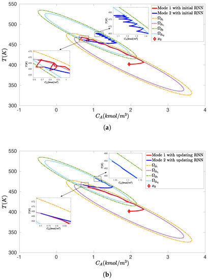
Figure 2. Closed–loop state trajectories $(C_A,T)$ for the uncertain CSTR system operating in mode 1 for $t\in [0,0.25$ h) (red solid line) and switching to mode 2 at $t=0.25$ h (blue solid line) under the RNN-LEMPC of Equation (26), (a) using the initial offline-learning RNNs at all times, and (b) using the online updating RNNs, for the initial condition $(C_A,T)$ = (1.95 kmol/m${}^3$ 402 K) (marked as red diamond).

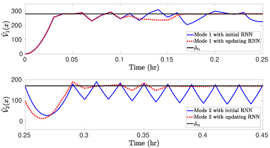
Figure 3. Comparisons of ${\widehat{V}}_1\left(x\right)$ for mode 1 and ${\widehat{V}}_2\left(x\right)$ for mode 2 under the initial offline-learning and online updating RNN models.

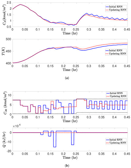
Figure 4. (a) Closed-loop state ($C_A$ and T) and (b) manipulated input ($C_{A_0}$ and Q) profiles for the uncertain CSTR system operating in mode 1 for $t\in [0,0.25$ h) and switching to mode 2 at $t=0.25$ h under the RNN-LEMPC of Equation (26) using the initial offline-learning RNNs at all times (blue solid line), and using the online updating RNNs (red dashed line), for the initial condition $(C_A,T)$ = (1.95 kmol/m${}^3$ 402 K).

Finally, in the event that the system dynamics of the CSTR remains unchanged for the remaining operation time (i.e., no further mode transition and no process disturbances after $t=0.45\mathrm{h}$), an online update of RNNs will be deactivated and the final RNN model can be derived by solving Equation (18), and the CSTR will operate in mode 2 under the LEMPC using the final RNN model after $t=0.45\mathrm{h}$. Specifically, when the CSTR operates in mode 2, the RNNs are updated online at $t=0.3,0.35,0.4,0.45$ for four times (the number of rounds $T=4$). We use the hypothesis $h_1$ and a sequence of hypotheses $h_2,\dots ,h_5$ to denote the initial RNN and the four online updating RNNs for mode 2, respectively. To simplify the calculation of the empirical discrepancy ${\widehat{disc}}_{\mathcal{H}}\left(\lambda \right)$ of Equation (18), the hypothesis $\overline{h}$ is considered to belong to a linear space (denoted by $\overline{\mathcal{H}}$ of the hypotheses $h_2,\dots ,h_5$ in this example, that is $\overline{h}\in \overline{\mathcal{H}}:=\left\{{\sum }_{i=1}^4{\beta }_i{h}_{i+1},\mathrm{where}{\sum }_{i=1}^4{\beta }_i=1\mathrm{and}{\beta }_i\ge 0\forall i=1,\dots ,4\right\}$. It is noted that each round of online learning represents five sampling periods in this example, and, thus, the RNN input for the next round $X_{T+1}$ consists of the system states $x\left(t\right)$ and the control inputs $u\left(t\right)$ for the current and the next four sampling steps, where $t=0.45,0.46,0.47,0.48,$ and $0.49\mathrm{h}$. Therefore, the loss between the RNN outputs predicted by the hypotheses $h_{t+1}$ and $\overline{h}$ on $X_{T+1}$ (i.e., $L\left(h_{t+1}\left(X_{T+1}\right),\overline{h}\left(X_{T+1}\right)\right)$, $t=1,\dots ,4$) can be obtained. The optimization problem of Equation (18) can be simplified to the following minimax optimization problem:

$$\begin{array}{cc}\hfill \underset{\lambda \in {\Omega }_T}{min}\underset{\overline{h}\in \overline{\mathcal{H}}}{max}& \left|\sum _{t=1}^T{\lambda }_t\left(L\left(h_{t+1},Z_{t+1}\right)-L\left(h_{t+1}\left(X_{T+1}\right),\overline{h}\left(X_{T+1}\right)\right)\right)\right|+\sum _{t=1}^T{\lambda }_{t}L\left(h_{t+1},Z_{t+1}\right)\hfill \\ \hfill & s.t.{\lambda }_T=0,\sum _{t=1}^T|{\lambda }_t-\frac{1}{T}|\le \alpha \hfill \end{array}$$

(34)

It is noted that exhaustive searches for the hypothesis $\overline{h}$ are performed in the linear space $\overline{\mathcal{H}}$, thereby converting the minimax optimization problem of Equation (34) into the minimization problem of the maximum of a set of objective functions, which can be efficiently solved using the MATLAB routine fminimax. By setting the hyperparameter $\alpha =0.8$, the optimization problem of Equation (34) is solved to calculate the optimal weight vector $\lambda =({\lambda }_1\dots {\lambda }_4)$, yielding ${\lambda }_1=0.1$, ${\lambda }_2=0.25$, ${\lambda }_3=0.65$, where the weight ${\lambda }_4$ is assigned to be zero following the constraints in Equation (34). Subsequently, the final RNN model h is derived using the ensemble of the hypotheses $h_2,\dots ,h_4$ with the corresponding weights ${\lambda }_1\dots {\lambda }_3$, that is $h={\sum }_{t=1}^3{\lambda }_t{h}_{t+1}$, and the hypothesis $h_5$ is discarded due to its weight ${\lambda }_4=0$. It should be pointed out that when the system dynamics of the CSTR varies over time caused by further mode transitions and/or process disturbances at some future operation time, the final model h needs to be updated online again using real-time data if it does not perform well.

5.2. The CSTR Switched between Two Steady-States without Disturbances

We next consider a special switching case of the nominal CSTR system, as discussed in Section 3.1, where the CSTR operates in mode 1 defined in Section 5.1 at all times (i.e., $\sigma \equiv 1$ for Equation (32)) and does not involve disturbances. In this case, two steady-states $(C_{A{s}_1},T_{s_1})$ = (1.95 kmol/m${}^3$, 402 K) and $(C_{A{s}_2},T_{s_2})$ = (1.22 kmol/m${}^3$, 438 K) for the CSTR are considered under $\left(C_{A{0}_s}{Q}_s\right)$ = (4 kmol/m${}^3$, 0 kJ/h). The CSTR is switched between two steady-states at the prescribed switching times while maximizing the economic costs of Equation (33) under RNN-LEMPC. The CSTR is said to operate in mode 1 or 2 when it operates in the stability region ${\Omega }_{{\widehat{\rho }}_1}$ or ${\Omega }_{{\widehat{\rho }}_2}$ around the steady-state $(C_{A{s}_1},T_{s_1})$ or $(C_{A{s}_2},T_{s_2})$. For both modes, the control Lyapunov functions follow those in Section 5.1 with $P_1=P_2=\left[\begin{array}{cc}1060& 22\\ 22& 0.52\end{array}\right]$. In this section, it is assumed that historical operational data is only available for the CSTR operating in a portion of operating region (denoted by ${\Omega }_0$) around the steady-state $(C_{A{s}_1},T_{s_1})$, where ${\Omega }_0:=\left\{1.5{\mathrm{kmol}/\mathrm{m}}^3\le C_A\le 2.4{\mathrm{kmol}/\mathrm{m}}^3\mathrm{and}360K\le T\le 440K\right\}$ (marked as a rectangle in Figure 5). Based on this limited training dataset, an initial RNN is trained using the same method in Section 5.1. The stability region ${\Omega }_{{\widehat{\rho }}_1}$ and a subset ${\Omega }_{{\widehat{\rho }}_{e_1}}$ for mode 1 follow those in Section 5.1 with ${\widehat{\rho }}_1=368$ and ${\widehat{\rho }}_{e_1}=280$, and the stability region ${\Omega }_{{\widehat{\rho }}_2}$ with ${\widehat{\rho }}_2=480$ and a subset ${\Omega }_{{\widehat{\rho }}_{e_2}}$ with ${\widehat{\rho }}_{e_2}=380$ are chosen for the CSTR at mode 2 in this section. In this example, since the initial RNN is developed with the dataset in ${\Omega }_0$ around the steady-state $(C_{A{s}_1},T_{s_1})$ of mode 1, we will operate the CSTR in mode 1 under LEMPC with the initial RNN at all times. However, when the CSTR operates in mode 2, we will update the RNN models online since the initial RNN lacks the dataset around the steady-state $(C_{A{s}_2},T_{s_2})$ of mode 2. Specifically, starting from the initial RNN, the RNNs are updated online using the most recent real-time data (i.e., every five sampling periods for each round) and the previous RNN model.

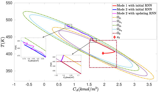
Figure 5. Closed-loop state trajectories $(C_A,T)$ for the nominal CSTR system operating in mode 1 for $t\in [0,0.1\mathrm{h})$ using the initial offline-learning RNN (red solid line), and switching to mode 2 at $t=0.1\mathrm{h}$ using the initial RNN (blue solid line) and online updating RNNs (pink dashed line) under the RNN-LEMPC of Equation (26) with the initial condition $(C_A,T)=\left(1.95{\mathrm{kmol}/\mathrm{m}}^{3}402\mathrm{K}\right)$ (marked as red diamond).

The simulation results for the nominal CSTR system switched between two steady-states under the RNN-LEMPC of Equation (26) are presented in Figure 5 and Figure 6. Specifically, the CSTR starts from an initial condition $(C_A,T)=\left(1.95{\mathrm{kmol}/\mathrm{m}}^{3}402\mathrm{K}\right)$ and operates in mode 1 for $t\in [0,0.1\mathrm{h})$ under the LEMPC with the initial RNN constructed with the dataset in ${\Omega }_0$. Subsequently, the CSTR operates under mode 2 for $t\in [0.1\mathrm{h},\infty )$ (i.e., the remaining operation time) following a switching schedule from mode 1 to mode 2 at $t=0.1\mathrm{h}$ under LEMPC using the initial RNN and the online updating RNNs. Figure 5 shows that under the initial RNN, the state trajectory closely follows the boundary of ${\Omega }_{{\widehat{\rho }}_{e_1}}$ for mode 1. This is consistent with the result in Figure 6a, which shows that the Lyapunov function value ${\widehat{V}}_1\left(x\right)$ under the initial RNN converges to ${\widehat{\rho }}_{e_1}$ after $t=0.04\mathrm{h}$. It should be mentioned that the initial RNN is constructed with the dataset gathered from a portion of the operating region around $(C_{A{s}_1},T_{s_1})$, and, thus, the LEMPC with the initial RNN performs well for the CSTR operating in mode 1. Additionally, it is observed in Figure 5 that under the initial RNN, there exists a gap between the closed-loop state trajectory and the boundary of ${\Omega }_{{\widehat{\rho }}_{e_2}}$ for mode 2, while the closed-loop state trajectory under the online updating RNNs ultimately operates near the boundary of ${\Omega }_{{\widehat{\rho }}_{e_2}}$ after exhibiting oscillations for some sampling steps. It is more apparent in Figure 6b that the Lyapunov function value ${\widehat{V}}_2\left(x\right)$ under the initial RNN converges to a value of 340, while it converges to ${\widehat{\rho }}_{e_2}=380$ after $t=0.26\mathrm{h}$ under the online updating RNNs. The total economic benefits $L_E={\int }_{0.15}^{0.4}{l}_e(x,u)dt$ within the operating period $t\in [0.15\mathrm{h},0.4\mathrm{h})$ are calculated (note that the first update of RNNs occurs at $t=0.15\mathrm{h}$), which yields 4.75 and 4.84 for the LEMPC with the initial RNN and the online RNNs, respectively. Therefore, the accumulative economic benefits during $t\in [0.15\mathrm{h},0.4\mathrm{h})$ are improved by $1.9\%$ via online learning. Finally, the RNNs are updated online at $t=0.15,0.2,0.25,0.3,0.35,0.4\mathrm{h}$ six times ($T=6$) to generate a sequence of hypotheses $h_2,\dots ,h_7$. Based on the testing error $L(h_t,Z_t)$ for each hypothesis $h_t$, Equation (8) is solved with the hyperparameter $\alpha =0.6$ to calculate the optimal weights ${\lambda }_1\dots {\lambda }_6$ for the hypotheses $h_1,\dots ,h_6$, respectively, yielding ${\lambda }_1=0$, ${\lambda }_2=0.0333$, ${\lambda }_3=0.1666$, ${\lambda }_4=0.1667$, ${\lambda }_5=0.4667$, and ${\lambda }_6=0.1667$. Subsequently, the final RNN model h is developed with $h={\sum }_{t=1}^6{\lambda }_t{h}_t$, and the CSTR operates in mode 2 under the LEMPC with this final RNN model for the remaining operation time. However, when there is a further mode transition for the CSTR, the online update of RNNs is required to perform again if the final model does not predict well for the CSTR operating in the new mode.

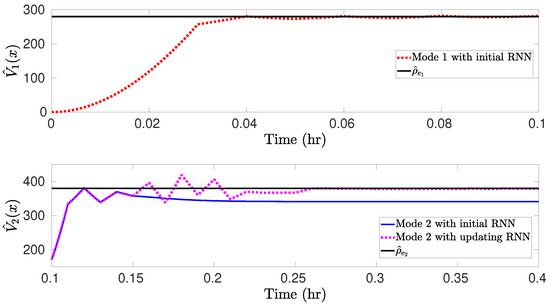
Figure 6. Comparisons of ${\widehat{V}}_1\left(x\right)$ for mode 1 using the initial offline-learning RNN (red dashed line), and ${\widehat{V}}_2\left(x\right)$ for mode 2 using the initial RNN (blue solid line) and online updating RNNs (pink dashed line).

6. Conclusions

This work proposed an LEMPC scheme using online updating RNNs that can optimize the economic benefits of switched non-linear systems. The generalized error bounds for RNN models updated online in i.i.d. and non-i.i.d. settings were derived, respectively. Subsequently, the LEMPC that incorporates online learning RNNs was developed to maintain the closed-loop state within the prescribed stability region and maximize the economic benefits for the uncertain system involving bounded disturbances. A Lyapunov-based constraint was incorporated into the LEMPC formulation to ensure the success of scheduled mode transitions. Closed-loop stability for the uncertain non-linear system subject to bounded disturbances under LEMPC was proved in a probabilistic manner accounting for the generalized error bound. The proposed LEMPC scheme was applied to a chemical process example to demonstrate that economic optimality and closed-loop stability can be improved under the LEMPC using online RNNs compared to those using the initial RNNs at all times.

References

- Angeli, D.; Amrit, R.; Rawlings, J.B. On average performance and stability of economic model predictive control. IEEE Trans. Autom. Control 2011, 57, 1615–1626. [Google Scholar] [CrossRef]
- Heidarinejad, M.; Liu, J.; Christofides, P.D. Economic model predictive control of nonlinear process systems using Lyapunov techniques. AIChE J. 2012, 58, 855–870. [Google Scholar] [CrossRef]
- Müller, M.A.; Angeli, D.; Allgöwer, F. Economic model predictive control with self-tuning terminal cost. Eur. J. Control 2013, 19, 408–416. [Google Scholar] [CrossRef]
- Ellis, M.; Durand, H.; Christofides, P.D. A tutorial review of economic model predictive control methods. J. Process Control 2014, 24, 1156–1178. [Google Scholar] [CrossRef]
- Dong, Z.; Angeli, D. Analysis of economic model predictive control with terminal penalty functions on generalized optimal regimes of operation. Int. J. Robust Nonlinear Control 2018, 28, 4790–4815. [Google Scholar] [CrossRef]
- Dong, Z.; Angeli, D. Homothetic tube-based robust economic mpc with integrated moving horizon estimation. IEEE Trans. Autom. Control 2020, 66, 64–75. [Google Scholar] [CrossRef]
- Lee, T.C.; Jiang, Z.P. Uniform asymptotic stability of nonlinear switched systems with an application to mobile robots. IEEE Trans. Autom. Control 2008, 53, 1235–1252. [Google Scholar] [CrossRef]
- Shen, H.; Xing, M.; Wu, Z.G.; Xu, S.; Cao, J. Multiobjective fault-tolerant control for fuzzy switched systems with persistent dwell time and its application in electric circuits. IEEE Trans. Fuzzy Syst. 2019, 28, 2335–2347. [Google Scholar] [CrossRef]
- Jin, Y.; Fu, J.; Zhang, Y.; Jing, Y. Reliable control of a class of switched cascade nonlinear systems with its application to flight control. Nonlinear Anal. Hybrid Syst. 2014, 11, 11–21. [Google Scholar] [CrossRef]
- Branicky, M.S. Multiple Lyapunov functions and other analysis tools for switched and hybrid systems. IEEE Trans. Autom. Control 1998, 43, 475–482. [Google Scholar] [CrossRef]
- Aleksandrov, A.Y.; Chen, Y.; Platonov, A.V.; Zhang, L. Stability analysis for a class of switched nonlinear systems. Automatica 2011, 47, 2286–2291. [Google Scholar] [CrossRef]
- Hespanha, J.P.; Morse, A.S. Stability of switched systems with average dwell-time. In Proceedings of the 38th IEEE Conference on Decision and Control, Phoenix, AZ, USA, 7–10 December 1999; Volume 3, pp. 2655–2660. [Google Scholar]
- Xiang, W.; Xiao, J. Stabilization of switched continuous-time systems with all modes unstable via dwell time switching. Automatica 2014, 50, 940–945. [Google Scholar] [CrossRef]
- Nodozi, I.; Rahmani, M. LMI-based model predictive control for switched nonlinear systems. J. Process Control 2017, 59, 49–58. [Google Scholar] [CrossRef]
- Mhaskar, P.; El-Farra, N.H.; Christofides, P.D. Predictive control of switched nonlinear systems with scheduled mode transitions. IEEE Trans. Autom. Control 2005, 50, 1670–1680. [Google Scholar] [CrossRef]
- Heidarinejad, M.; Liu, J.; Christofides, P.D. Economic model predictive control of switched nonlinear systems. Syst. Control Lett. 2013, 62, 77–84. [Google Scholar] [CrossRef]
- Prabhu, S.; Deepa, S.; Arulperumjothi, M.; Susilowati, L.; Liu, J. Resolving-power domination number of probabilistic neural networks. J. Intell. Fuzzy Syst. 2022, 43, 6253–6263. [Google Scholar] [CrossRef]
- Zheng, Y.; Zhang, T.; Li, S.; Qi, C.; Zhang, Y.; Wang, Y. Data-Driven Distributed Model Predictive Control of Continuous Nonlinear Systems with Gaussian Process. Ind. Eng. Chem. Res. 2022, 61, 18187–18202. [Google Scholar] [CrossRef]
- Zhang, T.; Li, S.; Zheng, Y. Implementable Stability Guaranteed Lyapunov-Based Data-Driven Model Predictive Control with Evolving Gaussian Process. Ind. Eng. Chem. Res. 2022, 61, 14681–14690. [Google Scholar] [CrossRef]
- Pan, Y.; Wang, J. Model predictive control of unknown nonlinear dynamical systems based on recurrent neural networks. IEEE Trans. Ind. Electron. 2011, 59, 3089–3101. [Google Scholar] [CrossRef]
- Xu, J.; Li, C.; He, X.; Huang, T. Recurrent neural network for solving model predictive control problem in application of four-tank benchmark. Neurocomputing 2016, 190, 172–178. [Google Scholar] [CrossRef]
- Shahnazari, H.; Mhaskar, P.; House, J.M.; Salsbury, T.I. Modeling and fault diagnosis design for HVAC systems using recurrent neural networks. Comput. Chem. Eng. 2019, 126, 189–203. [Google Scholar] [CrossRef]
- Wu, Z.; Christofides, P.D. Economic machine-learning-based predictive control of nonlinear systems. Mathematics 2019, 7, 494. [Google Scholar] [CrossRef]
- Wu, Z.; Rincon, D.; Christofides, P.D. Real-time adaptive machine-learning-based predictive control of nonlinear processes. Ind. Eng. Chem. Res. 2019, 59, 2275–2290. [Google Scholar] [CrossRef]
- Wagener, N.; Cheng, C.A.; Sacks, J.; Boots, B. An online learning approach to model predictive control. arXiv 2019, arXiv:1902.08967. [Google Scholar]
- Bieker, K.; Peitz, S.; Brunton, S.L.; Kutz, J.N.; Dellnitz, M. Deep model predictive control with online learning for complex physical systems. arXiv 2019, arXiv:1905.10094. [Google Scholar]
- Ning, C.; You, F. Online learning based risk-averse stochastic MPC of constrained linear uncertain systems. Automatica 2021, 125, 109402. [Google Scholar] [CrossRef]
- Zheng, Y.; Zhao, T.; Wang, X.; Wu, Z. Online Learning-Based Predictive Control of Crystallization Processes under Batch-to-Batch Parametric Drift. AIChE J. 2022, 68, e17815. [Google Scholar] [CrossRef]
- Cesa-Bianchi, N.; Conconi, A.; Gentile, C. On the generalization ability of on-line learning algorithms. IEEE Trans. Inf. Theory 2004, 50, 2050–2057. [Google Scholar] [CrossRef]
- Cesa-Bianchi, N.; Gentile, C. Improved risk tail bounds for on-line algorithms. IEEE Trans. Inf. Theory 2008, 54, 386–390. [Google Scholar] [CrossRef]
- Kakade, S.M.; Tewari, A. On the generalization ability of online strongly convex programming algorithms. Adv. Neural Inf. Process. Syst. 2008, 21, 801–808. [Google Scholar]
- Rakhlin, A.; Sridharan, K.; Tewari, A. Online learning via sequential complexities. J. Mach. Learn. Res. 2015, 16, 155–186. [Google Scholar]
- Kuznetsov, V.; Mohri, M. Time series prediction and online learning. In Proceedings of the 29th Annual Conference on Learning Theory, New York, NY, USA, 23–26 June 2016; pp. 1190–1213. [Google Scholar]
- Hu, C.; Cao, Y.; Wu, Z. Online Machine Learning Modeling and Predictive Control of Nonlinear Systems with Scheduled Mode Transitions. AIChE J. 2022, 69, e17882. [Google Scholar] [CrossRef]
- Hu, C.; Wu, Z. Model Predictive Control of Switched Nonlinear Systems Using Online Machine Learning. submitted.
- Lin, Y.; Sontag, E.D. A universal formula for stabilization with bounded controls. Syst. Control Lett. 1991, 16, 393–397. [Google Scholar] [CrossRef]
- Wu, Z.; Tran, A.; Rincon, D.; Christofides, P.D. Machine learning-based predictive control of nonlinear processes. Part I: Theory. AIChE J. 2019, 65, e16729. [Google Scholar] [CrossRef]
- Wu, Z.; Rincon, D.; Gu, Q.; Christofides, P.D. Statistical Machine Learning in Model Predictive Control of Nonlinear Processes. Mathematics 2021, 9, 1912. [Google Scholar] [CrossRef]
- Kuznetsov, V.; Mohri, M. Discrepancy-based theory and algorithms for forecasting non-stationary time series. Ann. Math. Artif. Intell. 2020, 88, 367–399. [Google Scholar] [CrossRef]
- Wu, Z.; Alnajdi, A.; Gu, Q.; Christofides, P.D. Statistical machine-learning–based predictive control of uncertain nonlinear processes. AIChE J. 2022, 68, e17642. [Google Scholar] [CrossRef]
- Wächter, A.; Biegler, L.T. On the implementation of an interior-point filter line-search algorithm for large-scale nonlinear programming. Math. Program. 2006, 106, 25–57. [Google Scholar] [CrossRef]
Disclaimer/Publisher’s Note: The statements, opinions and data contained in all publications are solely those of the individual author(s) and contributor(s) and not of MDPI and/or the editor(s). MDPI and/or the editor(s) disclaim responsibility for any injury to people or property resulting from any ideas, methods, instructions or products referred to in the content. |
© 2023 by the authors. Licensee MDPI, Basel, Switzerland. This article is an open access article distributed under the terms and conditions of the Creative Commons Attribution (CC BY) license (https://creativecommons.org/licenses/by/4.0/).