1. Introduction
The iron and steel industry will undergo a very important transformation in the coming decades to decarbonize the ironmaking process. Currently, the iron and steel industry is responsible for approximately 2.6 Gt CO
2 emissions annually, which is about 7% of total CO
2 emissions or 25% of total industrial CO
2 emissions [
1,
2]. The main cause of CO
2 emissions in the ironmaking process is the use of carbon-based reducing agents such as coal and coke for the removal of oxygen from iron ores and high energy demand as a result of high operating temperatures [
3]. The total steel production in the year 2022 was reported to be 1878.5 Mt, more than 80% of which was produced using the conventional blast furnace—basic oxygen furnace (BF-BOF) route, which relies on coke for its operation with an energy demand of 18 GJ/t
steel while emitting 1870–2030 kg CO
2/t
lsteel [
4,
5,
6]. To address the problem of CO
2 emissions in the ironmaking process, the directly reduced iron (DRI) process was commercialized, which uses reformed natural gas instead of coke to reduce iron ore pellets to metallic iron in solid state, followed by steelmaking using an electric arc furnace (EAF) [
7]. However, the DRI-EAF route is not able to completely eliminate CO
2 emissions from the ironmaking process as it operates on reformed natural gas, which is a carbon-containing reducing agent. The DRI-EAF route is able to reduce CO
2 emissions to 970–1110 kg CO
2/t
lsteel, which is approximately 50% less CO
2 emissions compared with the conventional BF-BOF route [
6,
8].
To eliminate CO
2 emissions almost completely from the ironmaking process, it is necessary to use an alternate reducing agent that is not carbon-based. Recently, H
2 has gained increased attention from policymakers and major stakeholders in the industry to replace carbon-based reducing agents for the ironmaking process. Numerous studies in the last 80 years have been conducted to understand the effect of H
2 on the reduction kinetics and properties of pellets, such as porosity, swelling, and compressive strength on a laboratory scale [
9,
10,
11,
12,
13,
14,
15,
16]. However, very few studies have reported the implementation of H
2 as a reducing agent for the ironmaking process on a pilot scale with a moving bed [
17]. The use of H
2 for ironmaking on a small industrial scale was first reported by the Circored plant in Trinidad and Tobago, which operated between 1999 and 2001 and 2004–2006. However, Circored used fluidized bed technology instead of pellets or lump ore reduction, and its operation was not commercially viable [
18]. Another large-scale hydrogen-based ironmaking development that is currently underway is the Hydrogen Breakthrough Ironmaking Technology (HYBRIT) project, which was started in 2016 by three companies in Sweden, namely LKAB (Luossavaara-Kiirunavaara Aktiebolag, mining company), SSAB (steel company), and Vattenfall AB (energy company) [
19]. It is scheduled to produce H
2-based steel at a production scale (1.3 Mt/year) by 2026 [
20]. The HYBRIT project aims to use renewable electricity to produce H
2 and use it for fossil-free steel manufacturing with a very low CO
2 footprint [
21]. On a larger scale, H2 Green Steel, also based in Sweden, aims to produce fossil-free steel at a production rate of 2.5 Mt/year starting in the year 2025 at their plant in Boden, utilizing hydroelectric power availability [
22]. Recently, Salzgitter AG, Germany, was also awarded 1 Billion Euros to make an industrial scale ironmaking plant with a production capacity of 1.9 Mt [
23]. However, renewable energy is not abundant in every geographic location where iron and steel are manufactured, and moreover, its availability may be dependent on the intermittency of solar and wind and therefore, the cost of production of green H
2 still remains very high—in the range of 4–7 USD/kg [
24,
25]. The total landed cost of green hydrogen was reported as 4.5 USD/kg in a previous study focusing on techno-economic analysis using available data from the year 2019 before the COVID-19 pandemic [
6].
The Grid-Interactive Steelmaking with Hydrogen (GISH) project, a collaboration between Missouri S&T, Arizona State University, Nucor Corporation, Danieli Corporation, ArcelorMittal, Steel Dynamics, Inc., Gerdau, Linde Inc., Air Liquide America Corporation, and National Renewable Energy Laboratory (NREL), is aimed at demonstrating a pilot-scale reactor which can operate flexibly using H2 and a mixture of H2 with natural gas to produce 1 Mt/week of DRI. This pilot reactor will serve as a base design for larger industrial-scale reactors to be built in the future that can operate using both natural gas and H2 as a reducing agent, depending on the availability of affordable renewable energy for hydrogen electrolysis. This reactor flexibility will mitigate the risk of investment by industries as it will ensure that production is not disrupted in times when H2 is not available for reduction. Another mission of the project is to produce enough H2-reduced metalized pellets to facilitate industrial-scale melting trials. This study reports the steady-state temperature profiles inside the GISH pilot reactor along with the metallization of DRI produced using pure H2 as a reducing agent.
To start and commission a DRI reactor, it is very important to approximately optimize the operational parameters such as feed flow, the temperature of the external heating coil, and the inlet gas flow rate along with its temperature. Modeling and simulation are powerful tools to predict the output of a DRI reactor for a set of input parameters. Previous studies have reported the modeling and simulation of pilot-scale reactors and industrial-scale reactors, such as the Midrex process and the Energiron process. Dalle Nogare, Daniela, et al., and Dario Pauluzzi et al. reported a CFD model for the DRI shaft furnace developed at Danieli & C Officine Meccaniche [
26,
27]. Da Costa, A., et al. reported a model of a shaft furnace operating with pure H
2 as a reducing agent made using FORTRAN and finite volume method [
28]. Hamadeh, H., et al. modified the model as reported by Da Costa, A., et al. making it more sophisticated, which can be applied to both MIDREX and Energiron processes [
29]. AZ Ghadi, et al. also reported a model based on the finite volume technique for a MIDREX shaft reactor [
30]. This study reports the modeling and simulation of the GISH pilot reactor operated on H
2 using finite element analysis using COMSOL Multiphysics version 5.6 software. The measured output metallization and reactor temperature profiles for controlled, steady-state operating conditions are used to assess the model performance.
2. Materials, Methods, and Pilot Plant Operation Conditions
Five tons of hematite pellets used for the pilot plant trials were supplied by Voestalpine AG, Linz, Austria, from the plant in Corpus Christi, TX, USA (now ArcelorMittal). The hematite pellets consisted of 67.8% Fe (total), 1.34% SiO2, 0.76% CaO, 0.49% Al2O3, and 0.13% volatiles. A volume of 140,000 cubic feet (3964.35 cubic meters) of H2 was supplied by Airgas, Radnor, PA. The GISH project pilot plant was constructed by Hazen Research Inc., Golden, CO, with design input from Danieli and our other industry partners.
The GISH project pilot plant is located at the Hazen Research Inc. campus in Golden, CO.
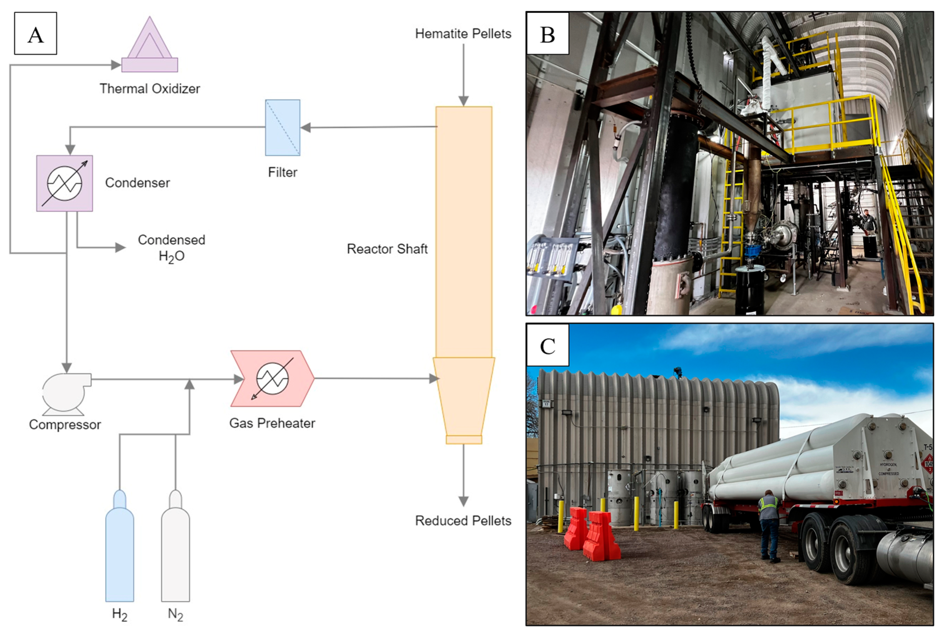
Figure 1A shows a simplified process schematic of the GISH pilot plant. Data for two different operation scenarios are reported in this study at a steady state, as shown in
Table 1. To operate the pilot plant, H
2 gas from the tank trailers is first fed into the gas preheater, which heats it from room temperature to the target temperatures at the reactor inlet, as shown in
Table 1. The heated gas is then fed into the reactor shaft via a bustle located between the bottom of the reactor and the pellet cooling bustle as shown in
Figure 2A,B. H
2 travels in the opposite direction to pellets from the bottom of the reactor pellet bed to the top while reducing the iron ore pellets. External heat is supplied to the reaction zone in the reactor shaft by three electrical heating zones to provide the external energy necessary for the endothermic H
2—iron oxide reduction reaction. The hematite pellets are fed at the top of the reactor at a rate of 21.4 kg/h, and the reduced iron pellets are obtained at the bottom, as shown in
Figure 2A,B. The off-gas containing H
2O and H
2 at the top of the reactor is sent to a filtration unit, which removes dust and fines from the gas mixture. The filtered gas is then passed through a condenser to remove the moisture. The remaining H
2 is then recycled into the feed using a compressor. Excess H
2 from the condenser is burnt off using a thermal oxidizer.
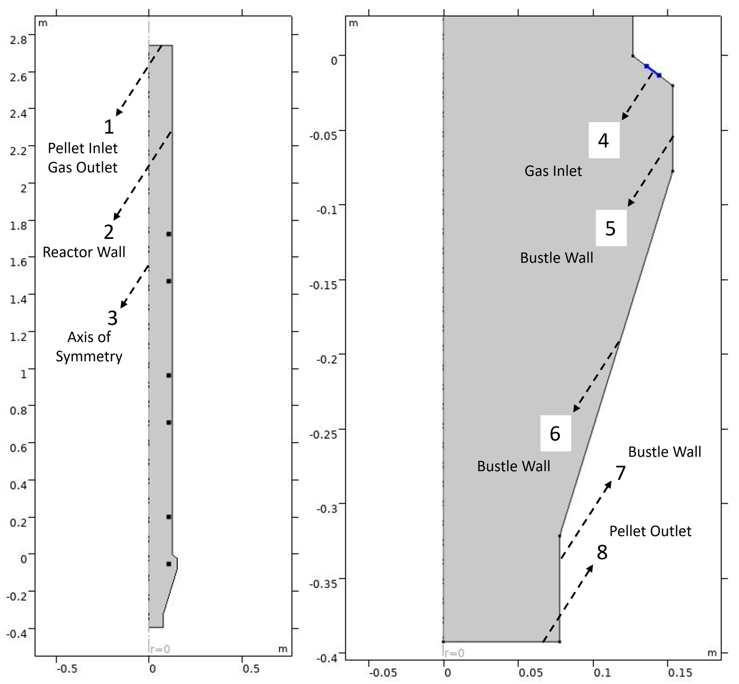
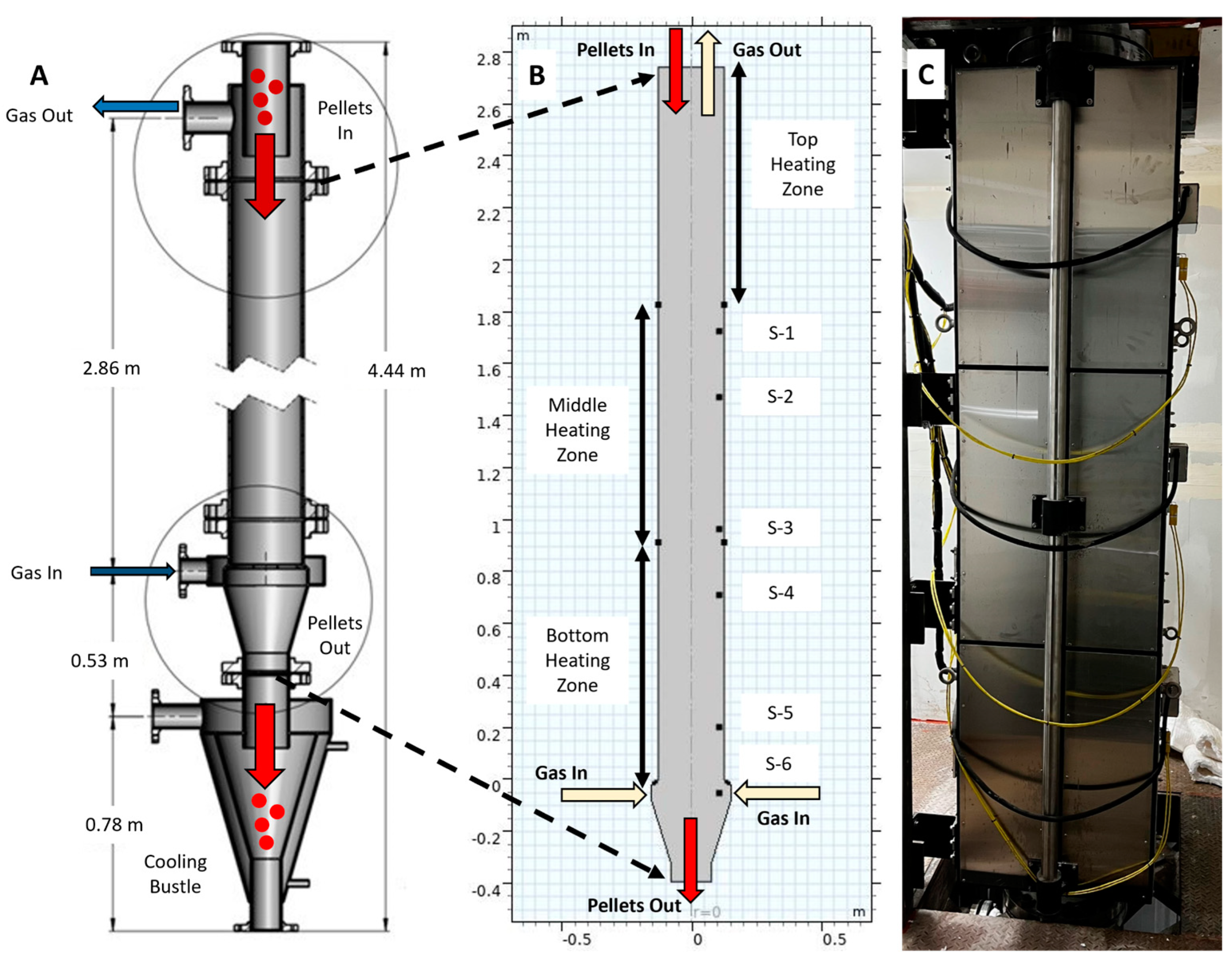
The reactor with a 0.254 m inner diameter and 2.9 m inner height consisted of three heating zones as shown in the model geometry in
Figure 2A,B. The temperature of the bottom, middle, and top heating zones was set to the temperature shown in
Table 1. If the temperature at coil sensors was higher than the set temperature, no external heating was provided. The temperature of the pellet bed was measured using six sensors placed at 1.02 m (S-1), 1.27 m (S-2), 1.78 m (S-3), 2.03 m (S-4), 2.54 m (S-5), and 2.79 m (S-6) from the top, as shown in
Figure 2B.
Pellet samples were discharged into the sealed metal bins from the outlet of the pilot reactor after they reached room temperature inside the cooling bustle with nitrogen as a cooling media. Reduced pellets were sent to ArcelorMittal, Corpus Christi, TX, to determine the metallization using the ISO 16878:2016 and ISO 2597-2:2019 methods [
31,
32]. A 1 kg sample was crushed and mixed using a pulverizing machine. A mass of 100 mg of powder was used to determine the average metallization of the sample. The metallization was calculated using Equation (1), as shown below [
33].
3. Measured Steady State Reactor Temperature Profiles and Metallization
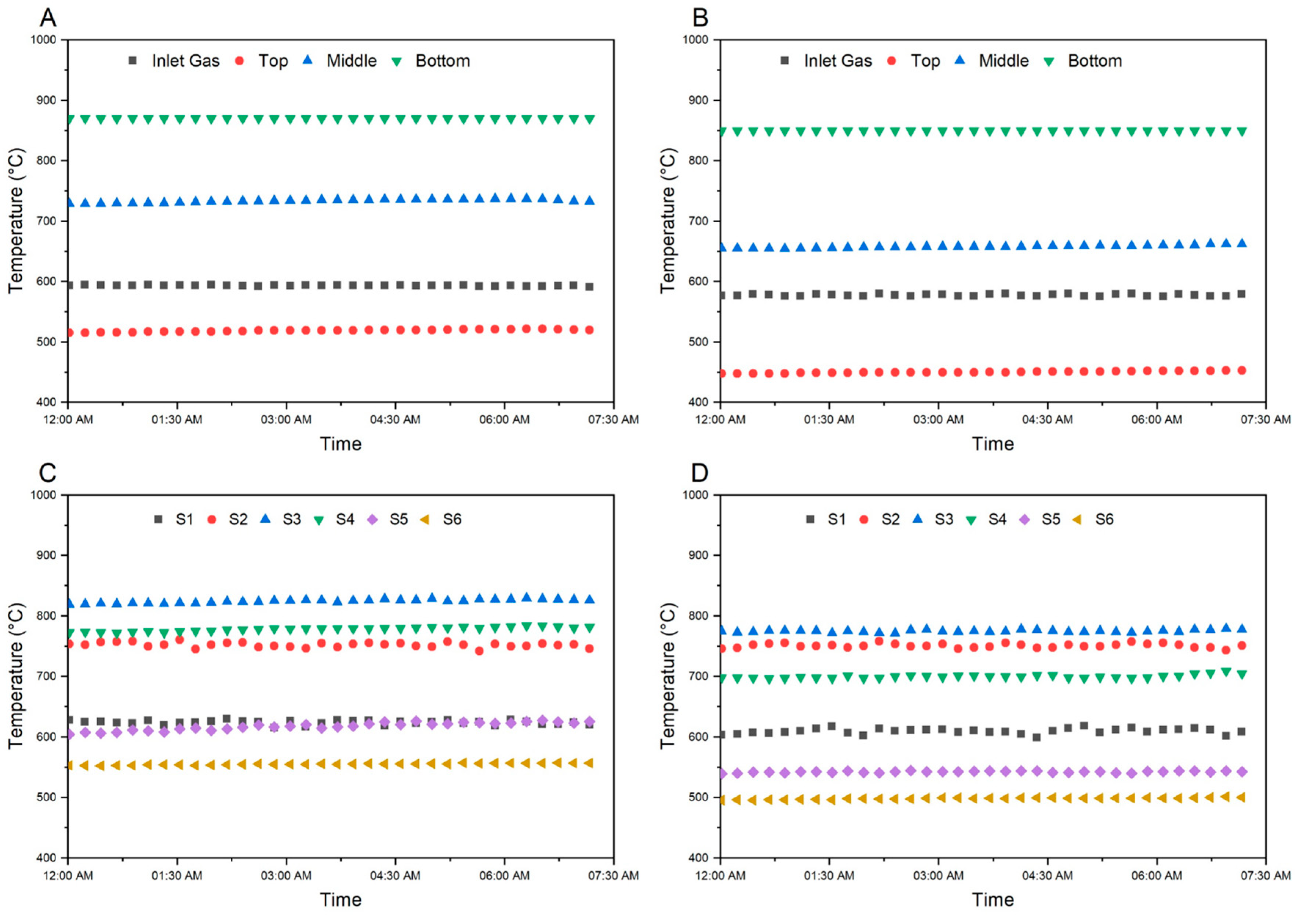
The pilot plant trials for the GISH project were performed at the Hazen Research Inc. campus in Golden, CO. The steady-state pilot plant operation data of approximately 7.5 h were reported in this study, with steady-state operations defined by the steady readings of the temperature sensors inside the reactor at a constant pellet and gas feed. The temperature readings taken from the temperature sensors between steady-state operations are reported in
Figure 3.
Figure 3A shows the steady state temperature vs. time plot of the inlet gas and the heating coil temperature sensors outside the reactor. The average temperature over the reported time period was observed to be 593.5 °C for the inlet gas, 870 °C for the bottom heating coil, 733.6 °C for the middle heating coil, and 519.0 °C for the top heating coil. Since the temperature exceeded the 300 °C set-point for both the middle and top heating coils, neither of them were provided any external heat, and they were switched off.
Figure 3C shows the steady state temperature vs. time plot of the temperature sensors placed inside the reactor to monitor the temperature of the pellet bed. The average temperature of the sensors inside the reactor was observed to be 623.5 °C for S-6, 751.9 °C for S-5, 824.6 °C for S-4, 778.1 °C for S-3, 617.9 °C for S-2 and 555.1 °C for S-1 over the reported time period. The metallization of the pellets obtained at steady state, determined using the ISO 16878:2016 and ISO 2597-2:2019 method was 91.8% for an average of four samples taken two hours apart from each other.
Similarly,
Figure 3B shows the steady state temperature vs. time plot of the inlet gas and the heating coil temperature sensors outside the reactor for Scenario 2. Data for Scenario 2 was collected two days prior to Scenario 1. The average temperature of the inlet gas was 577.6 °C, the bottom heating coil was 850.0 °C, the middle heating coil was 658.0 °C and the top heating coil was 450.4 °C, respectively. The average temperature of the sensors inside the reactor was observed to be 609.6 °C for S-6, 751.0 °C for S-5, 774.8 °C for S-4, 699.7 °C for S-3, 542.3 °C for S-2 and 498.3 °C for S-1 as shown in
Figure 3D. The metallization was observed to be 67.8% for Scenario 2 for one sample at a steady state. The metallization was higher for Scenario 1 because of the availability of a higher amount of moles of H
2 in the feed gas for reduction and higher temperature of feed gas as an increase in the moles of H
2 increases the heat carrying capacity of the bulk gas from the preheater. This was accompanied by relatively higher external heat provided for the endothermic reduction reaction with the bottom heating coil set at 870 °C in Scenario 1.
4. Numerical Modelling of the GISH Reactor Using Finite Element Analysis
4.1. Model Description and Geometry
The development of a reactor model is important for the commissioning and operation of a chemical plant as it can predict the output of a reactor for a given input. This information helps the plant operators and engineers to approximately predict the sensitivity of operational parameters, such as gas inlet temperature and composition pellet feed rate to changes in the output, i.e., metallization, temperature profiles, etc. The output of the GISH project pilot plant can be estimated by simulating the model of the H
2 direct reduction reactor shaft. The model for this study was developed using COMSOL Multiphysics 5.6, where a 2D-axisymmetric geometry was used to describe the reactor. As shown in
Figure 2A,B, the model consists of the reactor shaft and a gas inlet bustle. The hematite pellet feed enters the reactor from the top of the shaft and exits from the bottom of the gas inlet bustle, while the feed reactant gas mixture enters from the side of the inlet bustle, and the off-gas exits from the top of the reactor shaft. External heating is provided using the bottom heating zone for the endothermic reduction reaction of iron ore pellets using H
2.
For the 2-D axisymmetric model, vertices of the geometry were defined in terms of height and radial distance from the center. The model geometry was built using the rectangular shape of width 0.254 m and height 2.743 m for the reactor shaft (real dimensions), and the gas inlet bustle was built using line segments. The entire geometry was merged to form a union using the Boolean function in the geometry interface. The walls of the reactor were divided into three equal parts to represent the external heating coils, as shown in
Figure 2. Six points were defined inside the reactor to represent the temperature sensors placed inside the reactor: S-1 (1.02 m from top), S-2 (1.27 m from top), S-3 (1.78 m from top), S-4 (2.03 m from top), S-5 (2.54 m from top) and S-6 (2.79 m from top). The changes in distance from the top due to the thermal expansion of the rod with sensors are assumed to be negligible.
Figure 4 shows the domain and boundaries of the 2D-axisymmetric model.
4.2. Assumptions Made for Building the Model
A 2D-axisymmetric geometry was assumed to build the model using the finite element analysis. The conversion of hematite to iron was assumed to be a two-step reaction, with hematite reducing to wüstite and wüstite reducing to iron since at temperatures above 570 °C, hematite to magnetite conversion is expected to be very fast [
34]. The flow of pellets was assumed to be a fluid flow flowing in a laminar regime. Gangue was assumed to be inert and negligible, with no effects on the chemical kinetics, heat, and mass balance of the reduction process.
4.3. Interfaces Used to Define Flow Profile, Heat, and Mass Balance of Solids
The flow of solid pellets inside the reactor was assumed to be a fluid flowing in a laminar flow regime as the velocity of pellets was very low (order of magnitude ~10−5 m/s) along with a very low Reynolds number (order of magnitude ~10−3). The flow, heat, and mass balance of pellets were defined using the ‘Laminar flow’, ‘Heat Transfer in Fluids’, and ‘Transport of Diluted Species’ interface, respectively, available in the physics library of COMSOL Multiphysics 5.6. The variables of these three modules were interconnected to each other using the ‘Non-isothermal Flow’ module available in the Multiphysics library. A total of four solid species were defined as variables in the model: Fe2O3, FeO, Fe, and gangue. Gangue was assumed to be inert with no effects on chemical kinetics, heat balance, or mass transport of the pellets.
To obtain the flow profile of the solid pellets from the top to the bottom of the reactor, the ‘Laminar Flow’ interface uses the simplified form of the equation for conservation of momentum and the equation for conservation of mass in the laminar flow regime as shown in Equations (2) and (3) below. The inlet for the solid flow was assigned to boundary 1, while the outlet was assigned to boundary 8, as shown in
Figure 4. The inflow boundary condition of pellets was defined in terms of a normal mass flow rate of 21.4 kg/h. A slip condition (
) was assumed for boundaries 2, 4, 5, and 7, while a no-slip condition (
) was assumed for boundary 6.
The evolution of chemical concentrations of the solid species was modeled using the ‘Transport of Diluted Species’ interface. This interface can simulate the evolution of the concentration of species transported by convection, migration, and diffusion. At a steady state, this interface solves the mass conservation equation for all the defined species transported through diffusion and convection undergoing a chemical reaction, as shown in its governing equation (Equation (4)). The inflow concentrations of solid species at boundary 1 were defined using the Danckwerts Flux boundary conditions as shown in Equation (5), and the outflow was assigned to boundary 8 [
35,
36]. A No-Flux condition was assigned to all the remaining boundaries of the reactor geometry, as shown in Equation (6). The derivation and detailed theory for Equations (2)–(6) can be found in the CFD Module User’s Guide of COMSOL Multiphysics [
37]. The chemical reactions for each solid species were defined in the domain of the reactor geometry with variable reaction rates.
The temperature profile of the solid species was obtained using the ‘Heat Transfer in Fluids’ interface. This interface can solve the heat balance equation for fluids at a steady state by accounting for conduction, convection, radiation, and chemical reaction, as shown in Equation (7). The pellet inflow temperature (293.15 K) was assigned to boundary 1, and the outflow temperature was applied to boundary 8. Convective cooling was applied to boundaries 6 and 7, accounting for the heat loss in the gas inlet bustle due to the air at room temperature outside. Constant temperatures were applied to boundary 2 to account for the external heat input provided for the endothermic reaction. Convective heat transfer from solid to gas, along with heat consumption due to endothermic reactions, were defined as variables in the entire domain of the reactor geometry. The derivation and detailed theory for Equation (7) can be found in the Heat Transfer Module User’s Guide of COMSOL Multiphysics [
38].
The three different interfaces were coupled together using the ‘Reacting Flow, Diluted Species’ and ‘Non-isothermal Flow’ modules available in the ‘Multiphysics’ interface. The variable temperature from ‘Heat Transfer in Fluids’ was used to obtain the flow profile in the ‘Laminar Flow’ interface using the ‘Non-isothermal Flow.’ Further, the concentration profiles in the ‘Transport of Diluted Species’ were obtained using the temperature and velocity profiles with the help of ‘Reacting Flow, Diluted Species’.
4.4. Interfaces Used to Define Flow Profile, Heat and Mass Balance of Gases
The flow of gases inside the reactor was assumed to flow in porous media as the gas flows through the porous pellet bed from the bottom to the top of the reactor. The flow, heat, and mass balance of gases were defined using the ‘Brinkman Equations,’ ‘Heat Transfer in Fluids,’ and ‘Transport of Diluted Species’ interface, respectively. The variables for these three modules were interconnected using the ‘Non-isothermal Flow’ and ‘Reacting Flow, Diluted Species’ modules available in the Multiphysics library. A total of three gas species were defined as variables in the model: H2, H2O, and N2.
The flow profile of fluids in the porous media can be obtained using the ‘Brinkman Equations’ interface. These equations are formed by combining the continuity equation and the momentum balance equation, as shown in Equations (8) and (9) at a steady state (neglecting the Stokes flow inertial term). For the given boundary conditions, this module gives the profiles for Darcy velocity and the pressure distribution inside the domain of the defined geometry. The inlet for the gas flow was assigned to boundary 4, while the outlet was assigned to boundary 1, as shown in
Figure 4. The inflow boundary condition of gases was defined in terms of normal mass flow rate derived from a volumetric flow of H
2 feed mixed with recycled H
2 from the reactor outlet. The total content of H
2 was assumed to be 97.4% and 99.4% for Scenarios 1 and 2, respectively, while the content of H
2O was assumed to be 2.6% and 0.6% for Scenarios 1 and 2, respectively. No slip conditions were assigned to all the boundaries representing the walls of the reactor (
).
To obtain the concentration profile of gaseous species flowing through the pellet bed, the ‘Transport of Diluted Species in Porous Media’ interface was used. Equation (10) gives the governing equation for this interface. The inflow concentrations of gaseous species at boundary 4 were defined using the Danckwerts Flux boundary conditions as shown in Equation (11), and the outflow was assigned to boundary 1. A constant concentration of N2 was applied to boundary 8, accounting for the small amount of N2 leaking inside the reactor from the pellet discharge system and the cooling bustle. The No Flux condition was assigned to all the remaining boundaries of the reactor geometry, as shown in Equation (12). As with the solid species, the chemical reactions for each gaseous species were defined in the domain of the reactor geometry with variable reaction rates.
Also, as with the solid species, the ‘Heat Transfer in Fluids’ interface was used to obtain the temperature profile of the gaseous species. Equation (13) shows the governing equation for this interface. The inflow temperature was assigned to boundary 4, and the outflow temperature was applied to boundary 1. Convective cooling was applied to boundaries 6 and 7, accounting for the heat loss in the gas inlet bustle, similar to the cooling of solid species. The cooling due to N2 leaking into the reactor was accounted for by applying a temperature of 100 °C to boundary 8. Convective heat transfer from solid to gas was defined as a variable in the entire domain of the reactor geometry.
The three different interfaces were coupled together using the ‘Reacting Flow, Diluted Species’ and ‘Non-isothermal Flow’ modules available in the ‘Multiphysics’ interface similar to that used for the solid species.
4.5. Variables Used for the Chemical Kinetics and Properties of Solid and Gas Species
4.5.1. Rate of Chemical Reactions between Gas and Solid Species
The rates of chemical reactions were defined as per the 2-interface model reported by Hara et al. [
39]. This model gives analytical equations that can be used as variables in the reactor model to define the chemical reactions involved in the iron ore pellet reduction process. These equations take into account the resistances of competing reaction rates due to mass transfer in gas film, diffusion in the product phase (ash layer), and chemical reaction. Equations (14) and (15) show the reaction rate variables
(hematite to wüstite) and
(wüstite to iron) which were used to define the iron ore reduction process in the GISH pilot plant reactor model.
Here,
initial radius of the pellet,
radius of unreacted Fe
2O
3 core and
radius of unreacted Fe
2O
3 core and FeO;
mass transfer coefficient in gas film;
effective diffusion coefficient of reactant gas in porous pellet,
reaction rate constant,
equilibrium constant;
: local concentration of H
2 and
equilibrium concentration of H
2 obtained from the Baur–Glässner diagram [
10],
: porosity of the pellet bed (43%). A
1 and A
2 account for resistance due to chemical reactions, B
1 and B
2 account for resistance due to diffusion of gas in the pores of Fe, FeO, and F accounts for resistance due to gas film around the pellets.
The variables used in the ‘Transport of Diluted Species’ interface to define the two-step chemical reactions are given in Equations (16) and (17). For the individual solid and gaseous species, the reaction rate variables were defined as follows: ; ; ; and .
4.5.2. Diffusion Coefficients of Gaseous Species in the Bulk
The diffusion coefficients of gases in the bulk required in the ‘Transport of Diluted Species’ interface were defined as variables using the theory of diffusion in gases at low density and the theory of diffusion coefficients in multicomponent gas mixture [
40,
41]. Here, the diffusion coefficients are dependent on the local temperature and gas composition inside the reactor, as shown in Equations (18) and (19). First, the diffusion coefficient of gas A in gas B is calculated where A and B can be H
2, H
2O, or N
2. Using Equation (18), three temperature-dependent diffusion coefficient variables were obtained:
,
and
.
where,
: Diffusion coefficient of gas
A in gas
B [cm
2/s],
: local temperature of gas mixture [K],
: molecular mass of gas
A [g/mol],
: molecular mass of gas
B [g/mol] and
p: pressure [atm].
is evaluated by extrapolating data for
, provided by Bird et al. [
40]. Where
σ and
ε/K are the Lennard–Jones parameters for gas
A and gas
B obtained from the ‘Tables of Prediction of Transport Properties’ given in the Appendix of Bird et al. [
40].
After obtaining the diffusion coefficient for gas pairs using Equation (18), the bulk diffusion coefficient of each gaseous species was defined using the theory of diffusion coefficients in multicomponent gas mixture by Fairblanks and Wilke, as shown in Equation (19) [
41]. Equation (20) gives an example of obtaining the variable diffusion coefficient of H
2 in the bulk.
Here, : Diffusion coefficient of gas A in bulk with respect to the total gas mixture; , , are the diffusion coefficients of gas A in gas B as defined in Equation (18), Mole fraction of gas i with i = A, B, C, D.
The effective diffusion of gases in the porous layer of FeO (
) and Fe (
) inside the pellet used in Equations (14) and (15) were calculated using Equations (21) and (22) as reported by Hara et al., and the effective diffusion parameters (
) obtained in a future study [
39,
42].
4.5.3. Mass Transfer Coefficient in the Gas Film around the Pellets
To account for the resistance due to gas film around the pellet (
), the mass transfer coefficient of H
2 traveling through the gas film was defined using the Sherwood number relationship, as shown in Equation (23) [
30]. Here,
is the mass transfer coefficient of H
2 in the gas film,
is the diameter of the pellet,
is the Reynold’s number of the bulk gas, Sc is the Schmidt number obtained for H
2 gas using Equation (24).
is the diffusion coefficient of H
2 and
and
are the dynamic viscosity and density of the H
2 gas, respectively [
30]. It was assumed that a single gas film layer exists around the pellet consisting of all the gases in the bulk.
4.5.4. Density and Viscosity of Gaseous Species
The temperature-dependent viscosity of the gaseous species was obtained using the equations given in Perry’s Chemical Engineers’ Handbook [
43]. The density of the gas mixture was obtained using pressure variables from Brinkman equations, mean molar mass, and the ideal gas equations.
4.5.5. Specific Heat Capacity and Thermal Conductivity of Solid and Gaseous Species
The temperature-dependent heat capacity and thermal conductivity of the solid and gaseous species were obtained using the equations given in Perry’s Chemical Engineers’ Handbook [
43]. To obtain the heat capacity and thermal conductivity of the mixture, the mole fraction weight average was used for both solids and gases.
4.5.6. Heat Transfer Coefficient between Solid and Gaseous Phase
The heat transfer coefficient between the solid and gaseous phases was obtained using the Nusselt number correlation for a gas flowing in a pellet bed with spherical particles, as shown in Equation (25) [
30]. Previously, this equation was used to calculate the Nusselt number in the range of 1–100, with Reynold’s number in the range of 1–1000 [
44]. In this study, the Nusselt number was observed to be between 1 and 10, and Reynold’s number was between 0 and 100.
where,
and
are Reynold’s number and Prandtl’s number, respectively, for the bulk gas.
4.6. Parameters Used to Define the Variables for Solid and Gaseous Species
4.6.1. Parameters Used to Define Chemical Reaction Rate Constants and Heat of Reduction
The temperature-dependent chemical reaction rates were obtained using the Arrhenius equation, as shown in Equation (26). Where
kol: pre-exponential factor,
Eal: activation energy of reaction
l,
T: reaction temperature and
R: Universal gas constant.
Table 2 gives the parameters used to obtain the reaction rate constants using Equation (26). These parameters were obtained from lab-scale experiments, details of which will be reported in future studies [
42]. Hematite to wüstite was assumed to be a one-step reaction because, above 570 °C, hematite to magnetite conversion is expected to be very rapid as compared with magnetite to wüstite conversion [
34].
Table 2 also gives the heat of the reaction [
38].
4.6.2. Initial Values and Other Parameters Used to Solve Equations for Gaseous Species
The gas was assumed to be flowing through a porous packed bed with a porosity of 43%. The average size of the pellets was assumed to be 13 mm. The initial temperature of the gas mixture inside the reactor was assumed to be equal to the inlet gas temperature of 550 °C. The total flow of inlet gas was 900 L/min and 600 L/min for Scenarios 1 and 2, respectively.
Table 3 gives the composition of the inlet gas and the initial gas composition inside the reactor.
4.6.3. Initial Values and Other Parameters Used to Solve Equations for Solid Species
The pellet flow was modeled as a fluid flow in a laminar regime, the inlet boundary conditions were defined in terms of a normal mass flow rate with 21.4 kg/h solid flowing into the reactor. The initial temperature of the pellet bed was assumed to be equal to the inlet gas temperature of 550 °C. The constant temperatures applied to the heating zones of the reactor model are given in
Table 1.
Table 4 gives the initial and inlet composition of solid species inside the reactor. Gangue was assumed to be inert in the model, and it did not account for any changes in heat and mass transfer.
4.7. Multiphysics Inter-Connecting Physics of Solid and Gaseous Phase
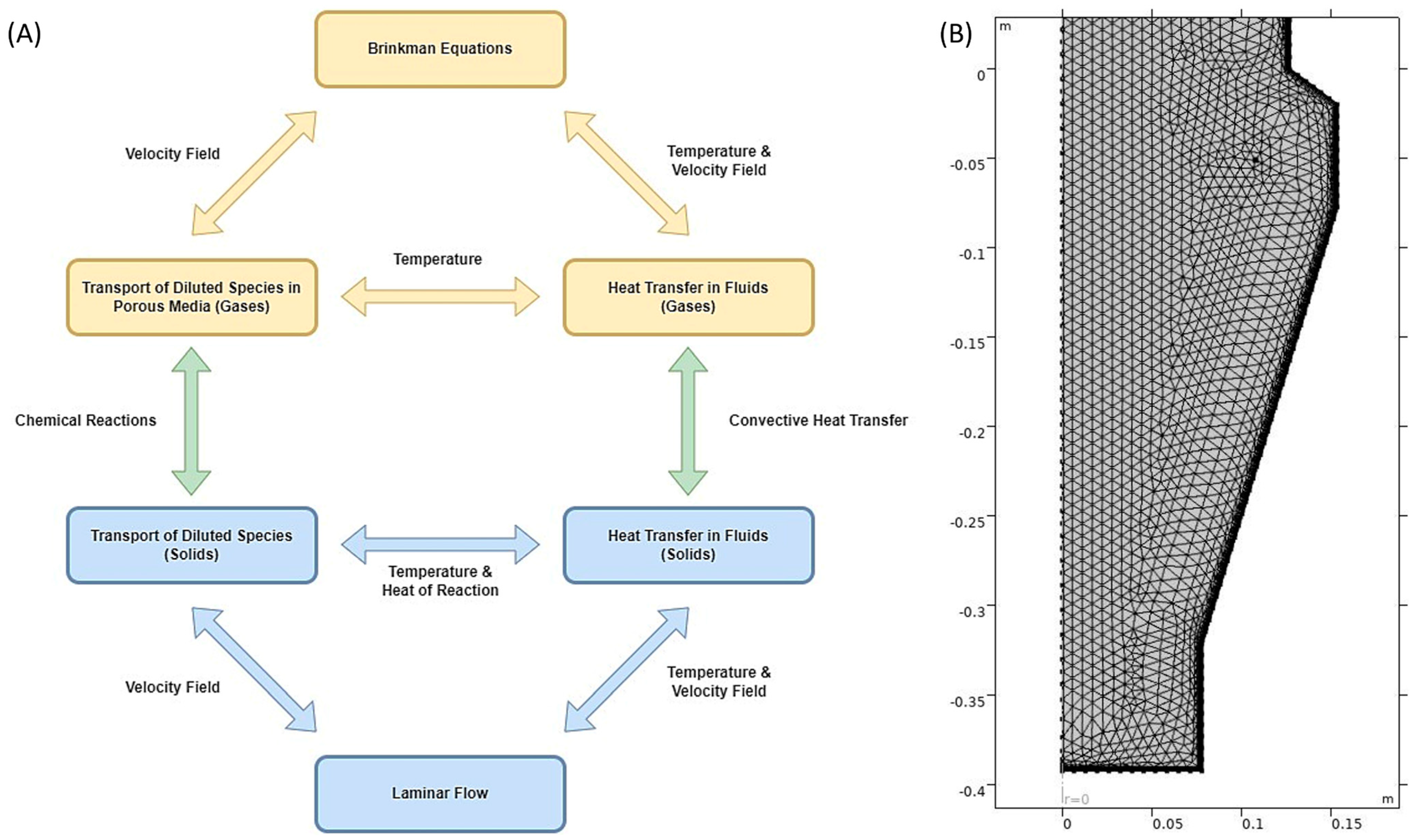
The solid and gaseous phase physics interfaces were interconnected to each other using the Multiphysics coupling, as shown in
Figure 5A. To sum up, the pellets enter the model geometry from the top of the reactor (
Figure 4: boundary 1) and exit at the bottom (
Figure 4: boundary 8). The velocity and pressure field of the solid phase is calculated using the ‘Laminar Flow’ interface, which is coupled with the ‘Heat Transfer in Fluids’ interface via ‘Non-isothermal Flow’ Multiphysics to determine the heat transfer in the solid phase dependent on the velocity field as per Equation (7). The ‘Laminar Flow’ interface is also coupled with the ‘Transport of Diluted Species’ interface using the ‘Reacting Flow’ Multiphysics to determine the reaction rates dependent on the velocity field as shown in Equation (4). Further, the ‘Transport of Diluted Species’ interface is coupled with the ‘Heat Transfer in Fluids’ interface via a common temperature variable for the solid phase, which determines the local heat consumption for the endothermic reactions along with convective heat transfer from solid to gas or vice-versa as per the heat transfer coefficient calculated in Equation (25). The local chemical reaction rate constants are also calculated using the local temperature of the solid phase as per Equation (26).
The inlet gas mixture enters the model geometry from the bustle at the bottom of the reactor (
Figure 4: boundary 4) and exits at the top (
Figure 4: boundary 1). For the gaseous phase, the ‘Brinkman Equations’ interface is used which gives the velocity and pressure field for fluids flowing in a porous media. The ‘Brinkman Equations’ interface is coupled with the ‘Heat Transfer in Fluids’ interface via ‘Non-isothermal Flow’ Multiphysics to determine the heat transfer in the gaseous phase dependent on the velocity field as per Equation (13). The ‘Brinkman Equations’ interface for the gas phase velocity field is also coupled with the ‘Transport of Diluted Species’ interface using the ‘Reacting Flow’ Multiphysics to determine the reaction rates dependent on the velocity field, as shown in Equation (10). Further, the ‘Transport of Diluted Species’ interface is coupled with the ‘Heat Transfer in Fluids’ interface via a common temperature variable for the gas phase, which determines the local convective heat transfer from gas to solid or vice-versa as per the heat transfer coefficient calculated in Equation (25). Equation (25) uses the velocity field obtained from ‘Brinkman Equations’ to calculate Reynold’s number and Prandtl’s number.
As shown in
Figure 5A, the local convective heat transfer, along with the local chemical reaction rates, interconnect the solid and gaseous phases using the local temperature variables and the local concentration variables for both solid and gaseous phases.
4.8. Mesh and Finite Element Solver
To solve the finite element model, the mesh was custom-built, and it was calibrated for fluid dynamics with a normal mesh size. The maximum element size was 0.00691 m, minimum element size was 3.07 × 10
−4 m, maximum element growth rate was 1.15, curvature factor was 0.3, and resolution of narrow regions was 1. The mesh at the boundary layers was handled using splitting at sharp corners of the geometry with a minimum angle of splitting as 240°, a maximum angle per split of 100°, and a maximum of 2-layer decrement. The number of boundary layers in the mesh was 6, and the boundary layer stretching factor was 1.2 with a thickness adjustment factor of 1.
Figure 5B gives a schematic of meshing in the reactor geometry domain.
The model was solved using a segregated solver assuming a steady state. The segregated solver solved the differential equations for each physics interface separately.
5. Model Results and Its Comparison with Pilot Plant Data
The 2D-Axisymmetric model built in this study is capable of predicting the concentration profiles of gases as well as the mass fraction profiles of the solid species along with average metallization at the outlet after accounting for the assumptions. The model is also able to approximately predict the temperature profile and the transition zones for solid species inside the reactor as per the two-step reaction model by Hara et al. [
39].
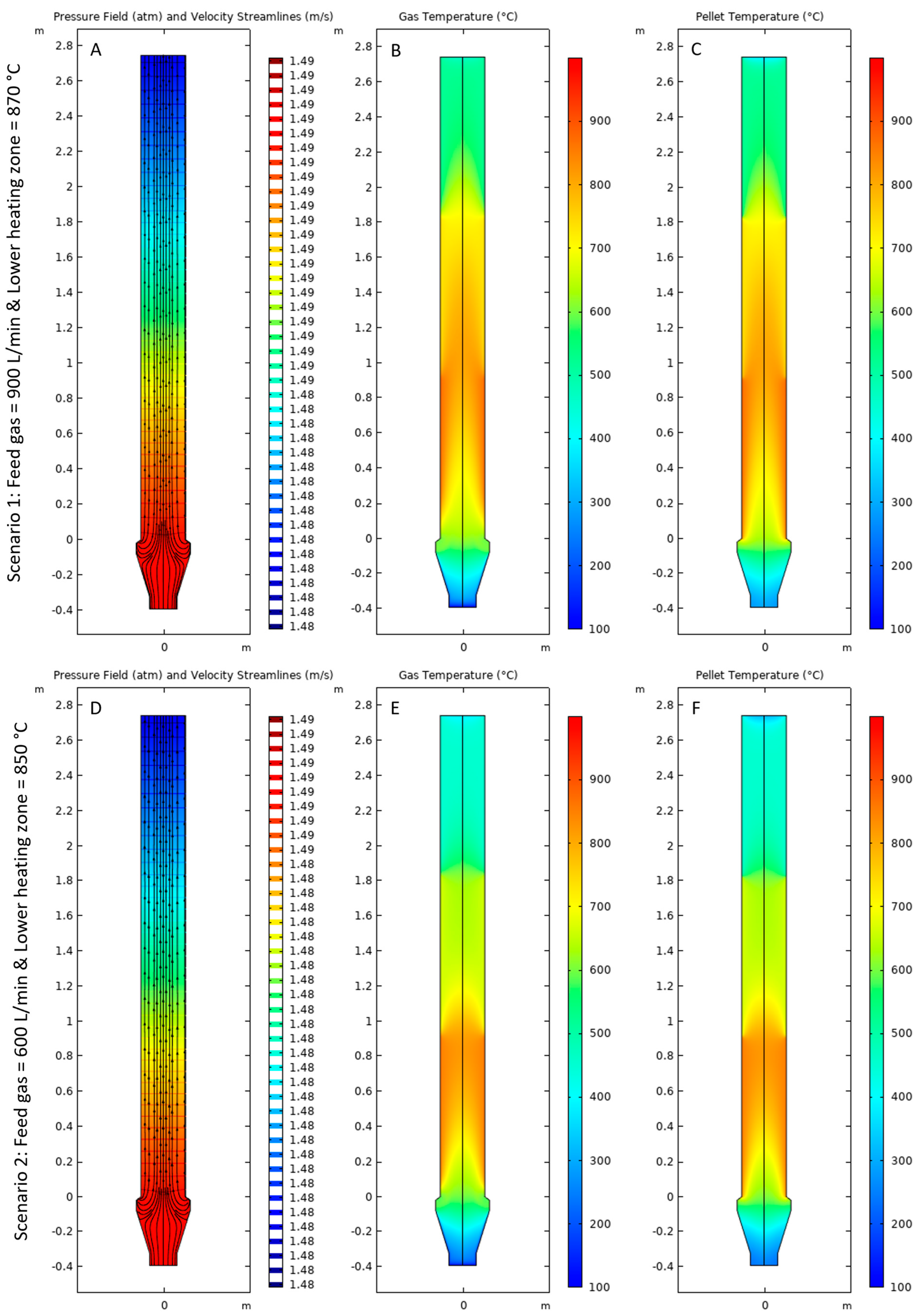
Figure 6A,D shows the pressure field of gases along with their velocity streamlines inside the reactor obtained from solving the Brinkman equations. It can be observed that there was a pressure drop of approximately 0.01 atm from the point of the gas inlet to the point of the gas outlet. The velocity streamlines for the flow of gas appear to diverge from the gas inlet towards the center of the reactor and then move upwards towards the outlet in the direction of the pressure drop.
Figure 6B,C shows the temperature distribution inside the reactor for the gas mixture and the pellet bed, respectively, for Scenario 1. It was observed that the temperature profiles inside the reactor for gases and pellets were very similar due to the thermal equilibrium at the steady state. The temperature of the gas mixture was cooler than the pellet bed at the end of the gas inlet bustle because of the inflow of a small amount of cooling gas. Similar trends in temperature distribution inside the reactor for the gas mixture and the pellet bed were observed for Scenario 2 in
Figure 6E,F. For Scenario 1, the maximum temperature of the gas mixture was observed to be 866.85 °C, and it was 870 °C for the pellet bed in the region near the bottom heating zone. The minimum temperature of the gas mixture was observed to be 28.43 °C, whereas it was 276.52 °C for the pellet bed in the region near the bottom of the gas inlet bustle. For Scenario 2, the maximum temperature of the gas mixture was observed to be 848.52 °C and it was 850 °C for the pellet bed also in the region near the bottom heating zone. Similar to Scenario 1, for Scenario 2, the minimum temperature of the gas mixture was observed to be 24.27 °C, whereas it was observed to be 235.41 °C for the pellet bed in the region near the bottom of the gas inlet bustle.
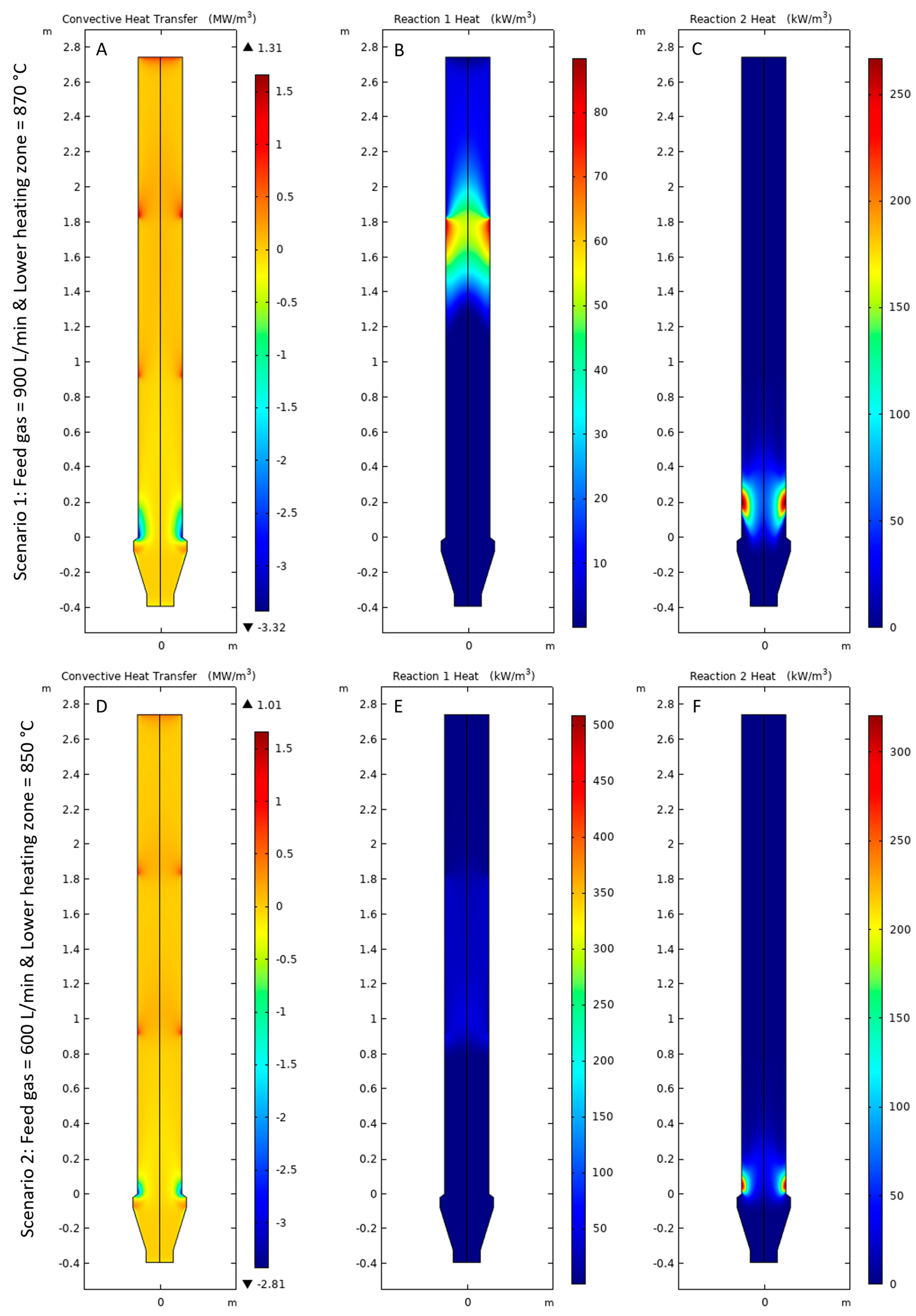
Figure 7A,D shows the convective heat transfer from gas to pellets, it can be observed that the gas quickly loses heat upon entering the bustle inlet due to the temperature difference and the endothermic reaction for both Scenarios 1 and 2. However, as the gas travels upwards, it becomes heated by the pellet bed or achieves a thermal equilibrium with no heat transfer.
Figure 7B,E shows the heat consumed for the conversion of hematite to wüstite for Scenarios 1 and 2, respectively. For Scenario 1, the magnitude of heat consumption was observed to be higher because of higher temperatures in the reaction zone and higher rate of reactions; for Scenario 2, a lower magnitude of heat consumption was observed due to lower temperature in the reaction zone and lower flow rate of H
2 in the gas feed (600 L/min).
Figure 7C,F shows the heat of consumption for conversion of wüstite to iron. The magnitude of heat consumption was higher near the reactor walls than at the center of the reactor. This may occur due to the higher temperatures near the reactor walls compared with the center of the reactor. Further, Scenario 1 consumed more heat than Scenario 2 for the conversion of wüstite to iron because of higher operating temperatures and higher flow of inlet gas (900 L/min).
The gradients in the temperature profiles of gas and pellets in
Figure 6 can be explained by the heat consumption of reaction 1 heat and reaction 2, as shown in
Figure 7. Since both reactions are endothermic, energy was consumed, and a temperature gradient was formed in the region where both reactions took place. Hence, the energy consumption due to the endothermic reactions in
Figure 7B,C,E,F can be correlated to the temperature gradients observed in
Figure 6A,C,E,F.
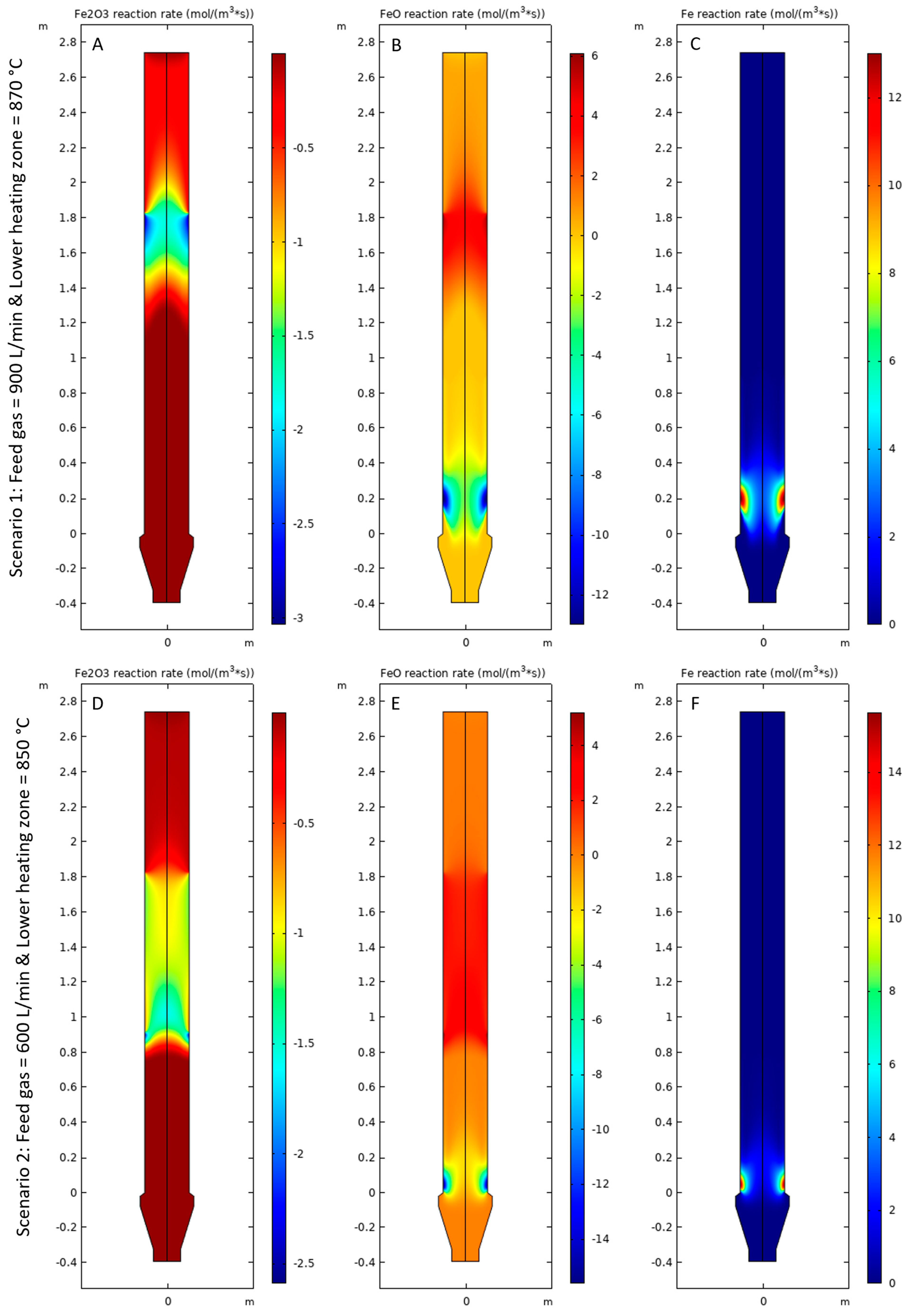
Figure 8A,D shows the rate of consumption of Fe
2O
3,
Figure 8B,E shows the rate of formation and consumption of FeO, and
Figure 8C,F shows the rate of formation of Fe for Scenarios 1 and 2, respectively. It was observed that the magnitude of the rate of reactions was higher for Scenario 1 compared with Scenario 2 due to high operating temperatures and availability of H
2 for the reduction reactions. It was observed that Fe
2O
3 is consumed as the first step of the reaction in a zone approximately between 1.2 m and 1.8 m above the gas inlet bustle at a steady state as shown in
Figure 8A,D. The length of the reduction zone for Scenario 2 appeared to be longer than Scenario 1 due to the lower magnitude of the rate of reduction. In this region, FeO is formed as the product of the first step. As the pellet moves downwards, the mass fraction of FeO increases, as shown in
Figure 9B,E. Approximately 1 m above the gas inlet bustle, FeO starts to reduce to form Fe at a steady state for Scenario 1, as shown in
Figure 8B,C. For Scenario 2, the reduction of FeO starts at approximately 0.4 m above the gas inlet bustle as shown in
Figure 8E,F. The rate of reduction of FeO was higher near the reactor walls compared with the center of the pellet bed for both Scenarios 1 and 2 because the amount of heat available for the endothermic reaction was higher near the reactor walls compared with the region at the center of the pellet bed.
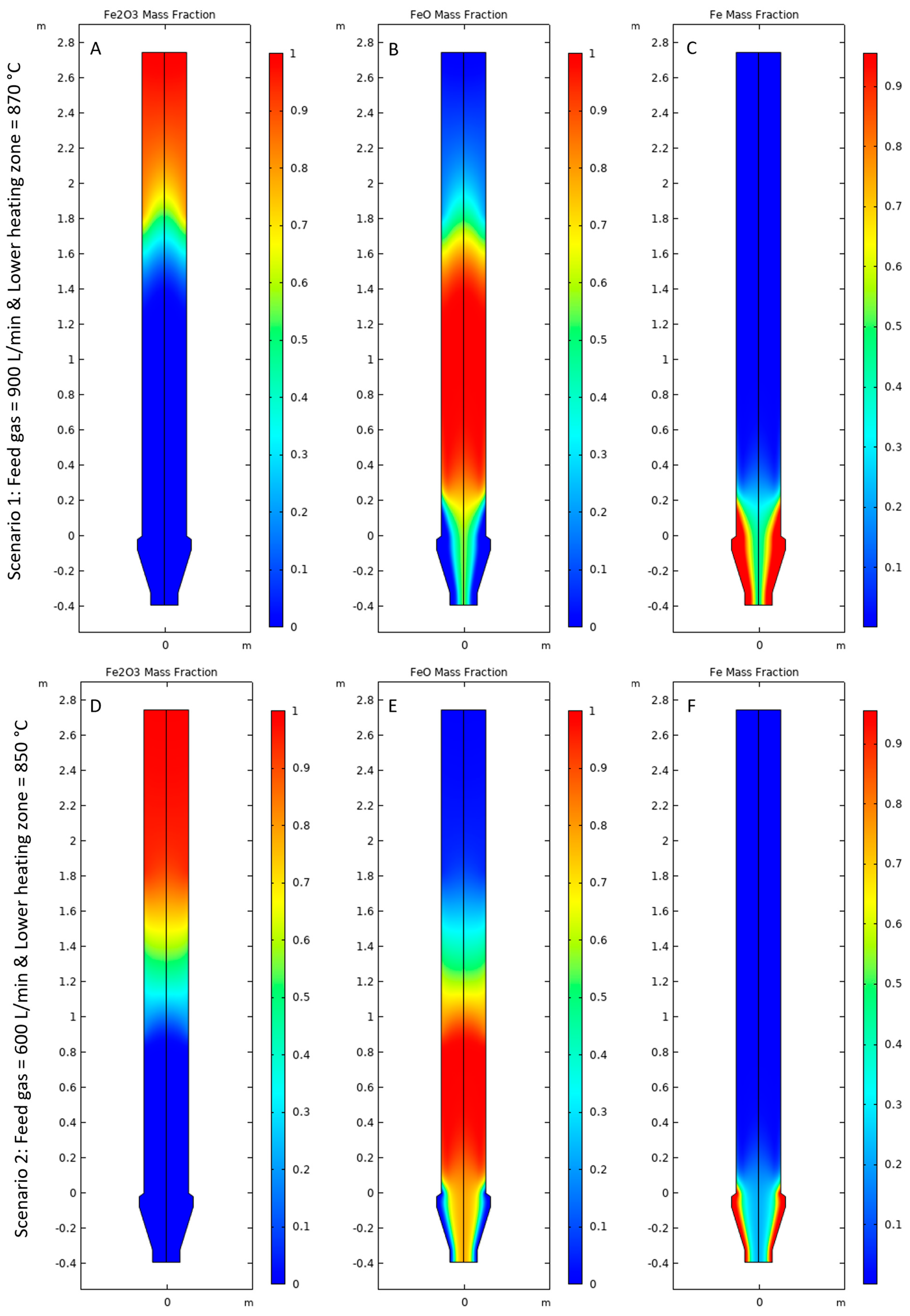
Figure 9A–C shows the mass fractions of all the solid species for Scenario 1 and
Figure 9D–F for Scenario 2. Fe
2O
3 was observed mostly in the upper region of the reactor for both Scenarios 1 and 2, as shown in
Figure 9A,D, respectively. FeO was observed in the middle and lower region of the reactor as per
Figure 9B,E; while Fe was mostly observed in the lower region of the reactor and the gas inlet bustle as shown in
Figure 9C,F. The mass fraction profiles, and the transition gradients can be correlated to the reaction rates of each solid species, as shown in
Figure 8A–F.
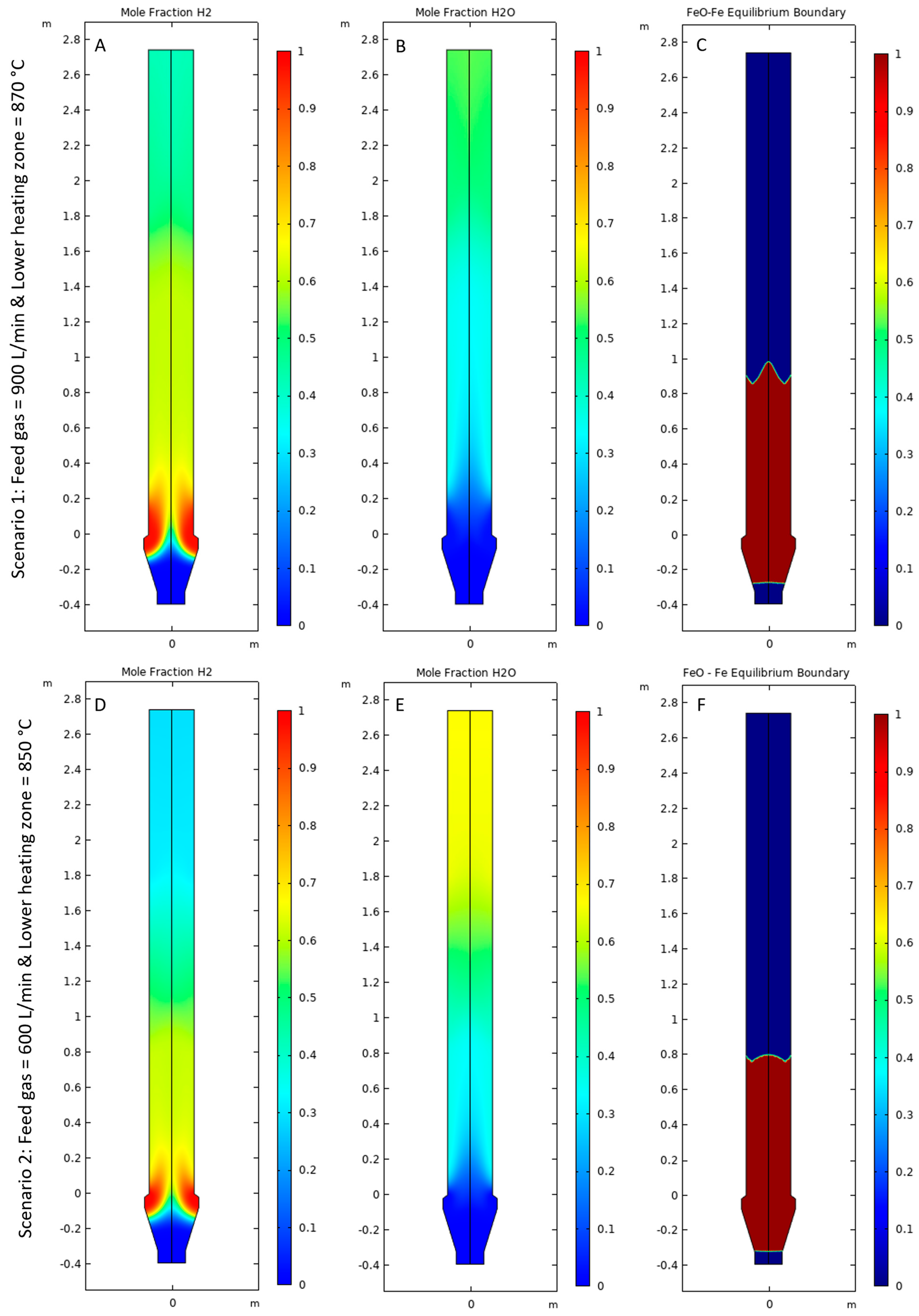
The mole fraction of H
2 and H
2O is shown in
Figure 10A,B for Scenario 1 and
Figure 10D,E for Scenario 2. The mole fraction of H
2 was observed to be very high (~1) for both scenarios in the bottom of the lower heating zone near the reactor walls. As H
2 travels upwards, it is consumed by the FeO to Fe reaction, forming H
2O as a byproduct, which decreases the H
2 mole fraction to approximately 0.6–0.7, while the H
2O mole fraction increases to approximately 0.3–0.4. As H
2 reaches the first reaction zone where Fe
2O
3 is converted to FeO, the mole fraction of H
2 decreases to approximately 0.4–0.5, and the mole fraction of H
2O increases to approximately 0.5–0.6 because of the consumption of H
2 and production of H
2O. The mole fraction of H
2 decreases at a distance of about 1.6–1.8 m from the bottom of the reactor for Scenario 1, while it starts to decrease at a height of 1–1.2 m for Scenario 2 because of the higher rate of reaction in Scenario 1 compared with Scenario 2.
Figure 10C,F show the Fe-FeO Baur–Glässner equilibrium profile for Scenarios 1 and 2, respectively [
10]. The red color indicates the equilibrium moving forward and the formation of Fe, while blue indicates the region where the equilibrium shifts backward, forming FeO. It was observed that the equilibrium shifts backward in the gas inlet bustle for both scenarios because of a drop in temperature and a high mole fraction of H
2O. The equilibrium shifted backward in both the upper and middle regions of the reactor for both Scenarios 1 and 2 because of the higher H
2O mole fraction.
To validate the model, the average metallization at the outlet boundary was also compared with metallization data obtained from the pilot plant trials using the ISO 16878:2016 and ISO 2597-2:2019 methods, as shown in
Table 5. For Scenario 1, the average metallization of the model was 90.9% compared with the 91.8% average metallization obtained from data from the pilot plant trials. For Scenario 2, the average metallization of the model was 65.6% compared with 67.8% obtained from the pilot plant.
Table 5 also shows the comparison of the average temperature observed by the sensors inside the pilot plant reactor vs. the temperature obtained from the model. The difference between the pilot plant temperature profile and the model profile was less than 53 °C for the lower four sensors (S-3 to S-6) for Scenario 1. A large deviation of more than 100 °C was observed for the top two sensors (S-1 and S-2). Similarly, for Scenario 2, the difference between the pilot plant temperature profile and the model profile was less than 68 °C for the lower four sensors (S-3 to S-6), and a large deviation of more than 100 °C was observed for the top two sensors (S-1 and S-2). This may be caused by the assumption that the thermal expansion of the rod on which the sensors are mounted is negligible, along with the two-step reaction approximation, which ignores the thermal conductivity of magnetite.
Compared with the previously reported studies on reactor models for ironmaking using a direct reduction process, the current study reports the average metallization along with the internal temperature profile of the reactor. The model has also been validated for very low metallization, which has not been reported in previous studies. Hamadeh et al. reported a model that predicts the metallization, composition of pellet, and outlet gas composition, but it does not report the validation of the model using internal temperature profiles and operation of the model at lower metallization [
29]. Ghadi et al. reported a model for the Midrex shaft reactor that only focused on gas flow and lacked the comparison of model results with reactor data, such as the internal temperature profile of the pellet bed and metallization of pellets [
30]. The model reported in this study is able to fill these knowledge gaps. However, the model needs further improvement by considering the three-step conversion from hematite to iron instead of the two-step conversion, along with improving the heat balance through the reactor walls and the addition of the more complicated physics. A more complex model can be made by using the physics of solid flow for the moving pellets instead of assuming the flow of pellets as a fluid flowing in a laminar regime in a 3D geometry. Future studies will be focused on building a mixed gas model and obtaining pilot plant trial data for hydrogen and natural gas mixture as reducing agents.


 ,
, 


