Article

Prediction of Surface Location Error Considering the Varying Dynamics of Thin-Walled Parts during Five-Axis Flank Milling

1
State Key Laboratory for Manufacturing Systems Engineering, Xi’an Jiaotong University, Xi’an 710054, China
2
AVIC Xi’an Aircraft Industry Group Company Ltd., Xi’an 710089, China
*
Author to whom correspondence should be addressed.
Processes 2023, 11(1), 242; https://doi.org/10.3390/pr11010242
Submission received: 16 December 2022 / Revised: 8 January 2023 / Accepted: 9 January 2023 / Published: 11 January 2023
(This article belongs to the Special Issue High-Performance Machining Processes: From Mechanisms to Equipment)

Abstract

:
Surface location error (SLE) caused by forced vibration is a key factor to determine the quality of the finished part. When machining thin-walled structures with sculptured surfaces, the complicated milling process is significantly influenced by the vibration due to the flexibility of the part. The dynamics of the part are dominant and vary with the material removal during machining. This paper presents a prediction method of SLE considering the varying dynamics of thin-walled parts in five-axis flank milling. The in-process part is decomposed into unmachined and machined portions, which are both modelled based on the thin-plate theory. The dynamics models of the two portions are coupled using the substructure method. Coordinate transformation based on the screw theory and the general cutting dynamics model for five-axis flank milling is employed to transform the cutting force vectors and frequency response function (FRF) to the same coordinate system for the prediction of SLE. The proposed method is validated with five-axis flank milling tests and SLE measurements on a thin-walled twisted part. It is shown that the average error of the proposed method for SLE prediction is less than 5 μm, and the calculation is almost 8 times faster than the typical finite element method.

1. Introduction

Thin-walled parts with sculptured surfaces are widely used in the aerospace industry, which are always machined through five-axis flank milling. These parts normally contain thin walls (1.5–4 mm thickness) and require good surface quality. Forced vibration induced by the flexibility of parts is a significant factor influencing the dimensional quality of the parts [1], which significantly affect their service performance [2]. The prediction of surface location error (SLE) of thin-walled parts represents the basis of determining the proper cutting parameters, which aims at increasing the productivity and reducing the costs of a milling operation [3]. However, the varying dynamics of the part during machining and the complexity of the milling process both increase the difficulty of SLE prediction.
The prediction of SLE is based on the dynamics of the part. Li [4] and Ismail [5] employed experimental modal analysis (EMA) to measure the dynamics of flexible parts. However, the material of the part is removed during machining, and the dynamics of the part vary with this process. Finite element (FE) models are employed to predict the dynamics of a part to avoid the interruption of the machining process caused by EMA. Tsai et al. [6] and Adetoro et al. [7] employed the FE model to analyze the deflection of a thin-walled part during machining, and pointed out that the dynamics of the part influenced the machining process significantly, whereas with the rapid development of industries, the dimension of parts becomes larger and the element’s number of the corresponding FE model is huge, which is time-consuming for dynamics prediction. Thus, computationally efficient methods simplified by either elements [8] or computational processes [9,10] are proposed to solve pertinent problems. Meshreki et al. [11] presented a dynamics model based on Rayleigh’s energy method to reduce computational time for thin-walled pockets; then, they [12,13] updated the model to take into account the continuous changes in the part’s thickness. Tuysuz et al. [14,15] used reduced-order substructure and perturbation methods to further improve the efficiency of computing dynamics for thin-walled parts in milling. Ma et al. [16] proposed a method to predict the dynamics of thin-walled parts based on the equivalent plate and the external damping effect. However, the major puzzle in simulation is the contradiction of efficiency, accuracy, and convenience [17], and it is hard to offer the efficiency to compute dynamics and the versatility to model parts with complex geometries simultaneously.
The relationship between the machining quality and process was investigated by Kline [18], Tlusty [19], and Sutherland [20] early, and then Schmitz et al. [21] studied the prediction method of SLE systematically based on the frequency response function (FRF) of a tool tip. However, in the milling of thin walls, the flexibility of the parts determines the SLE of the finished parts. Some scholars studied the surface quality based on thin plates. Altintas et al. [22] predicted surface errors based on the dynamics model of a cantilever plate structure and pointed out that the dynamics of a part are dominant in the flank milling of thin-walled structures. Budak et al. [23] modelled the milling process of cantilevered plates, and showed that the vibration between the part and cutter influences the surface quality of the part significantly. Ratchev et al. [24] predicted surface errors caused by the deflection of low-stiffness parts through an adaptive flexible theoretical deflection model. Moreover, Sofuoglu et al. [25] developed regression–multicriteria decision-making hybrid models and determined the optimum cutting conditions without chatter vibrations. Li et al. [26] divided the factors determining machining quality into kinematic and stochastic portions. Misaka et al. [27] predicted surface roughness by integrating the data obtained through an experiment and an analytical model to improve computational efficiency. Meanwhile, Ringgaard et al. [28] demonstrated that the relative forced vibration between the tool and the part must be minimized to improve the machining quality. Jiao et al. [29] developed a surface roughness model considering the forced vibration in two directions. Li et al. [30] proposed a prediction model of deformation induced by cutting forces based on the substructure method for the thin-walled parts in flank milling. Other scholars predict SLE with the consideration of tool and part deflection [31], process damping [32], tool dynamic stiffness variation [33], etc. However, past prediction methods have mainly been based on simple cutting conditions. A huge gap still exists between reality and simulation due to the limitation of computational efficiency and simplified models [34]. The SLE prediction method of thin-walled parts with the consideration of varying dynamics in five-axis flank milling has not been reported in the literature.
A prediction method of SLE considering the varying dynamics of thin-walled parts during five-axis flank milling is proposed in the paper. The in-process part is represented by the machined and unmachined portions, and the substructure method is employed to couple the dynamics model of two portions, as presented in Section 2. The SLE of thin-walled parts in five-axis flank milling is predicted in Section 3 based on the developed dynamics model and screw theory. The proposed method is verified in Section 4. Section 5 concludes the paper.

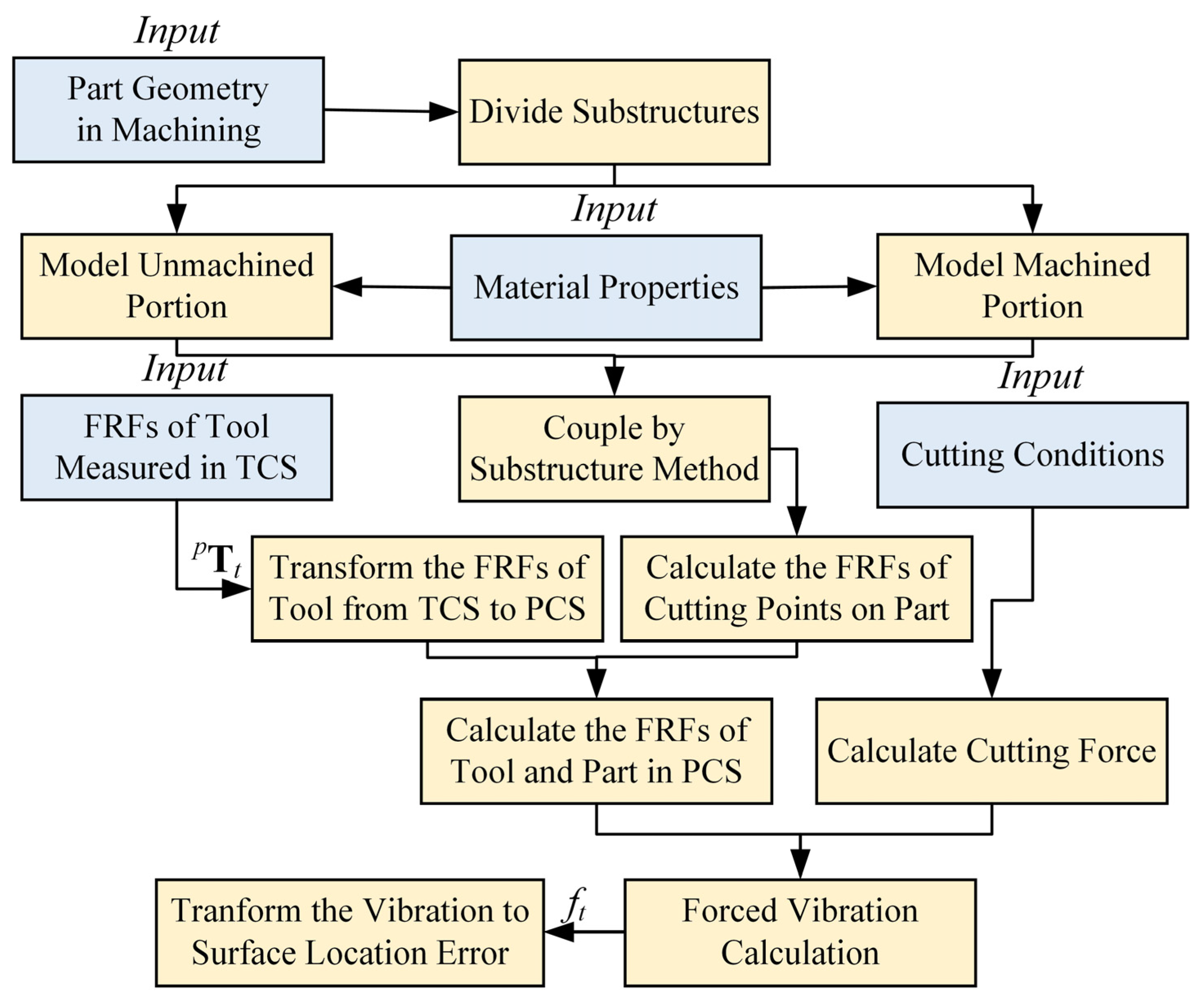
2. Dynamics Model of Thin-Walled Part during Milling

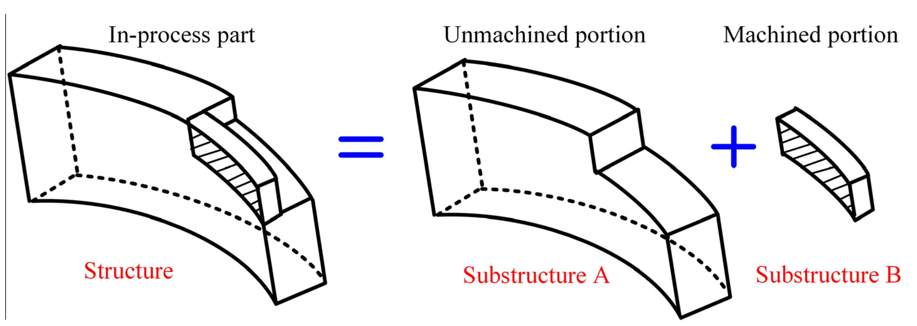
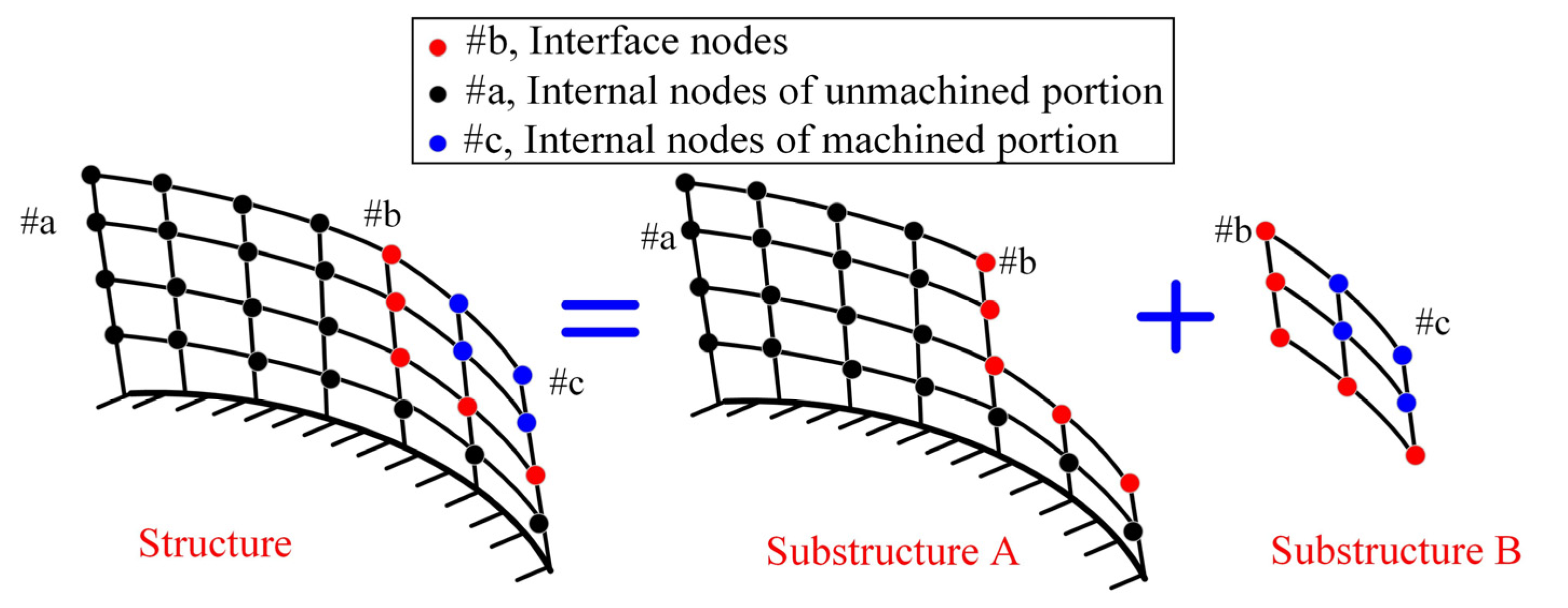
2.1. Machined and Unmachined Portions of In-Process Part

The in-process part is composed of unmachined and machined portions. The thickness of the machined portion is smaller than the unmachined portion. The prediction of SLE depends on the FRFs of the cutting point on the part, which is determined by the dynamics of two portions. The decomposition of the in-process part is illustrated in Figure 1.
The machined and unmachined portions are regarded as substructures of the in-process part. The dynamics model of the in-process part ([ Θ ]) is obtained by coupling the dynamics of two substructures, expressed by
Θ = Θ u n + Θ m a
where [ Θ un] and [ Θ ma] represent the dynamics of the unmachined and machined portions of the part, respectively.

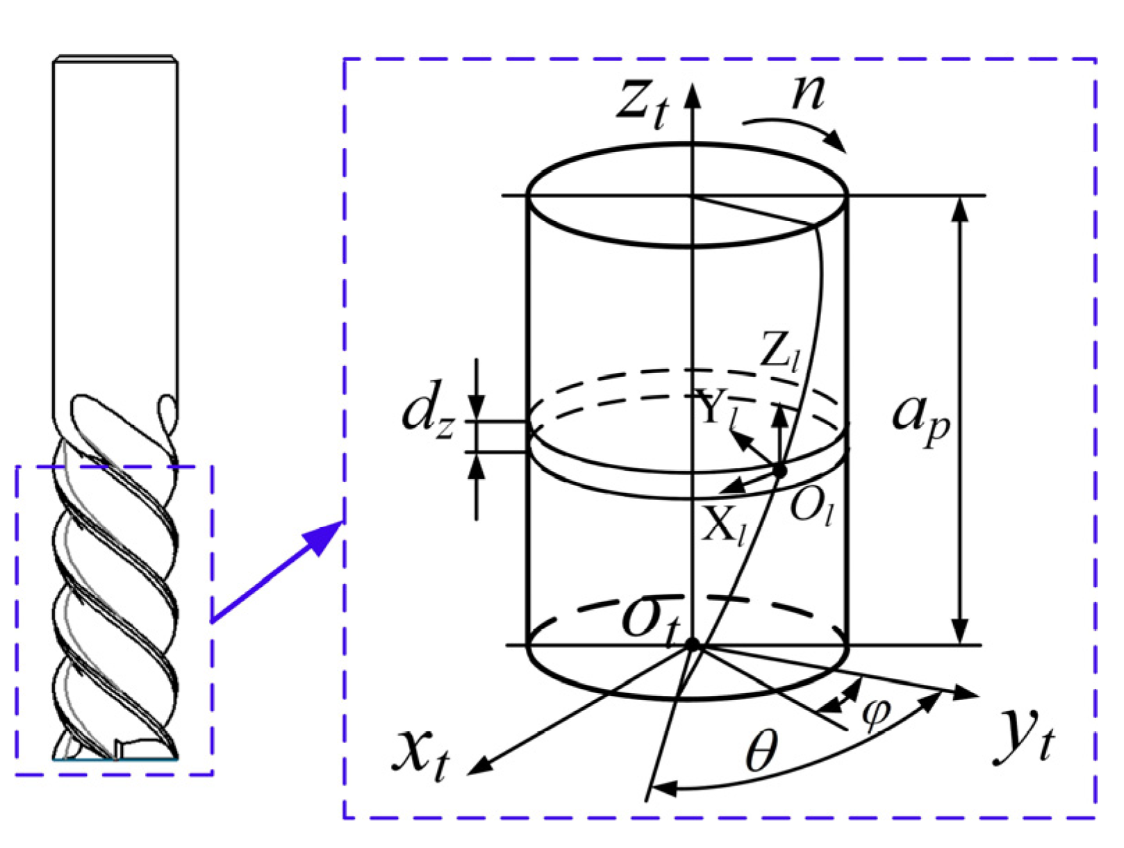
2.2. Dynamics Model of Thin Wall

For thin-walled parts, the thickness is so small compared to the length and height. Therefore, in the thickness direction, the value of stress can be regarded as constant. The part is represented by the neutral plane, and it is meshed by the appropriate elements. Each node of the element contains three degrees of freedom (DOF) based on Kirchhoff’s thin-plate theory. The virtual work principle is used to develop the stiffness matrix Ke and mass matrix Me of the element, expressed as
M e = S e w τ N T N d S
K e = V e τ 3 B T D B d V
where w is the product of the density of the material and the area of the element. τ is the thickness of the part. N is the shape function depending on the type of element, and B is derived from N. D is the modified bending modulus, calculated by
D = E 12 ( 1 υ 2 ) 1 υ 0 υ 1 0 0 0 ( 1 υ ) / 2
where E is the elastic modulus, and υ is the Poisson’s ratio.
The accuracy of Rayleigh damping is enough for establishing the damping matrix. Meanwhile, the computational efficiency is high. Based on the damping coefficients (α and β), Rayleigh damping is the function of mass and stiffness matrices, given by
C e = α M e + β K e
The matrices of elements are assembled on nodes to comprise the matrices of the part. The dynamics model of a thin wall is expressed as
M X ¨ + C X ˙ + K X = F
where M, C, and K are the mass, damping, and stiffness matrices of the part. X and F are the displacement and force vectors, respectively.

2.3. Coupling Using the Substructure Method

The unmachined and machined portions are defined as substructures of the part, and the dynamics of two portions are coupled by the substructure coupling method. The dynamics model of the substructure is expressed as
M r X ¨ r + C r X ˙ r + K r X r = F r ( r = u n or m a )
where r is un or ma, denoting the unmachined portion and the machined portion, and this notation is used in the following equations. By using the Laplace transform, Equation (7) is transformed into the frequency domain from the time domain.
S r ( ω ) = ω 2 M r + ω C r + K r
where Sr(ω) is the dynamic stiffness matrices of the substructure. [ Θ un] and [ Θ ma] in Equation (1) are rewritten as
Θ r = S r ( ω ) 1
The coupling process of two substructures is shown in Figure 2. The interface nodes and internal nodes of the unmachined portion and machined portion are labelled as #a, #b, and #c. Each node contains three degrees of freedom (DOF) based on the dynamics model of a thin wall developed in Section 2.2.
The dynamic stiffness matrix Sr, in which the ω is dropped for clarity, is rewritten as the matrixes of different DOF sets, populated by
S r = S u n = S u n c c S u n c b S u n b c S u n b b S m a = S m a b b S m a a b S m a b a S m a a a
where the superscripts a, b, and c represent the DOF sets of #a, #b, and #c respectively. The force vector Fr is rewritten as the vector of different DOF sets, expressed by
F r = F u n = F u n c F u n b F m a = F m a b F m a a
The dynamics model of two substructures is composed as
S u n c c S u n c b 0 0 S u n b c S u n b b 0 0 0 0 S m a b b S m a a b 0 0 S m a b a S m a a a X u n c X u n b X m a b X m a a = F u n c F u n b F m a b F m a a
Based on the compatibility of interface displacements, the transformation of DOF vectors from the structure to the substructure is represented by
X u n c = X c X u n b = X b X m a b = X b X m a a = X a I 0 0 0 I 0 0 I 0 0 0 I X c X b X a = X u n c X u n b X m a b X m a a
Based on the force equilibrium, the transformation of force vectors from the substructure to the structure is written as
F u n c = F c F u n b + F m a b = F b F m a c = F m a c I 0 0 0 0 I I 0 0 0 0 I F u n c F u n b F m a b F m a b = F c F b F a
Substituting Equations (13) and (14) into Equation (12) yields
I 0 0 0 0 I I 0 0 0 0 I S u n c c S u n c b 0 0 S u n b c S u n b b 0 0 0 0 S m a b b S m a a b 0 0 S m a b a S m a a a I 0 0 0 I 0 0 I 0 0 0 I X c X b X a = F c F b F a
The dynamic stiffness of structure Sun+ma can be expressed by
S u n + m a = I 0 0 0 0 I I 0 0 0 0 I S u n c c S u n c b 0 0 S u n b c S u n b b 0 0 0 0 S m a b b S m a a b 0 0 S m a b a S m a a a I 0 0 0 I 0 0 I 0 0 0 I
Based on the Equation (16), the dynamics of the in-process part ([ Θ ]) are represented as
Θ = S u n + m a 1
The FRF of the part in the cutting point is calculated by
H p = Θ q = i = 1 n Ψ i q Ψ i q T ( ω i 2 ω 2 ) + 2 j ζ i ω i ω
where q is the DOF in the thickness direction of the cutting point. ωi, Ψiq, and ζi are the eigenvalue, eigenvector, and modal damping ratio calculated from Equation (17), and n′ is the number of natural modes.

3. Prediction of Surface Location Error

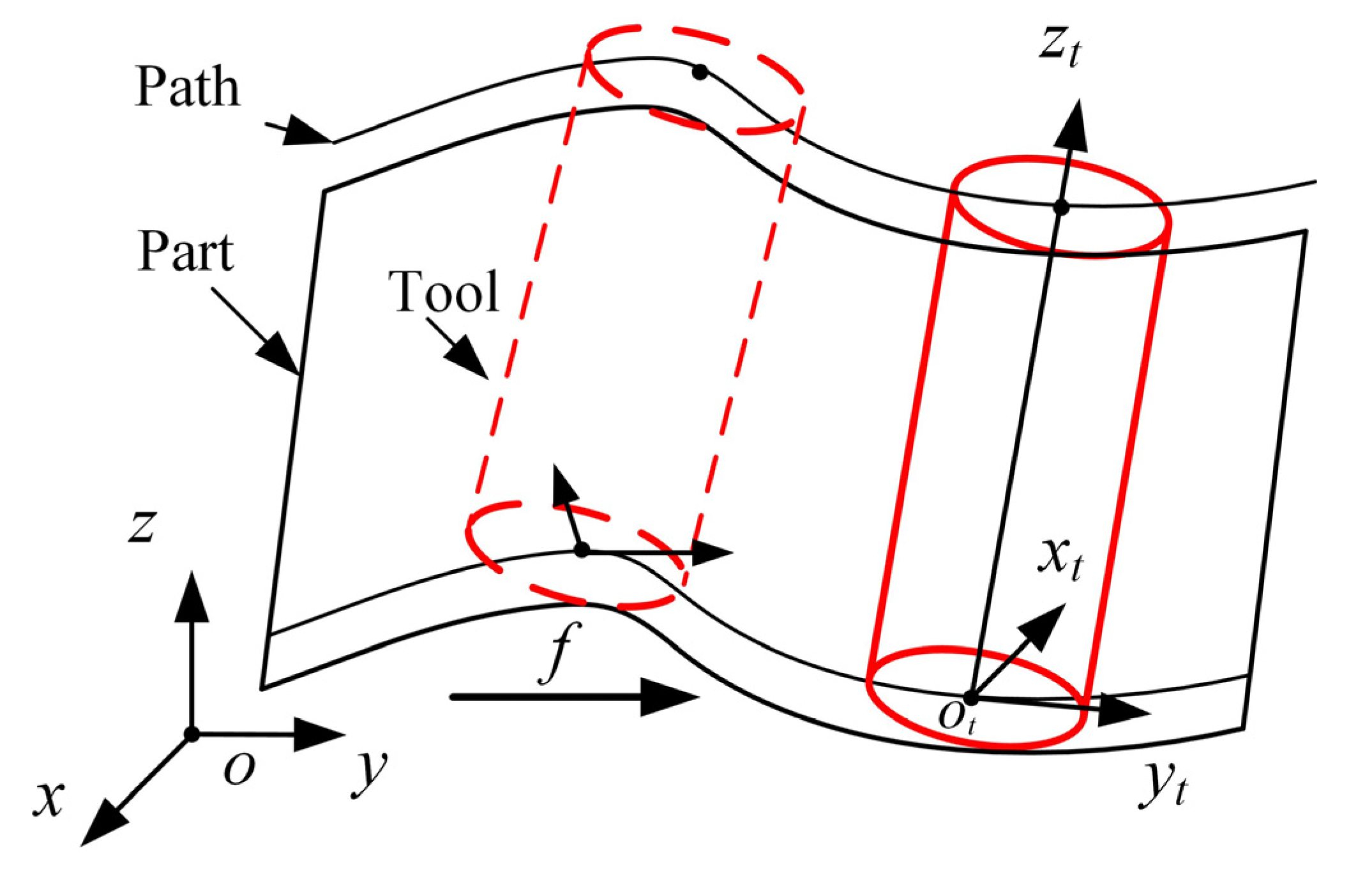
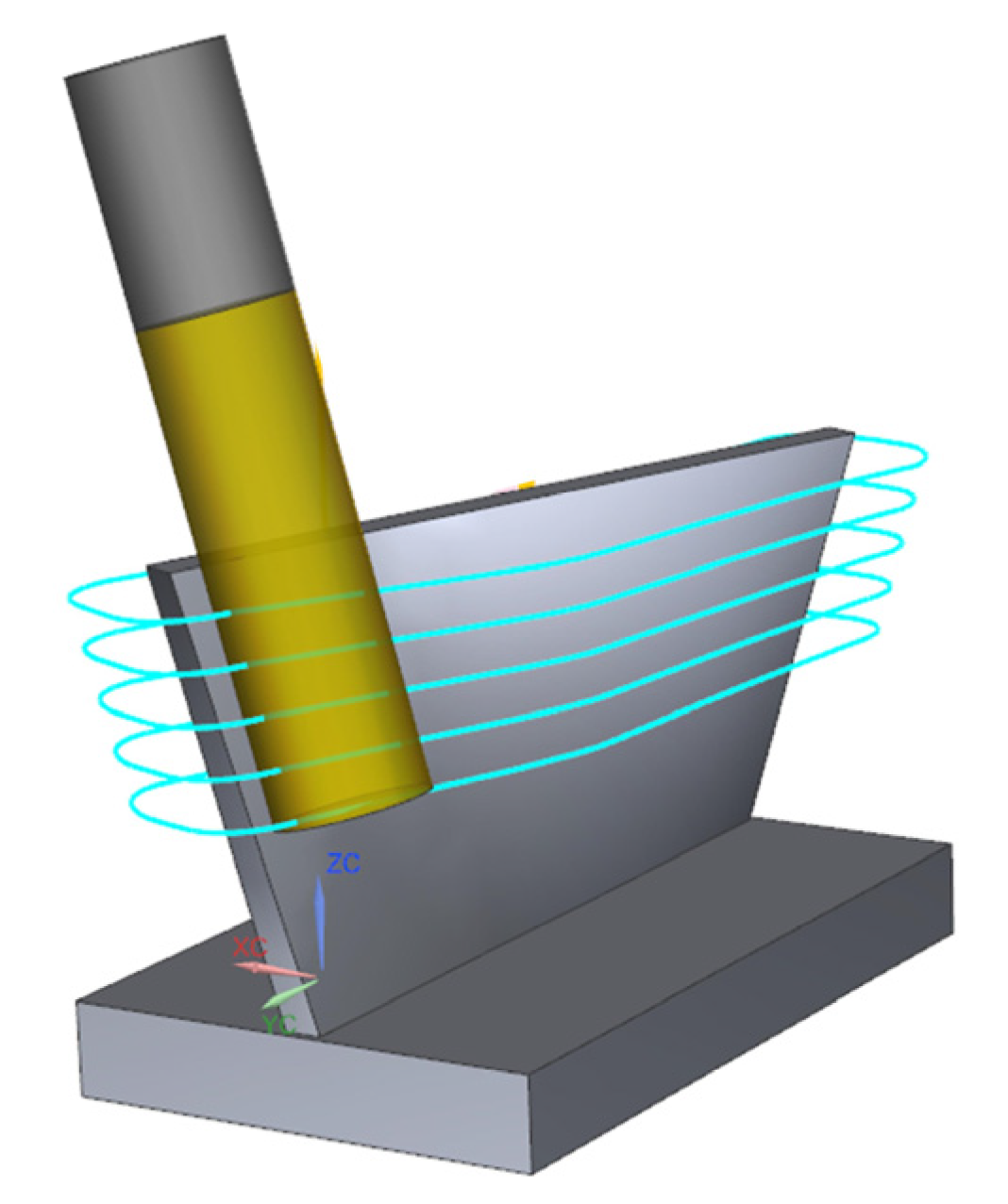
3.1. Coordinate Transformation in Five-Axis Flank Milling Based on Screw Theory

The part coordinate system (PCS) and the tool coordinate system (TCS) are established as illustrated in Figure 3. The FRFs of cutting points on the part are predicted in the PCS, and the TCS is used to analyze the dynamic response of the tool tip. However, the forced vibration should be calculated in the PCS. A simple but efficient method based on the general cutting dynamics model [4] and the screw theory is employed to transform the TCS into the PCS, expressed as
T p t ( θ 1 , θ 2 ) = e s 1 ω 1 θ 1 e s 2 ω 2 θ 2 T p t ( 0 )
where θ1 and θ2 are the rotation angles [35] of two rotary axis in five-axis flank milling. The two rotary axes can be distinguished based on being close to either the part or the tool, and ω1 and ω2 are the unit rotary vectors of the two rotary axes. s1 and s2 are −1 if the rotary axis is mounted on the table side; otherwise, they are 1. pTt (0) is the orientation of the TCS in the PCS at the beginning of machining [36].
The FRF of the tool tip can be transformed in the PCS based on Equation (19), and the FRF in the cutting point is calculated by
H t p = T p t H t T t p + H p
where Ht and Hp are the FRFs of the tool and the part, respectively. Ht can be obtained through modal testing, and Hp is calculated by Equation (18).

3.2. Surface Location Error in Five-Axis Flank Milling

A cutting force is required to predict the SLE. A typical end mill is illustrated in Figure 4. Based on a tiny axial length dz, the cutting portion of the flute is represented by m disk elements. The local coordinate system OlXlYlZl (LCS) is created attached to the cutting edge, where axes Xl, Yl, and Zl are axial, radial, and tangential along the tool as shown in Figure 4.
For the ith element of the jth tooth, the tangential, radial, and axial cutting forces at t time with the rotation angle φi,j(t) are expressed as
d F t = χ ( φ i , j ( t ) ) K tc h ( φ i , j ( t ) ) + K te d z d F r = χ ( φ i , j ( t ) ) K rc h ( φ i , j ( t ) ) + K re d z d F a = χ ( φ i , j ( t ) ) K ac h ( φ i , j ( t ) ) + K ae d z
where K is the cutting force coefficient. The subscript t, a, and r represent the tangential, axial, and radial directions, respectively, and the subscript c and e are employed to distinguish the shear and plow cutting force. h(φi,j(t)) is the chip thickness at t time. χ (φi,j(t)) is employed to determine whether the cutting force is developing, expressed by
χ ( φ i , j ( t ) ) = 1 , θ s t φ i , j ( t ) θ e x 0 , otherwise
where θst and θex stand for the angles of entry and exit, respectively.
The tangential, radial, and axial cutting forces are developed in the LCS, and transformed to in the TCS based on the transition matrix R.
d F x t   d F y t   d F z t = R d F t d F r d F a
R = cos φ sin φ 0 sin φ cos φ 0 0 0 1
The total cutting force in the TCS is calculated by
F t = F x t F y t F z t = j = 1 n i = 1 m d F x   d F y   d F z
where n is the tooth number of the cutting tool. The cutting force is defined in the TCS, but forced vibration displacement is calculated in the PCS, which can be transformed by pTt, expressed as
F PCS ( t ) = T p t F t
The forced vibration displacement is calculated by
X ( t ) = f fourier 1 H t p F PCS ( ω )
where f−1fourier represents the inverse Fourier transformation operator. With the prediction of forced vibration displacement, the SLE at the position of the tool tip on the part can be predicted by
x ( s ) = X s f t
where s is the length of the distance on the part from the cutting beginning to the position of SLE prediction; ft is the feed rate.
The overall procedure is summarized as shown in Figure 5.

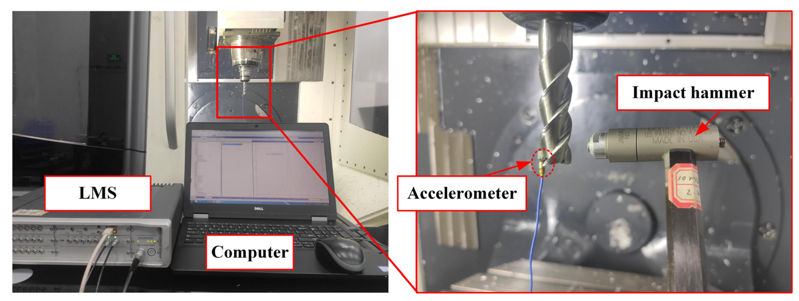
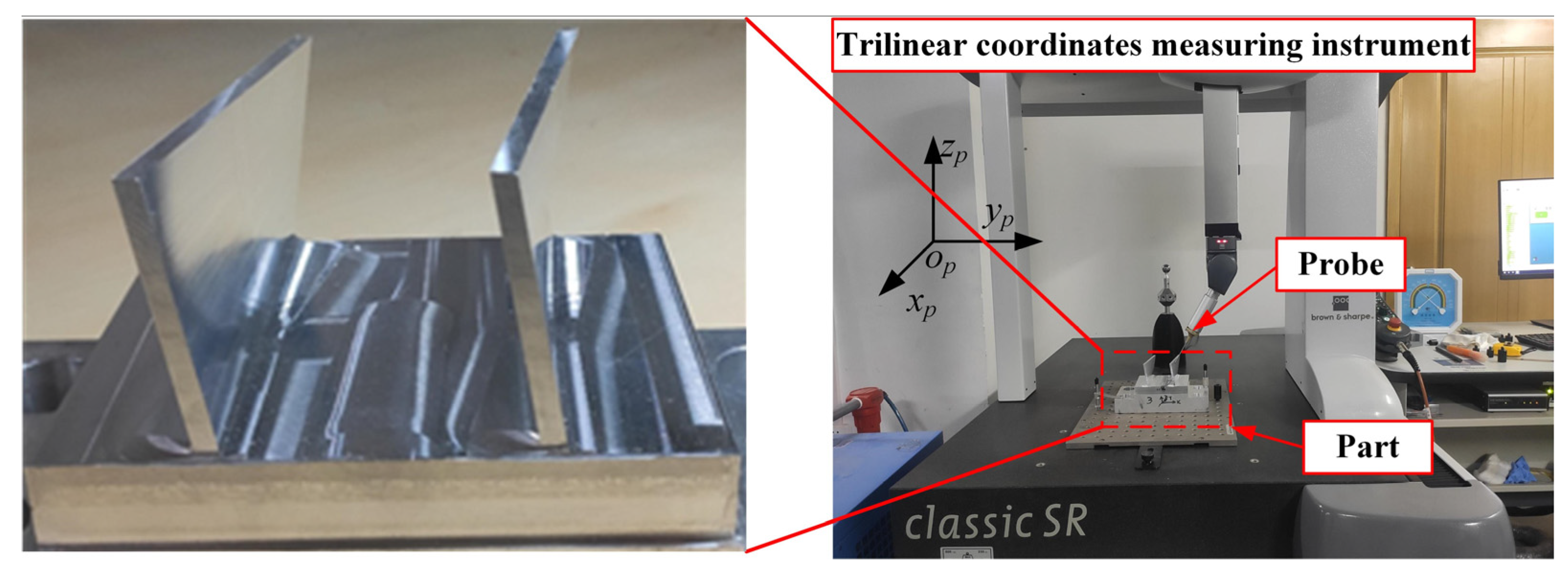
4. Experimental Verification

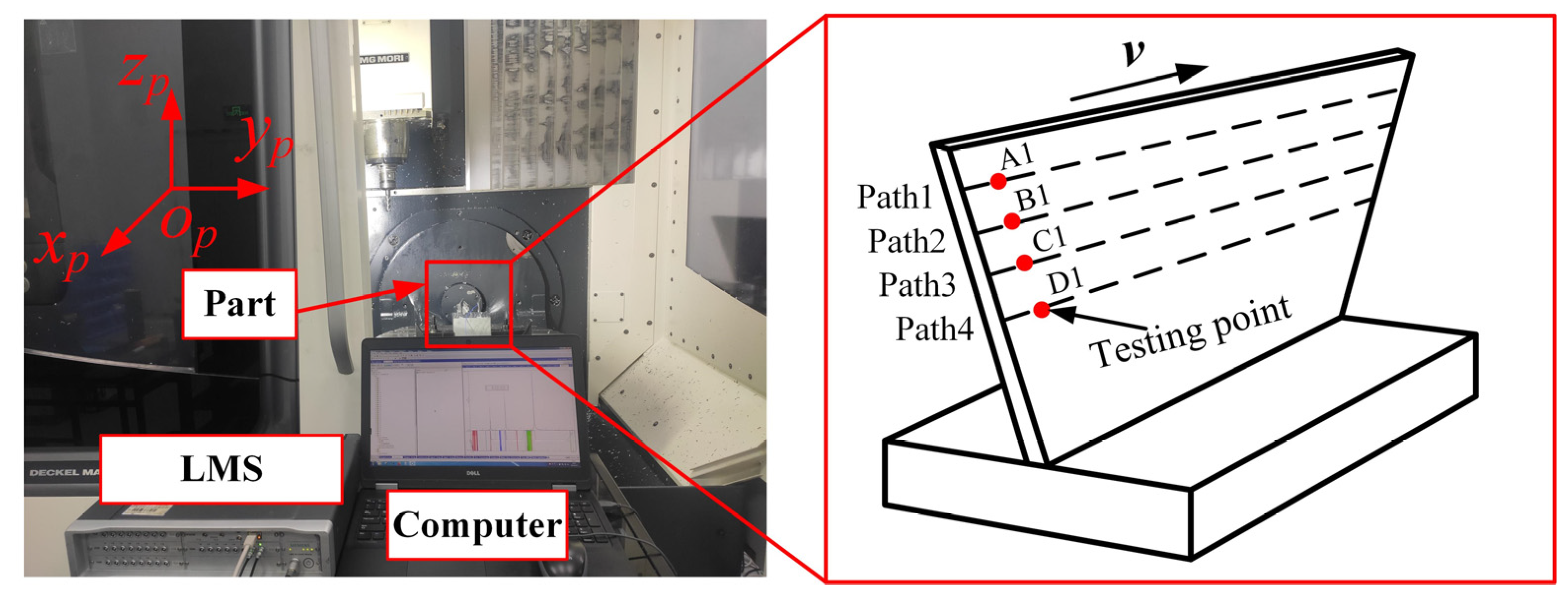
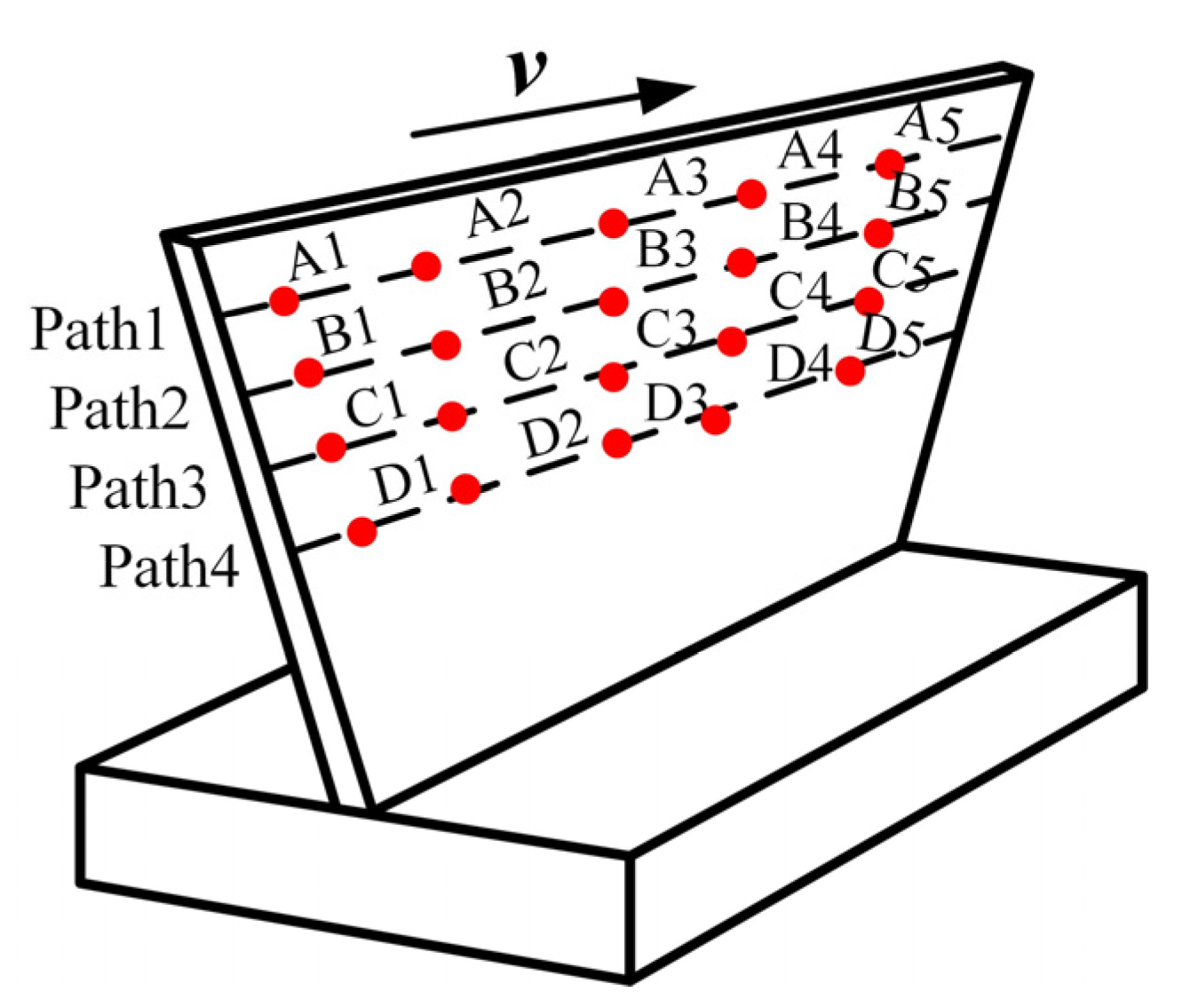
4.1. Experiment Design

A thin-walled twisted benchmark with dimensions of 100 mm × 45 mm × 6 mm was designed to verify the proposed SLE prediction method. The material is Al7075 with the following properties: E = 69 × 109 Pa, μ = 0.3, and ρ = 2750 kg/m3. The α and β, which are the proportional damping constants of the benchmark and identified by experiments, are 0.84 and 5.93 × 10⁻⁸, respectively. The thickness of the benchmark was machined from 6 mm to 4 mm by using flank milling as shown in Figure 6.
The impact testing was used to obtain the FRFs of the tool tip, as shown in Figure 7. The solid carbide end mill with 3 teeth and a diameter of 16 mm was equipped to a five-axis table-tilting machine center (model: DMU50) (DMG MORI, Inc., bielefeld, Germany). The tool tip was impacted by the hammer with the model of PCB 086C03 (PCB Piezotronics, Inc., Depew, NY, USA), and an accelerometer with the model of PCB 352C23 (PCB Piezotronics, Inc., Depew, NY, USA) was employed to obtain the vibration responses. The acquisition system of model LMS SCADA305 (LMS, Inc., Reuven, Belgium) was used to analyze the impact and response data. To reduce the inaccuracy caused by accident, the impact testing was repeated 5 times and the mean value was chosen as the final measured FRFs.
The same experimental setups were also employed to obtain the FRFs of the part during machining. The FRFs of points on the part were different, and the points A1, B1, C1, and D1 with a uniform distance, which equaled the axial depth of the cut to keep the FRF testing only at the position of the tool tip on the part, were chosen for the following experiments. The testing points and the corresponding paths are shown in Figure 8. The testing point A1 was measured without material removal. For other testing points, cutting stopped for FRF measurements after the previous path was finished.
Figure 9 shows the comparison of FRFs between the tool tip and the part, where the dynamics of the part are more dominant. Therefore, only the FRFs of the part were employed to predict the SLE. The radial depth of cut was assigned as 1mm based on the thickness of the benchmark and the axial depth of cut was set to 5 mm. The feed rate was 0.1 mm/tooth. Based on the defined cutting conditions and chatter stability lobes, the chatter-free spindle speed for all four paths was chosen as 6000 rpm.
The SLEs at the position of the tool tip on the part were chosen to be predicted and measured for clarity, and the corresponding paths are illustrated in Figure 8. For the finished part, the SLEs in the four paths were measured by the trilinear coordinates measuring instrument (model: Global Classic SR 05.07.05) (Hexagon AB, Inc., Stockholm, Sweden) as shown in Figure 10. On each path, measuring points were chosen with an interval of 2 mm. Coordinate values on both sides of each point were measured to calculate the SLEs by comparing with the part model.

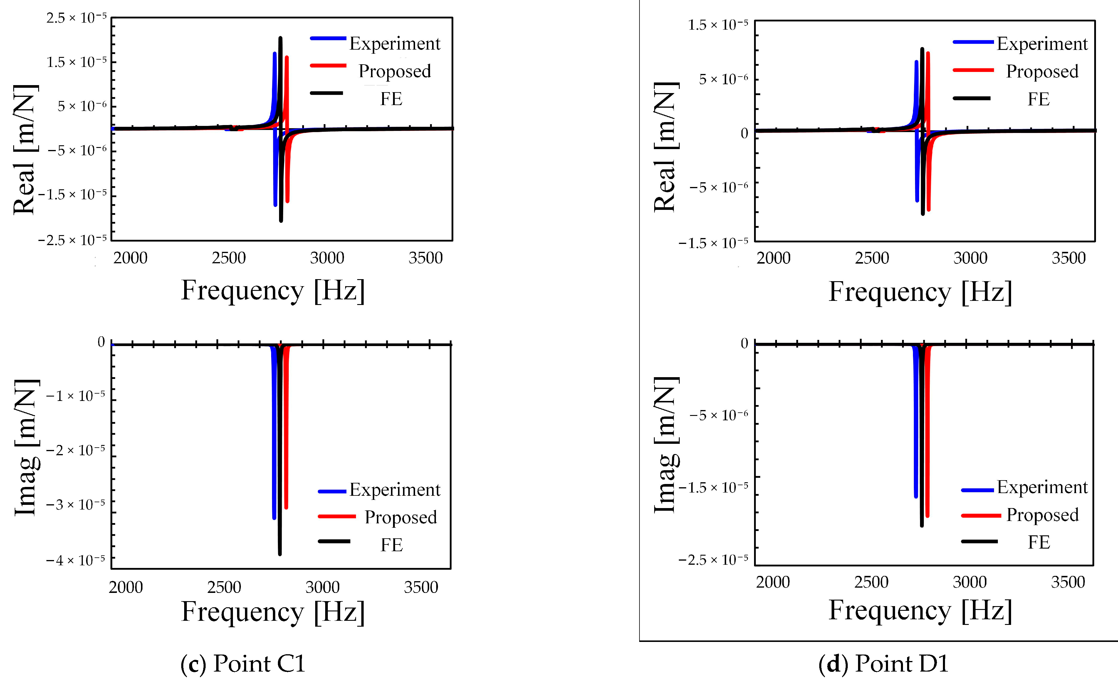
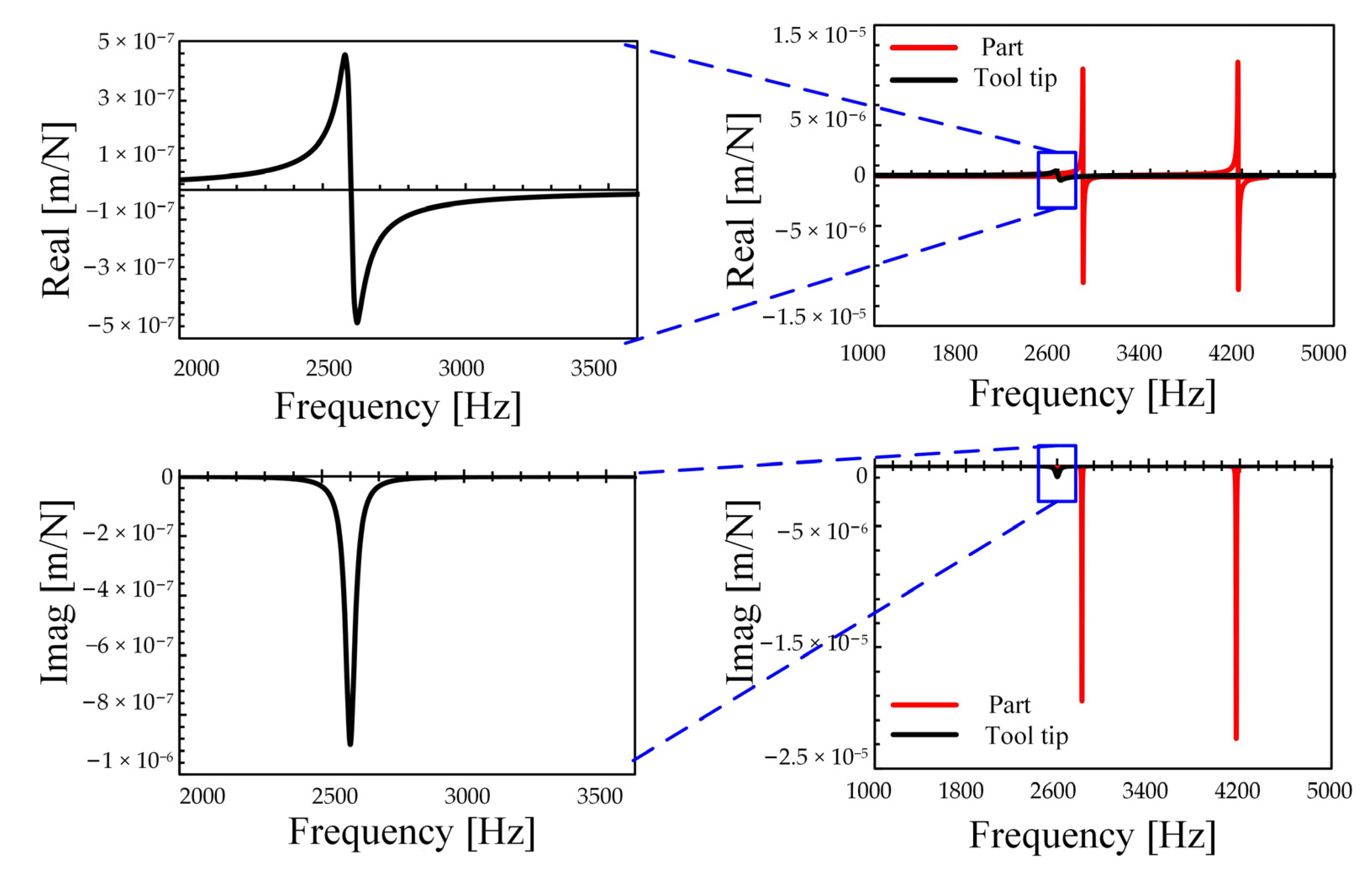
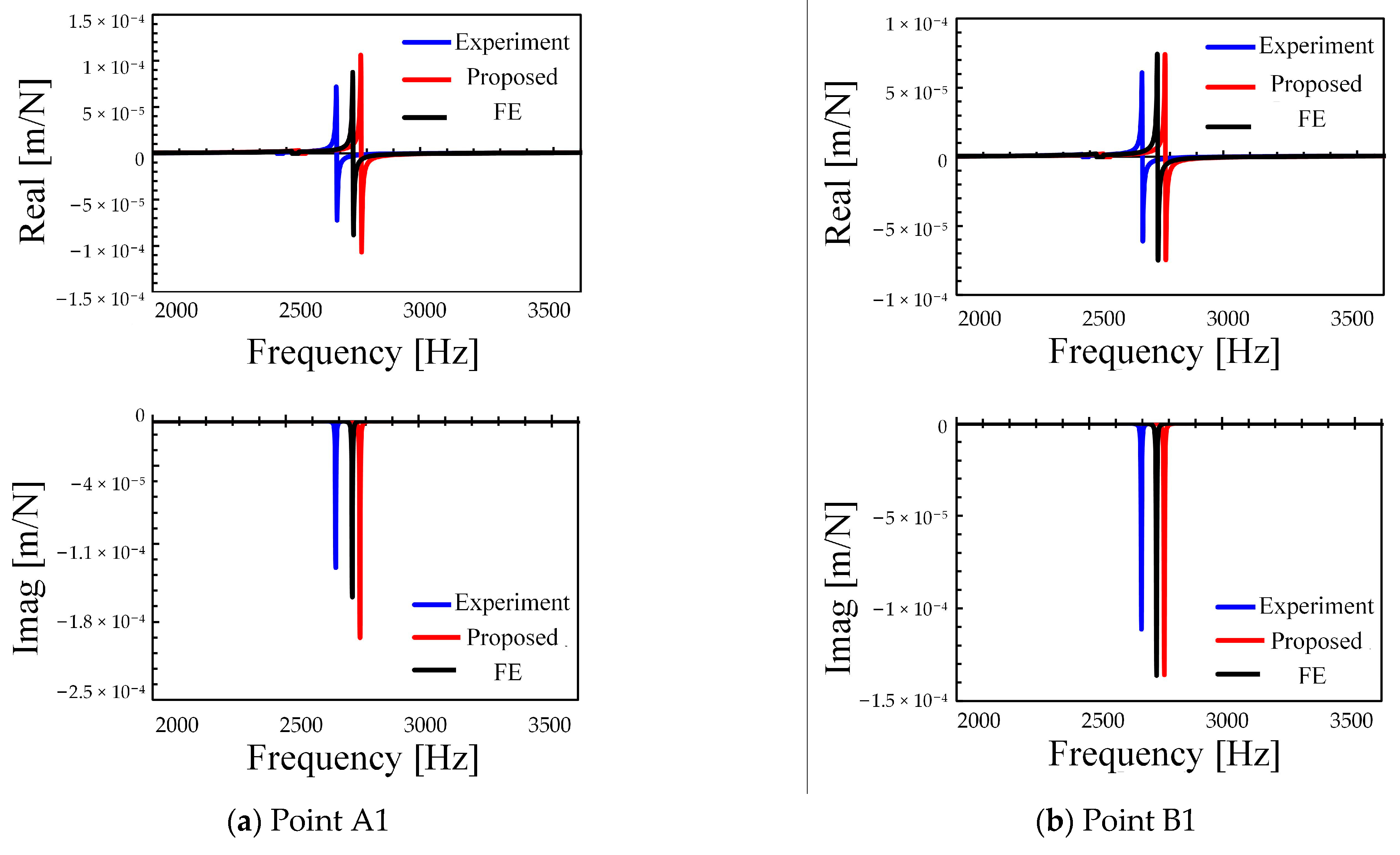
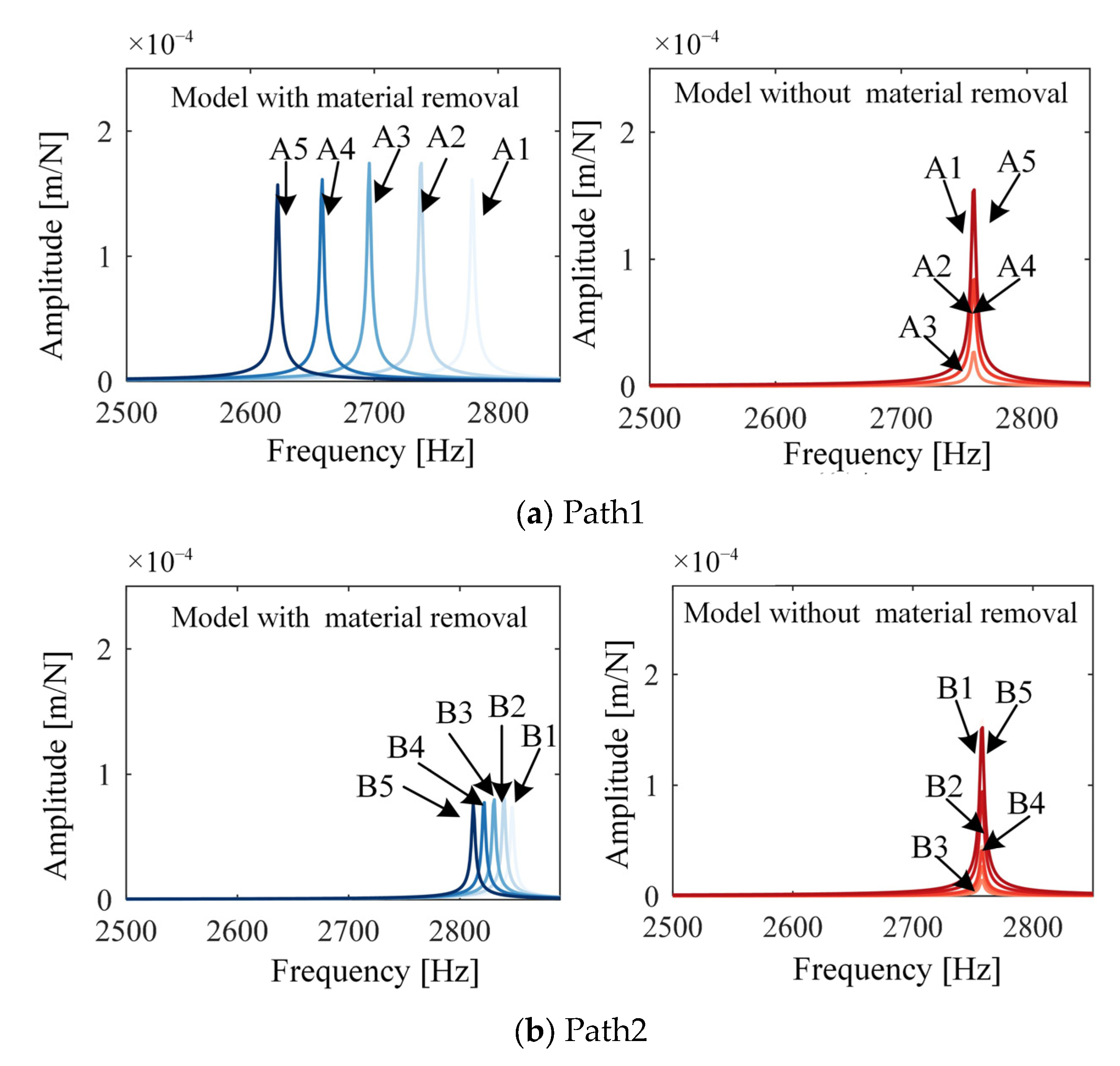
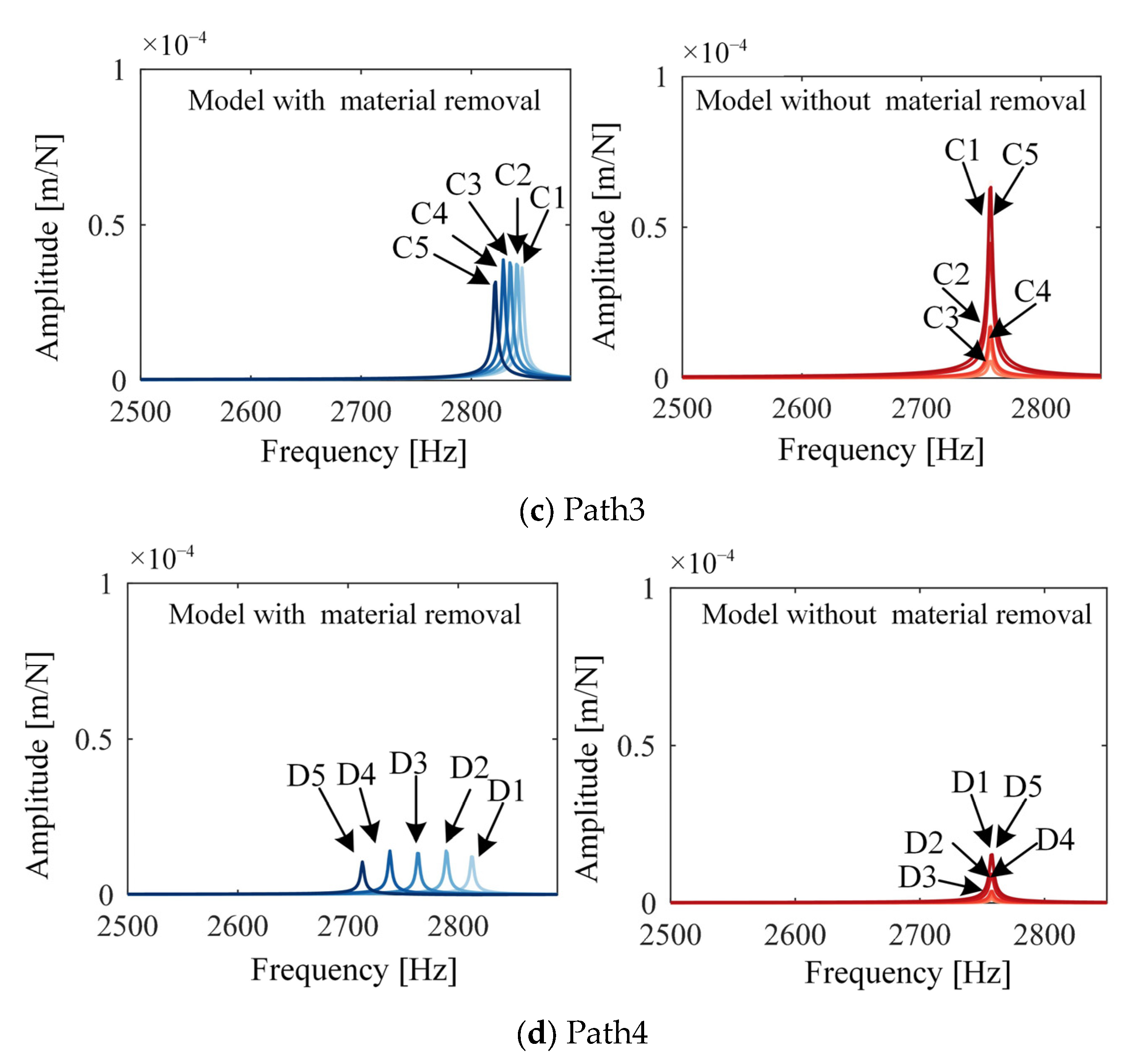
4.2. Verification of Dynamics Model for Thin-Walled Part in Five-Axis Flank Milling

For comparison purposes, the FRFs were also calculated using the finite element (FE) model developed by commercial software Abaqus 6.14 (Dassault Systèmes, Inc., Paris, France) and an eight-node solid brick element was employed to develop the FE model. The exciting force was set to a value of 1 N, and clamping boundary conditions were applied on the base of the benchmark. The element size was assigned as 1 mm. From an investigation of the element size on the FRF prediction results, little influence was found when using even finer elements. The parameters used to predict FRFs, containing material properties, dimensions, boundary conditions, and proportional damping constants, were substituted into the dynamics model. The FRFs were predicted using two methods and the four points A1, B1, C1, and D1 were selected for comparison. Figure 11 shows the experimental and predicted results of the FRF. The comparisons of natural frequency between the dynamics models and the experimental measurements are illustrated in Table 1. The proposed model can reach a similar accuracy to the typical FE model.
The computational efficiency can be reflected from the DOF number of the model. The larger of DOF number, the less efficiency of computation. Comparing with the FE model, a significant reduction in the DOFs can be realized by the proposed model as shown in Table 2. The variation in the part’s geometry during machining is represented by the change in thickness in the corresponding elements for the proposed model, which avoids the updates of the model. The total DOFs in the FE method are almost 8 times those of the proposed model, which proves that the time cost in computation can be reduced significantly by the proposed model.

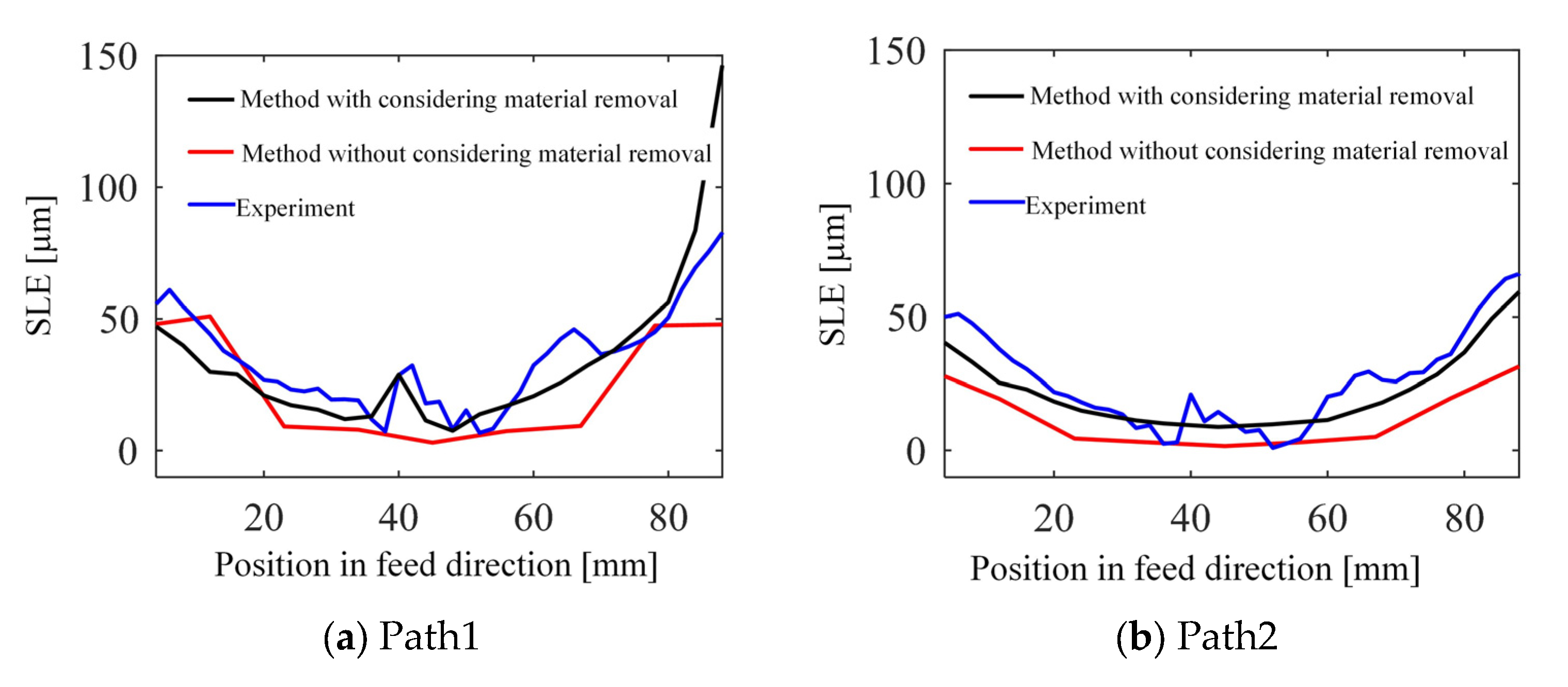
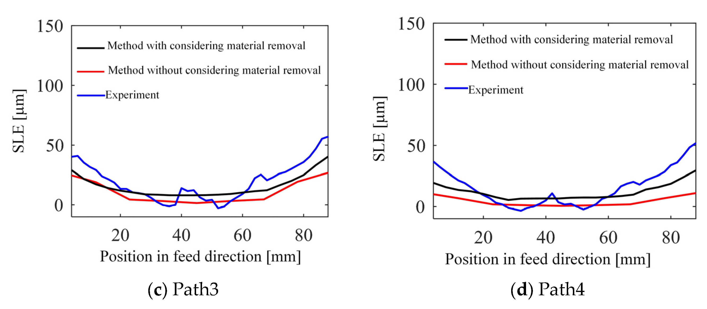
4.3. Verification of Prediction Method for Surface Location Error

In order to make a comparison, the case without varying the dynamics of the part was also performed to predict the FRFs and SLE as well. Both input parameters were the same for these two methods. The points to predict the FRFs in each path are illustrated in Figure 12, and the calculated FRFs are shown in Figure 13. The natural frequency variation in each path was reflected by the model with material removal, and the changing range is illustrated in Table 3. However, the difference in the FRFs of the points in each path is only shown in magnitude for the model without material removal.
Figure 14 plots the SLE obtained by the experiment and the methods with and without considering material removal. It can be seen that the errors in the SLE on the points of each path were all lower for the proposed method, and the average value of SLE errors was reduced from ~10 μm to ~5 μm as illustrated in Table 4. The complex changes in chip thickness at the initial and final positions in the processing direction led to a significant increase in SLE in the corresponding positions.

5. Conclusions

This article presents a computationally efficient and practical method for SLE prediction considering the varying dynamics of thin-walled parts in five-axis flank milling, including a computationally efficient dynamics model and a practical SLE prediction method. The detailed conclusions are summarized as follows:
(1) A new, computationally efficient dynamics model of thin-walled parts considering material removal is developed based on the thin-plate theory and substructure method. The accuracy of the proposed model is verified by the FRF experiments of four points in a thin-walled part during milling, and the errors of natural frequencies are all less than 5%. Meanwhile, the computational efficiency is improved ~8 times by comparing the proposed model with a typical finite element model with a similar accuracy.
(2) A practical SLE prediction method with the consideration of varying dynamics in five-axis flank milling of thin-walled parts is proposed. The coordinate transformation of FRFs and cutting force is realized depending on screw theory and the general cutting dynamics model, which is simple and efficient. The SLE is predicted depending on the forced vibration in five-axis flank milling. A thin-walled part with a sculptured surface is machined and the SLE of four paths is measured to verify the proposed method. It is shown that the average error of the SLE is reduced from ~10 μm to ~5 μm by considering the varying dynamics of the thin-walled part in five-axis flank milling.

Author Contributions

Conceptualization, Y.T. and J.Z.; methodology, Y.T.; validation, Y.T., J.Z. and W.H.; formal analysis, H.L. and W.Z.; writing—original draft preparation, Y.T. and J.Z.; writing—review and editing, Y.T., J.Z. and H.L.; supervision, J.Z. and W.Z.; funding acquisition, J.Z. All authors have read and agreed to the published version of the manuscript.

Funding

This research was financially supported by the National Key R&D Program of China (No. 2018YFB1701901), Shaanxi Science Foundation for Distinguished Young Scholars (2019JC08).

Data Availability Statement

Not available.

Conflicts of Interest

The authors declare no conflict of interest.

References

  1. Quintana, G.; Ciurana, J. Chatter in machining processes: A review. Int. J. Mach. Tools Manuf. 2011, 51, 363–376. [Google Scholar] [CrossRef]
  2. Wang, M.; Yang, C.; Li, Z.; Zhao, S.; Zhang, Y.; Lu, X. Effects of surface roughness on the aerodynamic performance of a high subsonic compressor airfoil at low Reynolds number. Chin. J. Aeronaut. 2021, 34, 71–81. [Google Scholar] [CrossRef]
  3. Morelli, L.; Grossi, N.; Scippa, A.; Campatelli, G. Extended classification of surface errors shapes in peripheral end-milling operations. J. Manuf. Process. 2021, 71, 604–624. [Google Scholar] [CrossRef]
  4. Li, J.; Kilic, Z.M.; Altintas, Y. General Cutting Dynamics Model for Five-Axis Ball-End Milling Operations. J. Manuf. Sci. Eng. 2020, 142, 121003. [Google Scholar] [CrossRef]
  5. Ismail, F.; Ziaei, R. Chatter suppression in five-axis machining of flexible parts. Int. J. Mach. Tools Manuf. 2002, 42, 115–122. [Google Scholar] [CrossRef]
  6. Tsai, J.S.; Liao, C.L. Finite-element modeling of static surface errors in the peripheral milling of thin-walled workpieces. J. Mater. Process. Technol. 1999, 94, 235–246. [Google Scholar] [CrossRef]
  7. Adetoro, O.B.; Sim, W.M.; Wen, P.H. An improved prediction of stability lobes using nonlinear thin wall dynamics. J. Mater. Process. Technol. 2010, 210, 969–979. [Google Scholar] [CrossRef]
  8. Ahmadi, K. Finite strip modeling of the varying dynamics of thin-walled pocket structures during machining. Int. J. Adv. Manuf. Technol. 2017, 89, 2691–2699. [Google Scholar] [CrossRef]
  9. Friswell, M.I.; Garvey, S.D.; Penny, J.E.T. Model reduction using dynamic and iterated IRS techniques—ScienceDirect. J. Sound Vib. 1995, 186, 311–323. [Google Scholar] [CrossRef]
  10. Cunedioğlu, Y.; Muğan, A.; Akçay, H. Frequency domain analysis of model order reduction techniques. Finite Elem. Anal. Des. 2006, 42, 367–403. [Google Scholar] [CrossRef]
  11. Meshreki, M.; Kövecses, J.; Attia, H.; Tounsi, N. Dynamics Modeling and Analysis of Thin-Walled Aerospace Structures for Fixture Design in Multiaxis Milling. J. Manuf. Sci. Eng. 2008, 130, 031011. [Google Scholar] [CrossRef]
  12. Meshreki, M.; Attia, H.; Kövecses, J. A New Analytical Formulation for the Dynamics of Multipocket Thin-Walled Structures Considering the Fixture Constraints. J. Manuf. Sci. Eng. 2011, 133, 021014. [Google Scholar] [CrossRef]
  13. Meshreki, M.; Attia, H.; Kövecses, J. Development of a New Model for the Varying Dynamics of Flexible Pocket-Structures During Machining. J. Manuf. Sci. Eng. 2011, 133, 041002. [Google Scholar] [CrossRef]
  14. Tuysuz, O.; Altintas, Y. Frequency Domain Updating of Thin-Walled Workpiece Dynamics Using Reduced Order Substructuring Method in Machining. J. Manuf. Sci. Eng. 2017, 139, 071013. [Google Scholar] [CrossRef]
  15. Tuysuz, O.; Altintas, Y. Time-Domain Modeling of Varying Dynamic Characteristics in Thin-Wall Machining Using Perturbation and Reduced-Order Substructuring Methods. J. Manuf. Sci. Eng. 2018, 140, 011015. [Google Scholar] [CrossRef]
  16. Ma, J.; Li, Y.; Zhang, D.; Zhao, B.; Wang, G.; Pang, X. Dynamic response prediction model of thin-wall workpiece-fixture system with magnetorheological damping in milling. J. Manuf. Process. 2022, 74, 500–510. [Google Scholar] [CrossRef]
  17. Liu, H.; Xu, X.; Zhang, J.; Liu, Z.; He, Y.; Zhao, W.; Liu, Z. The state of the art for numerical simulations of the effect of the microstructure and its evolution in the metal-cutting processes. Int. J. Mach. Tools Manuf. 2022, 177, 103890. [Google Scholar] [CrossRef]
  18. Kline, W.A.; DeVor, R.E.; Shareef, I.A. The Prediction of Surface Accuracy in End Milling. J. Eng. Ind. 1982, 104, 272–278. [Google Scholar] [CrossRef]
  19. Tlusty, J. Effect of End Milling Deflections on Accuracy. In Handbook of High Speed Machining Technology; King, R.I., Ed.; Chapman and Hall: New York, NY, USA, 1985. [Google Scholar]
  20. Sutherland, J.W.; DeVor, R.E. An Improved Method for Cutting Force and Surface Error Prediction in Flexible End Milling Systems. J. Eng. Ind. 1986, 108, 269–279. [Google Scholar] [CrossRef]
  21. Schmitz, T.L.; Smith, K.S. Machining Dynamics; Springer: Boston, MA, USA, 2009; ISBN 978-0-387-09644-5. [Google Scholar]
  22. Altintas, Y.; Montgomery, D.; Budak, E. Dynamic Peripheral Milling of Flexible Structures: Computer Modeling and Simulation of Manufacturing Processes. J. Manuf. Sci. Eng. 1991, 13, 229. [Google Scholar] [CrossRef]
  23. Budak, E.; Altintas, Y. Modeling and avoidance of static form errors in peripheral milling of plates. Int. J. Mach. Tools Manuf. 1995, 35, 459–476. [Google Scholar] [CrossRef]
  24. Ratchev, S.; Liu, S.; Huang, W.; Becker, A.A. Milling error prediction and compensation in machining of low-rigidity parts. Int. J. Mach. Tools Manuf. 2004, 44, 1629–1641. [Google Scholar] [CrossRef]
  25. Sofuoglu, M.A.; Orak, S. A hybrid decision making approach to prevent chatter vibrations. Appl. Soft Comput. 2015, 37, 180–195. [Google Scholar] [CrossRef]
  26. Li, X.; Guan, C.; Zhao, P. Influences of milling and grinding on machined surface roughness and fatigue behavior of GH4169 superalloy workpieces. Chin. J. Aeronaut. 2018, 31, 1399–1405. [Google Scholar] [CrossRef]
  27. Misaka, T.; Herwan, J.; Ryabov, O.; Kano, S.; Sawada, H.; Kasashima, N.; Furukawa, Y. Prediction of surface roughness in CNC turning by model-assisted response surface method. Precis. Eng. 2020, 62, 196–203. [Google Scholar] [CrossRef]
  28. Ringgaard, K.; Mohammadi, Y.; Merrild, C.; Balling, O.; Ahmadi, K. Optimization of material removal rate in milling of thin-walled structures using penalty cost function. Int. J. Mach. Tools Manuf. 2019, 145, 103430. [Google Scholar] [CrossRef]
  29. Jiao, Z.; Kang, R.; Zhang, J.; Du, D.; Guo, J. Modelling of surface roughness in elliptical vibration cutting of ductile materials. Precis. Eng. 2022, 78, 19–39. [Google Scholar] [CrossRef]
  30. Li, W.; Wang, L.; Yu, G. Force-induced deformation prediction and flexible error compensation strategy in flank milling of thin-walled parts. J. Mater. Process. Technol. 2021, 297, 117258. [Google Scholar] [CrossRef]
  31. Agarwal, A.; Desai, K.A. Tool and Workpiece Deflection Induced Flatness Errors in Milling of Thin-walled Components. Procedia CIRP 2020, 93, 1411–1416. [Google Scholar] [CrossRef]
  32. Li, Z.; Jiang, S.; Sun, Y. Chatter stability and surface location error predictions in milling with mode coupling and process damping. Proc. Inst. Mech. Eng. Part B J. Eng. Manuf. 2017, 233, 095440541770822. [Google Scholar] [CrossRef]
  33. Morelli, L.; Grossi, N.; Campatelli, G.; Scippa, A. Surface location error prediction in 2.5-axis peripheral milling considering tool dynamic stiffness variation. Precis. Eng. 2022, 76, 95–109. [Google Scholar] [CrossRef]
  34. Liu, H.; Birembaux, H.; Ayed, Y.; Rossi, F.; Poulachon, G. Recent Advances on Cryogenic Assistance in Drilling Operation: A Critical Review. J. Manuf. Sci. Eng. 2022, 144, 100801. [Google Scholar] [CrossRef]
  35. Murray, R.M.; Li, Z.; Sastry, S.S. A Mathematical Introduction to Robotic Manipulation; CRC Press: Boca Raton, FL, USA, 1994. [Google Scholar]
  36. Yang, J.; Altintas, Y. Generalized kinematics of five-axis serial machines with non-singular tool path generation. Int. J. Mach. Tools Manuf. 2013, 75, 119–132. [Google Scholar] [CrossRef]
Figure 1. Decomposition of in-process part.
Processes 11 00242 g001
Figure 2. Coupling of substructures.
Processes 11 00242 g002
Figure 3. Five-axis flank machining.
Processes 11 00242 g003
Figure 4. A typical end mill containing helical flutes.
Processes 11 00242 g004
Figure 5. Flowchart for the prediction of SLE.
Processes 11 00242 g005
Figure 6. Machining process of Benchmark.
Processes 11 00242 g006
Figure 7. FRFs testing of tool tip.
Processes 11 00242 g007
Figure 8. Experimental setup and testing points.
Processes 11 00242 g008
Figure 9. FRFs’ comparison between part and tool tip.
Processes 11 00242 g009
Figure 10. Measurement of surface location error of part.
Processes 11 00242 g010
Figure 11. FRFs’ comparison between experiment and prediction.
Processes 11 00242 g011aProcesses 11 00242 g011b
Figure 12. FRF prediction points in each path.
Processes 11 00242 g012
Figure 13. FRF comparison between two models.
Processes 11 00242 g013aProcesses 11 00242 g013b
Figure 14. Surface location error comparison between measurement and proposed and compared methods.
Processes 11 00242 g014aProcesses 11 00242 g014b
Table 1. Natural frequency comparison between experiment and prediction.
PointExperiment [Hz]Proposed Method [Hz]Error [%]FE Method [Hz]Error [%]
1268727793.4227492.31
2269627823.1627532.11
3276828492.9127950.98
4276228171.9727901.01
Table 2. DOFs’ comparison of two models.
PointFE Method (ABAQUS)Proposed Method
193,32413,332
290,29413,332
387,29613,332
484,23413,332
Table 3. Natural frequency variation of part during milling.
PathMinimum [Hz]Maximum [Hz]Varying Ratio [%]
1261227796.39
2278228472.34
3281128491.35
4271328173.83
Table 4. SLE comparison.
PathExperiment
Value [μm]
Method with Considering Material RemovalMethod without Considering Material Removal
Value [μm]Error [μm]Value [μm]Error [μm]
135.3934.241.1525.589.81
226.5821.764.8213.3113.27
320.1115.464.6512.167.95
415.5311.873.664.7610.77
Disclaimer/Publisher’s Note: The statements, opinions and data contained in all publications are solely those of the individual author(s) and contributor(s) and not of MDPI and/or the editor(s). MDPI and/or the editor(s) disclaim responsibility for any injury to people or property resulting from any ideas, methods, instructions or products referred to in the content.

