1. Introduction
Liquefied natural gas (LNG), which can be considered pure methane at cryogenic temperatures, is gaining increasing interest as an energy vector. Indeed, it allows for a greater plurality of providers, reducing the risks of supply discontinuity. In this regard, even if the vast majority of global LNG exports comes from a few major countries, smaller producers are also increasingly interconnected with other countries. The new scenario amplifies the chances of the formation of new trade routes [
1]. The availability of liquefied natural gas in the world is wide and is expected to expand in the coming years, owing to unconventional fossil production sources, such as shale gas or synthetic from coal gasification/methanation but also renewable ones, such as biomethane, which may be the best choice for the conversion of biomass into biofuels [
2]. For these reasons, the current global LNG trade volume meets 12% of the gas demand and will continue to increase in the future, reaching up to 22% of the natural gas consumption [
3].
LNG technologies have long been used but only recently found widespread employment on medium and small scales compared to the traditional cycle of liquefaction, transport by ship, regasification and injection into the gas network. The small-scale LNG market includes both the production of LNG in small plants [
4] and the various direct uses as a fuel. In this emerging market, the volumes of LNG and the related infrastructures are expected to grow [
5], although relatively less compared to the total amount of imported LNG. Indeed, LNG logistics provide for displacing fuel with tankers and its storage in special deposits. Therefore, LNG is available for many uses, such as land, railroad, ship, air, agricultural and earthmoving machinery. It is also suitable for supplying distribution networks and industries far from gas networks; today often operating with propane or diesel fuel. In particular, LNG is appropriate for cold ironing in ports, which will be mandatory in the coming years [
6]. Moreover, direct use is favored by the distributed production of cryogenic fuel through upgrading and liquefaction of biogas from organic feedstock. This implies advantages on CO
2 emissions compared to diesel, considering the whole life cycle analysis [
7]. Even greater benefits can be obtained on storage since 1 m
3 of LNG corresponds to approximately 2 m
3 of compressed natural gas in cylinders at 200 bar and 600 m
3 at atmospheric pressure.
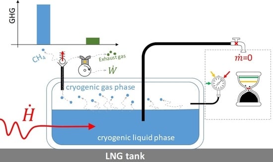
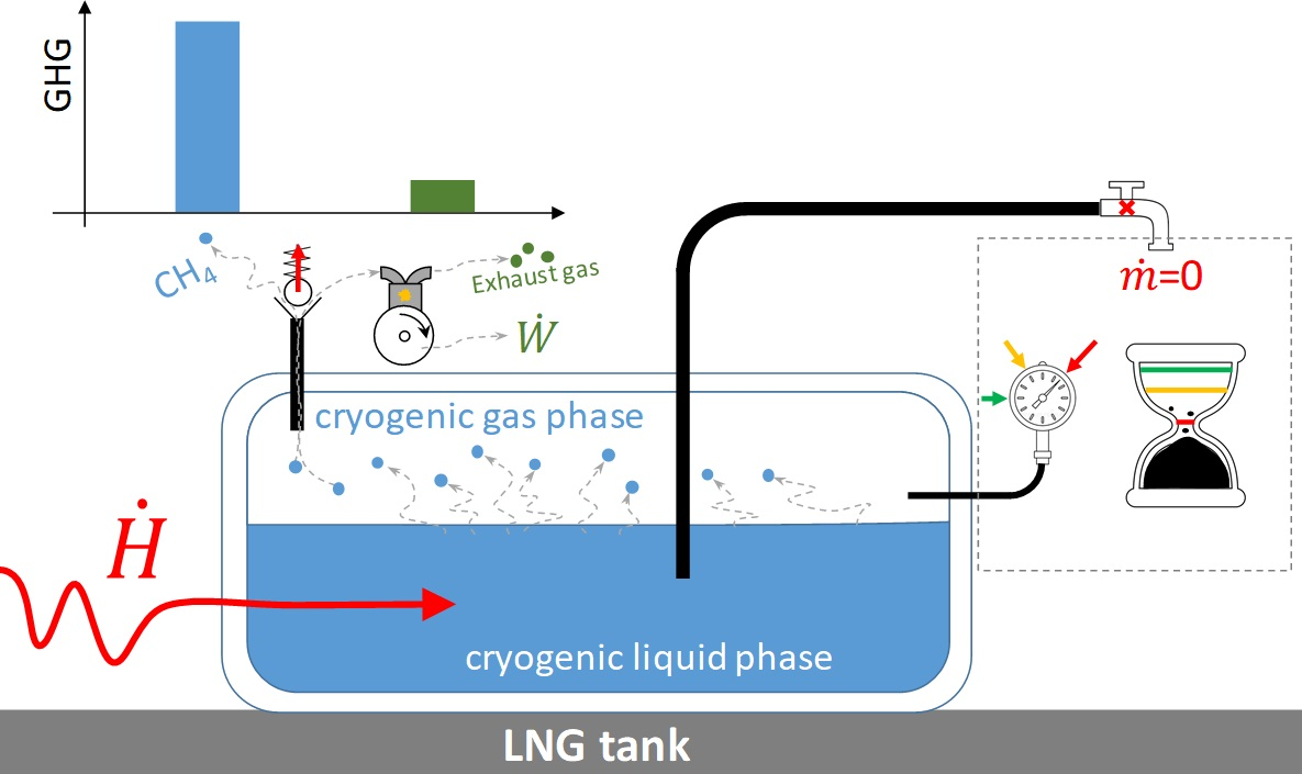
In the case of ship transport and liquefaction and regasification terminals, fields with a capacity of millions of cubic meters of LNG are required. Instead, in small-scale cases, there are tanks that can be considerably smaller. However, in all cases, there is the problem of containing greenhouse gas emissions related to the boil-off gas (BOG) released. This eventuality arises mainly in the event of prolonged absence of drawing of liquid from the tank, but also during the tank loading and unloading processes. The normal operating conditions of cryogenic tanks foresee a slight increase in pressure compared to the nominal value. Exceeding this threshold can damage the tank and is, therefore, dangerous. For this reason, the tanks are equipped with a vent valve of the evaporated fraction. The system is calibrated to open automatically at a certain pressure value to release the excess gas to the outside, until the normal operating pressure values are restored.
Generally, the BOG problem is irrelevant in production and regasification terminals, where it is possible to predict the boil-off rate (BOR) with high precision and to implement containment strategies [
8]. The authors of [
9] evaluated the annual flow of attainable excess LNG recovering the generated BOG from an LNG export terminal with a capacity of almost 16 million standard cubic meter. They found that a greater profit is associated with LNG sub-cooling to reduce BOR, than with BOG processing for re-liquefaction. In [
10], a comparison of two different BOG re-condensation systems with a BOG use in a combined gas turbine fueled with both LNG and BOG is proposed. The solution of using BOG for energetic purposes is the most convenient, even if only when the electricity price is high, due to the complexity of the exploitation plant. Similar results are reported in [
11], where a combined cycle plant of 100–300 MW is considered to use the BOG of the regasification terminals. The authors of [
12] considered LNG regasification terminals with tank sizes from 100,000 to 400,000 m
3 and an LNG recirculation line used for cooling cryogenic pipes. The study results show that adopting a minimum recirculation rate is the best operating policy for BOR reduction in receiving terminals.
Solutions similar to those for the terminals are also adopted for use on transport ships, such as re-liquefaction [
13,
14], with others aimed at the energy exploitation of BOGs. Applications can be found in dual fuel diesel-gas propulsion engines or on-board supply of auxiliary motors. Kim et al. considered the case of BOG as extra fuel for generator engines in LNG-fueled vessels with a cargo capacity of 5000 m
3 [
15]. BOG is used to charge a battery energy storage system. Adding the contribution of CO
2, CH
4, and N
2O, the results highlight a greenhouse gas (GHG) reduction from 5% to 17% in respect of the simple BOG combustion. Kalikatzarakis et al. focused on the conditions of an LNG-fueled oceangoing ship for typical long and short voyages [
16]. They found a BOG compression capacity of 450 kg/h effective for avoiding the tank overpressure, with three or four activations for voyage. In [
17], a strategy for using the cryogenic temperature of the BOG is analyzed by making air flow inside the insulation space of a 40,447 m
3 LNG tank for a typical membrane module of LNG transport ships. The results show that the system can minimize BOG formation, thus, reducing the need for re-liquefying.
Small-scale direct uses of LNG are pushing the spread of cryogenic tanks of reduced capacity that fall within the range of hundreds to thousands of liters. Systems that use these small tanks are unlikely to have economies that can justify expensive methods for the exploitation of BOG. In addition, there can be layout problems due to the space and additional weight required for the installation of such plants. Therefore, the logistics of the distribution-consumption of the fuel is fundamental in order to reduce the transfers and downtime of the plants to limit the formation of BOG. Therefore, if necessary, BOG is expelled directly into the atmosphere or after being oxidized by catalytic burners or torches. Direct ejection into the atmosphere entails considerable problems of CO
2 equivalent emissions (CO
2,EQ). Indeed, CH
4 has a 100-year global warming potential (GWP) equal to about 30 times (about 27 if it is coming from non-fossil sources) that of CO
2 [
18]. Additionally, there are safety issues. Barelli et al. analyzed a 450-liter LNG tank installed on a truck [
19]. The results show that measured BOR spikes were greater than those expected; for example, suggesting the installation of ventilation systems to lower the flammable gas concentration and mitigate the explosion risk in closed environments. Although different applications are possible for BOG recovery from small capacity tanks, such as external BOG storage, energy conversion or on-tank systems to re-liquefy or convert BOG (for heating or battery charging), there are no dedicated studies in the literature. This study aims to reduce this gap by analyzing the BOG problem for a small tank of the type used on trucks or buses. A 500-liter tank was considered for which the daily BOR was estimated. For the recovery of the BOG, the possibility of adopting a generator that can be easily installed on-board on heavy vehicles, such as trains, tankers, but also fixed tanks, were considered. It allows the conversion of BOG into energy to be used, for example, to recharge batteries. Based on the estimated BOR, a 2-stroke engine of very small weight and size with a power of 1 kW was selected. A numerical model was calibrated with experimental data obtained with gasoline fueling and used to dimension the gas supply system. Finally, the performance of the gas prototype was measured on a test bench and compared with other strategies. If the right engine technologies are adopted, the results of the study highlight the convenience of using the BOG energy conversion system, with a reduction in GHG emissions, even with respect to the burning of BOG before being released into the atmosphere.
2. Materials and Methods
This work studies the feasibility of using small internal combustion engines for BOG energy exploitation. First, the maximum BOR from a small LNG tank was estimated. Then, a 2-stroke gasoline engine was adapted to run on gas using numerical and experimental tools.
2.1. Evaluation of the Maximum BOR and Sizing of the Internal Combustion Engine
The operating pressure of small LNG tanks, commonly used in heavy transport, is around 11 bar immediately after refueling. The corresponding storage temperature of the liquid and vapor phases in equilibrium (saturated LNG) is about −120 °C (153 K). However, the pressure in the tank can increase over time. Therefore, two threshold pressures are set for opening and closing a vent valve.
Table 1 shows some properties of LNG (considered composed of 100% CH
4) in the different operating conditions of the tank. The values were calculated using tables for the thermophysical properties of methane.
The BOG relief valve opens when the saturation pressure exceeds the maximum threshold (
O) and closes when it falls below the set level (
C). In the tank, once part of the vapor phase is expelled to reduce the pressure, part of the liquid phase evaporates and low temperature until a new equilibrium is generated between the two phases. The ejection of BOG mainly occurs when the system fed with LNG is on pause, without liquid or vapor phase consumption. Indeed, fuel consumption causes an imbalance between the phases and the subtraction of heat from the tank, keeping the LNG at a low temperature. The unitary heat exchange coefficient of these tanks is too low to guarantee a residence time of at least 4–5 days without the ejection of BOG in the absence of fuel requests by the utilities. Once the holding time has elapsed, if no consumption from the users continues, the maximum BOR achieves. It is possible to proceed in a simplified way to estimate the maximum BOR. The 500-liter tank could be approximated as a cylinder with a diameter of 0.50 m and a length of 2.55 m. An exchange surface
A of almost 4.5 m
2 is thus obtained. The heat input entering the tank can be evaluated by Equation (1), assuming the heat transfer coefficient
k is equal to 0.02 W/m
2K, the ambient temperature
is equal to 298 K and the temperature inside the tank
is equal to approximately 159 K (averaged between the thermodynamic conditions
O and
C).
Supposing that the liquid phase initially occupies 80% by volume (
V) of the tank, the mass (
) is given by Equation (2), where
V is in m
3 and
is the density of the liquid in the thermodynamic state
C.
Simplifying the phenomenon, due to the heat introduced into the tank, part of the liquid will evaporate, and the equilibrium conditions move to gradually higher saturation pressures, with a consequent increase in temperature, until the pressure reaches the threshold of the open relief valve. The energy absorbed by each unit mass of liquid in the passage from the thermodynamic state
C to that
O is the difference between the enthalpies associated with the liquid in the two states, approximately 10 kJ/kg. Therefore, the total amount of heat
Q that must enter the tank to change from the thermodynamic state
C to
O is approximately 1350 kJ. This energy passes through the cylinder walls with the power derived from Equation (1). Therefore, the time required from
C to
O can be calculated by Equation (3).
To compensate for the amount of heat absorbed by the liquid, a certain amount of BOG is expelled from the tank. Assuming for the latent heat of vaporization of LNG (
) is equal to the enthalpy difference between the liquid and gaseous phases, the average value between the two states
O and
C, it is possible to calculate the quantity of BOG to be removed (
) to restore the liquid in state
C with Equation (4).
From Equations (3) and (4) it is possible to evaluate the BOR necessary to keep the tank in safety conditions at approximately 120 g/h (0.09% of the initial LNG mass per day), in the absence of consumption. This value, obtained in a simplified way, is similar to others available in the literature. In [
19], a BOR of 80 g/h (0.11% of the initial mass of LNG per day) is reported for a 450-liter tank at 15.8 bar of maximum pressure. In [
20], a BOR of 0.11% was calculated for LNG cargoes of 35,000-m
3 at a maximum pressure of 1 bar. Instead, in [
21] the BOR was evaluated considering the distribution of the heat into the vapor and liquid. The effect of change in the liquid level, for a 260,000-m
3 LNG storage tank at 1 bar maximum pressure, results in 0.01% to 0.12%, respectively, for an 80%- and 10%-filled tank.
The estimated BOR corresponds to a thermal input of about 1.7 kW suitable for continuously powering an engine of about 400 W (with an overall efficiency of about 25%). Therefore, an engine with higher maximum power, in the 1−1.5 kW range, can be used to consume the maximum BOR by running at regular intervals, with an overall workload of about 5−10 h per day.
2.2. Method for Fueling a Small Engine with BOG
The ejection of the BOG occurs intermittently, with high flow rate peaks at the overpressure corresponding to the opening conditions of the relief valve. Therefore, the BOG should be stored in a small cylinder to be used gradually at a slightly lower pressure than the LNG tank. Alternatively, the BOG could be withdrawn from the tank at pre-set intervals, with a flow rate higher than the maximum BOR, keeping the tank at a pressure lower than that which generates the opening of the safety valve without the need for cylinder accumulation. In any case, the BOG outlet pressure is too high to directly feed an engine, either with a mixer or a timed injection system. It is necessary to condition the BOG to send it to the fuel system and dose it appropriately. The fuel system must allow the correct pressure for the fuel injection with the air sucked in by the engine. The fuel pressure should be 1 bar for the system with the Venturi mixer and about 3−5 bar for the injection system. Therefore, the fuel conditioning system must have a suitable pressure regulator plus an electronic control unit in the case of timed injection. The timed injection system adds the fuel using the injector-opening times mapped in the control unit. The mixer system can be mechanical or include electronic flow control to improve accuracy. Like a carburetor, the airflow in a mixer throat sucks a proportional quantity of fuel through a series of holes. Furthermore, in the case of a 2-stroke engine, it is necessary to adopt a system for adding the lubricating oil, which cannot be mixed with the fuel as is the case for small gasoline engines.
Due to the low target power, for the experimental activity, a small gasoline 2-stroke engine with carburetor supply and crankcase compression was selected, of the type used for hand tools. The engine has a 42 mm bore and a 43-cm
3 displacement. This choice was made to test the less energetically efficient system but the cheapest one, with a better weight/power ratio, compactness, constructive simplicity, handling, and maintenance costs.
Figure 1a shows the engine with the BOG fuel and lube oil management systems.
Figure 1b shows the effect of oil on the indicated mean effective pressure (IMEP) of the engine at 7000 rpm with a constant fuel supply. The oil droplet injection frequency was set to the minimum value (0.5−0.7 Hz, equivalent to about 5−10 g/h) that caused a slight increase in IMEP. This indicates that the oil reaches the combustion chamber lubricating all the engine parts.
2.3. Experimental Setup for Performance Measurements
The engine was equipped with two pressure transducers to measure the pressure cycle, one in the crankcase and the other in the combustion chamber, and a magnetic angular encoder on the shaft to associate each pressure value with the corresponding angular position of the crankshaft. The engine was installed on a test bed coupled with an electric motor driven by an inverter. The fuel used in the experimental tests for simulating the BOG is natural gas in cylinders with a high concentration of CH
4. The exhaust gas analyses and air/fuel measurement were performed with the equipment in
Table 2. When unburned hydrocarbon (UHC) emissions were over the instrument range, the exhaust gas was diluted before analysis. Each test point was repeated thrice, resulting in more data scatter than instrumentation imprecision due to the effect that little variations in test conditions have on performance. On average, the standard variation was 3–5% for measured parameters such as consumption and 5–10% for calculated parameters such as efficiency.
2.4. Numerical Modeling of the Engine
A one-dimensional (1D) numerical model of the engine was created with the software GT-POWER. The model allows to define the characteristics of the BOG fuel system and evaluate the engine performance, with the variation of some parameters that cannot be controlled in the experimental tests. The software decomposes each element (duct/volume) discretely into a certain number of sub-volumes of reduced dimensions within which it considers the scalar properties of the fluid constant (mass, pressure, temperature, internal energy, etc.). Then, it calculates iteratively until the convergence of the properties of the individual volumes through mass and energy balance equations. Modeling requires defining geometric properties and boundary conditions (such as wall heat transfer coefficients) and setting up sub-models for more complex phases (such as combustion or scavenging). The engine was simulated with two variable volumes: crankcase with a compression ratio of about 1.5 and cylinder with a compression ratio of about 10. They are in communication with each other and with the intake and exhaust ducts via ports, whose sections are variable with the crank angle. To simulate the input fuel into the intake duct through a carburetor or mixer, an injector with a fuel flow rate (
) regulated according to Equation (5) was implemented.
where:
is the discharge coefficient of the jet;
is the diameter of the fuel jet different from gasoline and BOG;
is the difference between the ambient/room pressure and the pressure into the Venturi’s throat;
is the fuel density;
is a calibration constant experimentally obtained for the gasoline case.
In this way, the fuel adduction is not continuous but occurs when the depression in the Venturi’s throat is sufficient to suck in the fuel, as in the test condition. The model is valid for gasoline and BOG supply, which is the diaphragm of the last stage of the reducer subject to ambient pressure as in the gasoline case. A throttle valve was also added for load regulation but set to maximum opening conditions to simulate the engine at full admission.
The combustion is simulated by implementing a Wiebe model [
22], experimentally calibrated with the pressure cycles acquired with gasoline fueling. Instead, to evaluate the heat exchange inside the cylinder and crankcase, the implemented model is based on the Woschni correlation [
23]. The scavenging phase involves another sub-model. During scavenging, a certain fraction of the intake mixture short-circuits toward the exhaust without taking part in the combustion The comparison between UHC experimentally measured and predicted by the model was used to calibrate the scavenging. This approach is sufficiently approximate because the UHC from partial combustion of the fuel trapped in the cylinder is significantly lower than UHC from scavenging.
Figure 2 shows the schematic of the 1D model.
3. Results and Discussion
The small-engine model was initially calibrated with experimental data obtained with gasoline operation. Subsequently, the model was adapted to work with the BOG and used to define the most appropriate size of the outflow section of the mixer to run with regular time intervals and the maximum-expected BOR. Then, the BOG fueling was experimentally implemented on the engine and its performance was measured. Finally, the CO2,EQ, evaluated for the experimental prototype and more complex engines, was compared with that corresponding to the emission of BOG in the atmosphere directly or after burning.
3.1. Calibration of the Gasoline Model with Experimental Data
The calibration of the model made it possible to describe, with a good approximation, the operation of the gasoline engine. To evaluate the goodness of the results obtained from the simulation, comparisons were made between the predicted results and the experimental results of the main operating parameters of the engine.
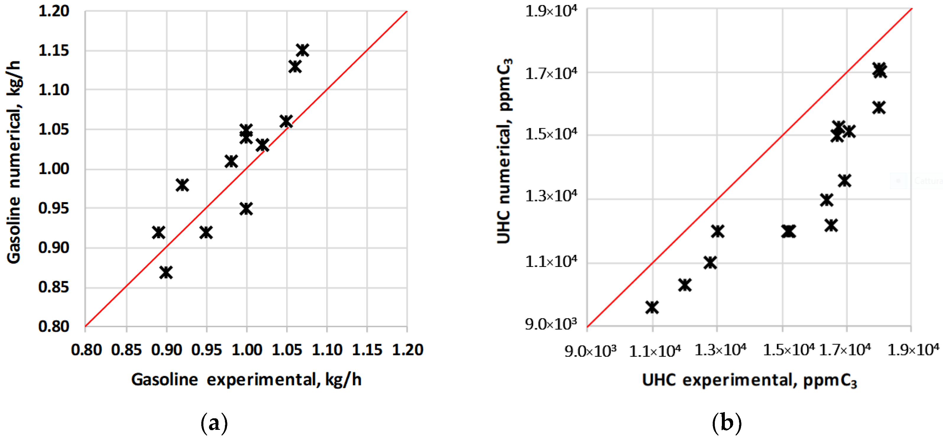
Figure 3 shows, for example, the comparison of the fuel consumption and UHC flow rate at the exhaust evaluated at different engine speeds at maximum admission. Comparisons between experimental results and forecasts are very reliable, particularly for mass flow rates closely linked to the 1D quantities. The observed trend of UHC emissions is correctly simulated, even if the absolute values are slightly underestimated. Since the trend strongly depends on the sub-models used, in particular scavenging, a compromise was made in the choice of calibration parameters due to the interaction between each sub-model.
Figure 4 shows the predicted versus observed pressure cycles at the minimum and maximum engine speed both in the cylinder and crankcase.
The congruence between the curves in the cylinder is an index of proper modeling and calibration of the heat exchanges and the combustion model. The crankcase pressure cycle is well simulated except for the peak, slightly underestimated by about 0.4 bar for the cases reported. This peak is due to the compression effect of the burned gases in the cylinder on the fresh charge in the carter when the transfer ports are opened. However, since the fluid dynamic of the engine is considerably complex compared to simple 1D modeling and since this pressure difference does not have a significant impact on engine performance, the approximation of the model was accepted.
3.2. Numerical Design of the Engine with the BOG Supply
Some modifications have been made to the model to predict the performance of the BOG-fueled engine. The properties of the fuel fed into the intake manifold and the diameter of the passage hole have been changed. The section was chosen to obtain a BOG flow rate in a stoichiometric concentration with the intake air. This choice significantly differentiates the BOG from the gasoline base case. Indeed, the air/gasoline mixture of the original engine must be very rich for engine-operating stability. In contrast, stoichiometric fueling allowed by BOG permits to reduce fuel consumption and UHC exhaust emissions. This choice is possible because the BOG, being gaseous, mixes quicker than gasoline with the air, eliminating the need for enrichment. Regarding the combustion, since a calibration of the Wiebe model for operation at BOG is not available, two simulations were carried out. In one (indicated with fast), the combustion phase was set identically to the gasoline case as the BOG did not influence the combustion speed. In the other (indicated with slow), slower combustion was assumed for the BOG, with an average speed reduced by about 30%, acting on the parameters of the Wiebe model. Experimental data show that the turbulent flame propagation speed was reduced when switching from gasoline to methane fuel [
24]. From an operational perspective, it would be possible to anticipate the spark time, in the case of BOG compared to gasoline, to phase correctly the slower combustion with the crank angle.
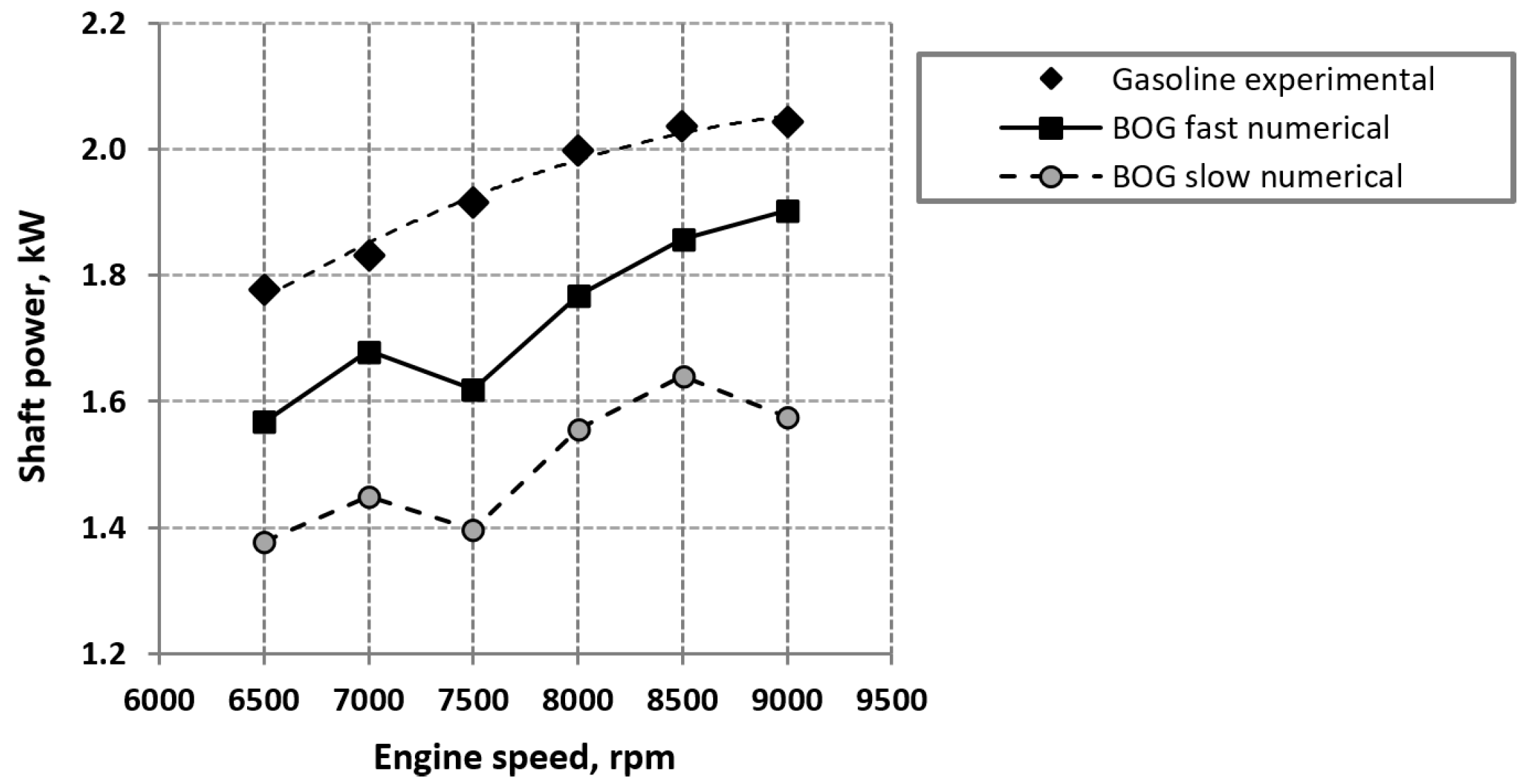
From the simulated results, a reduction of the maximum shaft power at all engine speeds was found,
Figure 5. The results are associated with a lower air mass flow rate compared to gasoline due to the space occupied in the manifold by the gaseous fuel.
The simulations with faster combustion, approximating the setting of higher ignition advance for BOG than gasoline, provide more power due to the better combustion positioning to the crank angle; thus, also resulting in higher overall engine efficiency and lower emissions. Despite the lower power delivered compared to gasoline, the fuel system is oversized for the maximum BOR. Therefore, a 30% reduction in the diameter of the throat section of the mixer was determined using the model. The solution decreases the maximum air flow rate and allows to achieve a power supply in the range of 1−1.5 kW. The fuel feed hole was also reduced to maintain mixture conditions close to stoichiometric.
3.3. Experimental Performance of the BOG Prototype
As suggested by the simulation results, the engine was modified, substituting the carburetor with the defined mixer for the BOG supply. The ignition advance was the same as in gasoline because it cannot be easily changed, as it depends on some mechanical components and construction features.
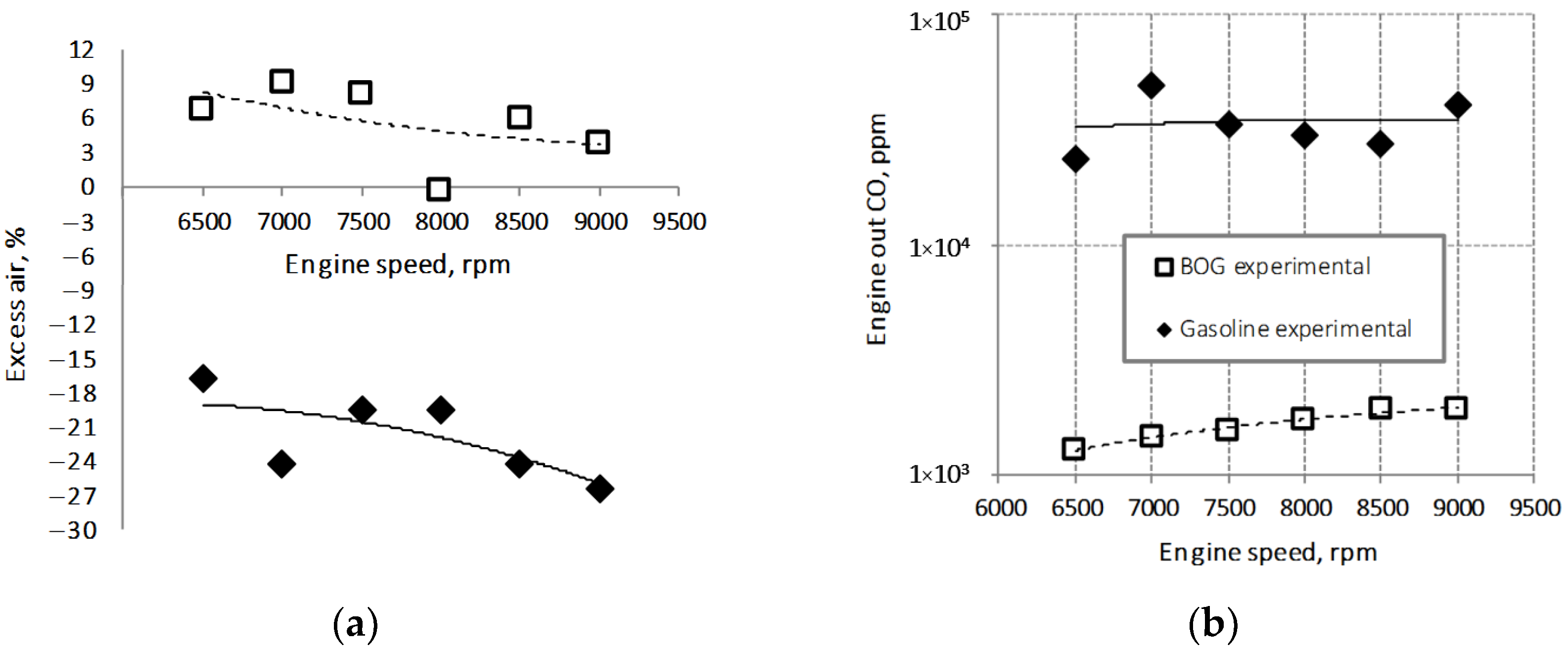
Figure 6 shows the experimental comparison of BOG with gasoline fueling through the curves of excess air and CO emissions. The excess air results in oxygen that is not consumed during combustion, if positive, and in partial fuel burning with high CO and UHC emissions, if negative.
The BOG feed resulted in the stoichiometric-lean mixtures range, in line with what was foreseen in the modeling phase, with advantages compared to the gasoline case of a considerably rich mixture,
Figure 6a. With stoichiometric-lean fueling, it is possible to minimize the fuel in the exhaust caused by the short circuit during scavenging and due to partial combustion. Therefore, CO emissions are significantly reduced with respect to gasoline, more than one order of magnitude, thanks mainly to the excess air,
Figure 6b.
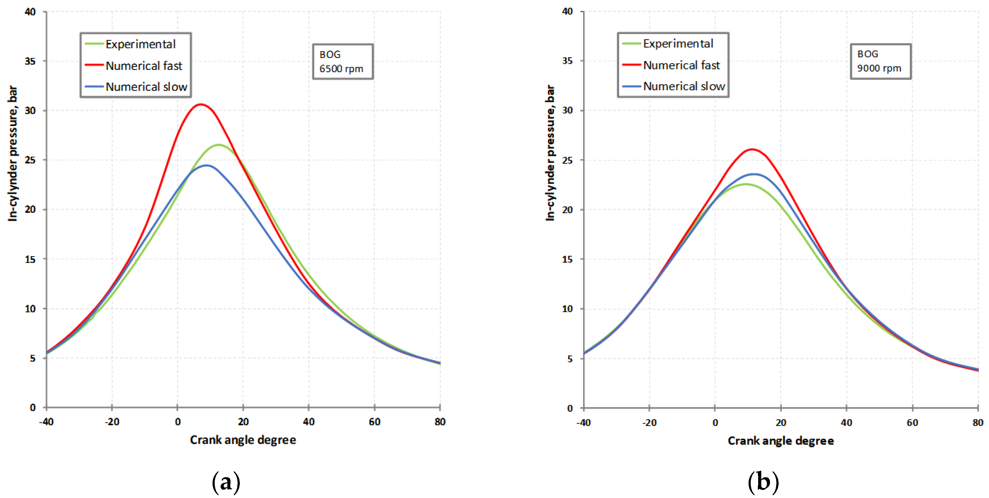
To assess the best performance of the BOG engine with the observed data, the numerically evaluated case with fast combustion, indicative of an increase in the combustion advance, was considered. Therefore, the experimental case was compared with the model predictions.
Figure 7 shows in-cylinder pressure at the minimum and maximum engine speeds. The slow combustion simulation better approximates the observed cycle according to the fact that the flame velocity of methane is lower than that of gasoline, while the spark advance for BOG was the same as for gasoline.
An increase in the ignition advance would allow obtaining a combustion development closer to the top dead center of the cylinder, with higher pressure peaks more similar to those simulated with the faster combustion.
As with pressure cycles, the slow combustion cases also better approximate the power measured (
Figure 8a). A correct combustion timing would allow for greater operating efficiency (
Figure 8b) since anticipating combustion with respect to the opening of the exhaust port, the heat expelled with the exhaust gases is significantly reduced by about 13% according to the 1D model. It is precisely the greater overall efficiency that increases in the power supplied.
Figure 9a shows the fuel mass flow rates, which are in close agreement with the experimental data and little affected by the set combustion mode. In contrast, the combustion mode, and therefore, a correct ignition advance in practice, significantly influences the overall percentage of fuel present in the exhaust,
Figure 9b. The right combustion timing leads to more complete combustion, reducing the UHC from an average value of 18% (slow numerical case) to 16% (fast numerical case). As in the case of gasoline, the model shows an underestimation of UHC, mainly due to the scavenging sub-model.
3.4. Performance Comparison Expected from Different BOG Management Strategies
For a comparison of different BOG control strategies from a cryogenic tank, the experimental data obtained from a 2-stroke engine are considered. The performance was evaluated by the model in the case of optimized ignition advance. Two more cases of more complex engines will also be considered: (i) a 2-stroke engine with timed injection at the transfer ports; (ii) a 4-stroke engine. The first solution would lead to a slight reduction in the UHC short-circuited to the drain, assumed to be less than 20% compared to the case with an experimentally studied mixer. The UHC reduction is not very high since, even with timed injection, the fuel is still injected with the exhaust port always open. As a result, the increase in overall conversion efficiency will also be little. The use of the 4-stroke engine results in a considerable reduction in the UHC, as there is no scavenging phase. The UHC will be even lower if a timed injection system is used. Therefore, an increase in efficiency compared to the case of the 2-stroke was assumed. Moreover, the combustion efficiency could also be slightly higher, as the 4-stroke has a longer expansion phase than the 2-stroke and, therefore, more time for any post-combustion phenomena.
The GWP derived from the direct emission of BOG into the air with the possibility of exploiting the mechanical and thermal energy produced by the selected engines was compared. Finally, to save the estimation of LNG due to the use of the BOG energy, some prudential reference values have been assumed for the conversion efficiency into thermal and electrical energy calculation. Therefore, the LNG savings were associated with an avoided CO
2 production.
Table 3 shows the values of the constants used for the comparison.
The performances, in terms of CO
2,EQ production per gram of BOG, shown in
Table 4 were determined as follows. The corresponding GWP was associated with each unit of BOG issued. If introduced as it is into the atmosphere, the GWP of the BOG must be considered. This corresponds to that of CH
4, equal to 29.8 on a 100-year basis. If the BOG is burned before emission, the CO
2 produced must be considered equal to 2.74 g for each gram of BOG. Finally, different contributions must be considered if BOG is used in the engine. The first contribution is influenced by the combustion efficiency of the engine, which is generally very high and causes the emission of CO
2 into the atmosphere per gram of BOG burned according to the previously indicated ratio.
The second rate relates to the unburned BOG emissions (about 17% for the mixer engine) amplified by the CH
4 GWP. These two contributions together are shown in columns N of
Table 4 and do not consider energy recovery. Another rate is due to the mechanical energy produced by the engine, which can be used, for example, to charge a battery or for other purposes. This contribution results in a reduction in CO
2 to be subtracted from the first two rates. The data are reported in columns M of
Table 4. The CO
2 avoided is that which would have been generated using LNG instead of BOG. An estimate with a high efficiency in LNG consumption, equal to 40%, is considered. This value is prudential; in fact, a high efficiency corresponds to a low saving of LNG in the sense that less will be the quantity of avoided LNG to produce the recovered BOG energy. Finally, in the case of heat recovery from the burner (columns T in
Table 4) or through cogeneration (columns M&T in
Table 4), there could be further energy recovery with less formation of CO
2,EQ, connected to lower consumption of LNG for the same purposes. To this end, cogeneration allows to use part of the heat of exhaust gases and the heat radiated by the engine.
The data of the first row in
Table 4 show that the combustion of the BOG, in the case of heat recovery, can allow a zeroing of GHG emissions compared to the emission into the atmosphere. Due to the high costs, this solution can only be applied where it is necessary to heat an environment, a process fluid, or even when the vehicle or the system to which the LNG tank is connected is stationary. The highly simplified 2-stroke engine with mixer used in the tests allows a reduction in GHG only with respect to the case of direct emissions into the atmosphere. The CO
2,EQ emissions reduce if mechanical energy or heat from cogeneration is exploited, but they are in any case double compared to the case of simple combustion. More complex 2-stroke engines with timed injection in the scavenging ports would allow only minor improvements. The best performance is achieved with a 4-stroke engine and cogeneration, obtaining GHG emissions equal to about zero, similar to the case of combustion and heat recovery.
The second line of
Table 4 shows the values of the CO
2,EQ produced in the presence of an oxidant catalyst, which can primarily affect the performance of two 2-stroke systems. The considerable reduction in CO
2,EQ is due to the post-oxidation of the unburned BOG. The reported value refers to the complete post-oxidation having a limit reference. However, a catalyst could work at very high efficiencies. Indeed, to obtain high methane conversion efficiency, an oxidizing catalyst requires a high operating temperature, above 500 °C, but it must not exceed 800–900 °C to avoid damage. The considerable concentrations of UHC in the catalyst and the simultaneous presence of the air necessary for their oxidation would guarantee such high temperatures as to cause the problem of exceeding the above limit. A heat subtraction system for energy recovery could mitigate the potential failures from exposure to these temperatures. Note that this problem would also occur in the case of simple combustion of the BOG with a confined torch. The post-conversion of the unburnt BOG makes the cases with the exploitation of mechanical energy convenient, with respect to the simple combustion, for all types of engine considered. In the case of cogeneration, even a negative balance on the CO
2,EQ can be reached with the 4-stroke engine, equivalent to saving a quantity of LNG greater than that of BOG recovered.
The results of this research will be useful for the design of systems for small-tank BOG energy recovery. The principal limit of the study concerns the temperature of the fuel entering the conversion system. Indeed, the BOG has been simulated with methane at ambient temperature in the experimental tests, while, in the application, it will be necessary to provide components capable of working at cryogenic temperatures. Alternatively, fuel-supply pipes to the pressure reducer should be heated. Instead, the continuous feeding of the engine has been correctly simulated, having fixed the feeding pressure at about 15 bar as it would be for the pressure reducer connected to the LNG tank. Future research directions could concern the experimentation of small cogeneration plants of the engine in a box type designed to recover the maximum waste heat from the engine and that developed by the UHC post-oxidation system. The aim would be to verify the possibility of having a negative balance on the production of CO2,EQ, optimizing the use of the BOG to save a greater quantity of LNG, which would be necessary to supply the same quantities of electricity and heat.


