Design of Linear PID Controller for Pure Integrating Systems with Time Delay Using Direct Synthesis Method

Abstract

The pure integrating process model with dead-time is inherently an unstable open-loop system. This paper presents a 2-DOF (2-degree of freedom) PID controller, based on the direct synthesis (DS) method, to improve the set-point tracking and load disturbance rejection performance for the pure integrating processes with time delays (PIPTD) models. The 2-DOF PID controller consists of a linear PID controller for rejecting the load disturbance in regulatory response and a set-point filter for relieving the overshoot in servo response. The DS method is based on comparing the desired closed-loop characteristic equation with the closed-loop characteristic equation, consisting of plant and PID controller. The adjustment parameter is only one desired time constant, with the roots of the desired characteristic equation placed at the same location, and the desired time constant was expressed as a function of the maximum magnitude of the sensitivity function (MS), for providing convenience in the selection of the desired time constant. The proposed controller is simulated by applying it to three other processes and comparing it with conventional methods, to demonstrate its effectiveness and applicability.

1. Introduction

The proportional integral derivative (PID) series of controllers have been most frequently applied in industrial plants for over 80 years because of the simplicity in its structure and ease in implementation [1,2].

The linear PID controller linear has three adjustment parameters, consisting of proportional gain, integral time, and derivative time. The three parameters included in the controller must be appropriately adjusted to meet the design specifications of the entire feedback system. If it is not balanced and well adjusted, the PID controller may reduce the control ability and may damage the overall system. In model-based controller design, the selection of an appropriate mathematical model for the plant is of great importance. The reason is that in model-based controller design, if an appropriate model is not selected for the plant to be controlled, no matter how well the PID parameters are adjusted, the control results will not be excellent. First order plus time delay (FOPTD) models [3,4] have been widely applied in controller design because most industrial processes are over-damped systems with time delays. However, it can be difficult to approximate a plant with excessively under-damped characteristics to a FOPTD model, and, in some cases, integrating models with a time delay or models with a higher order may be better suited. An integrating model is a plant with one or more integrators in the transfer function. Examples of such processes are marine boiler vapor drums and liquid storage tanks. Specifically, the integrating processes with time delays (IPTD) are a basically unstable system. Therefore, it is difficult to design a controller with excellent control performance due to the time delay of nonlinear factor. Various methods for designing and tuning PID controllers for the integrating system have been reported. These are the stability analysis method [5,6], equating coefficient method [7,8], optimization method [9,10,11], internal model control method [12,13,14,15,16,17], direct synthesis method [18,19,20,21,22], nonlinear control method [23,24], etc.

Luyben et al. [5] suggested how to adjust the parameters of a parallel PID controller based on stability analysis. Here, the critical gain and the period at this time are used to improve Ziegler–Nichols’ ultimate sensitivity method. Chidambaram et al. [8] addressed a tuning rule for the proportional-derivative (PD) or PI/PID controllers, to control the pure integrating processes with time delays (PIPTD). Here, the parameters of the PID series controller are obtained by making each coefficient of the power of $s$ in the numerator of the transfer function equal to α times of each coefficient of the corresponding power in the denominator. If α is 1, a PD controller is derived, and if it is greater than 1, a PI/PID controller is derived.

Jin et al. [11] suggested three tuning rules for a simple but effective nonlinear PID controller for a FOPTD processes. This method is based on the structure of an ideal parallel type PID controller, and the proportional gain and differential time are the same as the linear controller, so only the integral action is used by adjusting the size of the error using a nonlinear function. Optimal parameters of the PID controller for the set-point input is tuned to the genetic algorithm after performing the dimensional analysis. The simulation results showed that the proposed method was better than Tavakoli’s PID controller [3]. In Liu et al. [13], an analytic adjusting rule for a 2-DOF (2-degree of freedom) PID controller was proposed for IPTD processes. The technique was based on the IMC principle, with robustness and performance considerations. The proposed 2-DOF PID controller was able to achieve both excellent servo performance and regulatory performance.

Lee and Cho [14] revisited the SIMC method by Skogestad [12] for tuning PID controllers, proposing a new method (K-SIMC). In this method, some modifications were made to Skogestad’s process approximation method, proposing a new tuning rule that limits the integral time even more than Skogestad’s method and a set-point filter that was not applied in Skogestad’s method. The efficiency of the proposed method was explained through the simulation of various process models. Ahmadi et al. [16] suggested a new method for tuning a PI/PID controller within a filtered Smith predictor configuration to handle various types of time delay processes. In this method, the PID controller is designed by adopting an improved IMC filter to enhance the disturbance rejection performance for integrating processes, without model reduction or approximation. On the other hand, the set-point filter plays an important role in providing satisfactory performance in the set-point tracking response. Simulations have shown that the proposed method in various performance indices outperforms recently reported methods for both servo and regulatory responses. Li et al. [17] proposed an enhanced 2-DOF Smith predictive controller for FOPTD and SOPTD models. An enhanced controller design technique with a modified control structure was developed based on two control algorithms. Since servo response and regulatory response are separated, the servo controller and regulatory controller can be designed independently. The feasibility of the proposed method was verified by simulation comparison with the other two methods in the FOPTD and SOPTD models, and the results showed that this technique was better than the two methods in both servo response and regulatory response performance.

A simple design method of a PID controller for an IPTD process has been proposed, based on the direct synthesis (DS) method in Rao et al. [19]. The controller has a first order filter or lead/lag compensator connected in series, and the user should tune two parameters: set-point weighting factor and desired time constant. Anil et al. [21] suggested a PID controller design technique for controlling various types of IPTD processes based on the DS method, and proved the superiority of the method over the methods of Jin and Liu [13] as well as Ajmeri and Ali [20]. Yerolla et al. [22] introduced a DS-based PID controller that does not require tuning for a stable FOPTD process and for an IPTD process, using a partial matching strategy in closed-loop transfer function. The robustness of the PID controller was evaluated using integral of time weighted error (ITAE) and total variation of input signal, by introducing uncertainty to the process parameters.

So [24] proposed the design method for a PID controller to enhance the load disturbance rejection response for an IPTD model and studied the optimal tuning method for controller parameters using genetic algorithms (GA). The gain of the nonlinear controller consists of the product of a nonlinear function and a linear PID controller gain. The nonlinear functions scale an error signal nonlinearly to change the gain of the controller online. A lead/lag compensator is attached to the controller to mitigate the disadvantages of an ideal derivative controller against noise. Controller parameters were optimally adjusted using a GA, from the view point of minimizing ITAE. The feasibility of the proposed technique is verified through simulation, by comparing it with the other three methods.

A review of the literature indicates that, although there are various ways to design a controller for PIPTD models, there is still room for improving PID control performance for PIPTD models. The IMC-based PID controllers provide good performance in servo response, but sluggish performance for processes with a small ratio of time delay to time constant in regulatory response.

In this paper, a DS-based 2-DOF PID controller is proposed to improve servo response and regulatory response performance for PIPTD models, and a method for adjusting the PID controller parameters is discussed. The 2-DOF PID controller consists of a linear PID controller for rejecting the load disturbance in regulatory response and a set-point filter for relieving the overshoot in servo response, while the controller design focuses on improving load disturbance rejection performance. The proposed technique is applied to the control of PIPTD models, and its effectiveness is verified by comparing it with the other three methods through simulation.

The core contributions of this paper are as follows:

• A parallel PID controller can be designed by matching the characteristic equation of the desired closed-loop transfer function with that of a closed-loop transfer function, composed of a PID controller and a PIPTD model.
• Use a dimensionless characteristic equation by transforming variables to reduce variables.
• By placing the roots of the desired characteristic equation in the same place, there is only one adjustment parameter. Therefore, controller tuning is simple.
• When tuning the PID controller, an MS (maximum magnitude of the sensitivity function) indicating a robustness level is used to compromise between the response performance and robustness of the system.
• By representing the time constant of the desired closed-loop transfer function as a function of MS, the user can simply obtain the time constant if only the MS value is given.
• A set-point filter consisting of a weighting factor and the parameters of a PID controller is derived, to enhance the servo response.

This paper consists of the following: Section 2 describes the design method for the DS-based 2-DOF PID controller and set-point filter. Section 3 describes the maximum sensitivity and explains how to tune the PID parameters. In Section 4, simulations are performed on three PIPTD models, and their performance is compared to conventional PID controllers to prove the feasibility of the proposed method. Section 5 discusses the effect of the set-point filter, change in load disturbance rejection performance according to MS, and verification of stability against parameter uncertainties. Section 6 summarizes the conclusions of this paper.

2. Proposed 2-DOF PID Controller

This section describes a 2-DOF PID controller, consisting of a PID controller for rejecting the load disturbance and a set-point filter for releasing the overshoot.

2.1. PID Controller Based on Direct Synthesis

The DS method is a technique for analytically designing a PID controller, so that the closed-loop response matches a desired closed-loop response based on a time constant. Since the characteristic equation represents the intrinsic characteristics of the system well, PID parameters can be obtained by matching the order and coefficients of the desired characteristic equation with those of the characteristic equation obtained from the control system containing the PID controller. A basic closed-loop control system consisting of a plant $P\left(s\right)$ and a PID controller $C\left(s\right)$ is shown in Figure 1.

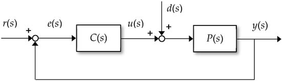
Figure 1. Structure of a basic proportional integral derivative (PID) control system.

Where r(s), y(s), and d(s) denote the set-point input, the process output, and the load disturbance, respectively, e(s) is the error between the reference input and measurement output, and u(s) is the output of controller.

Consider a PIPTD model as shown in Equation (1).

$$P\left(s\right)=\frac{k{e}^{-Ls}}{s}$$

(1)

where L and k represent a time delay and a gain of process, respectively.

The transfer function of the parallel PID controller to be designed is as follows:

$$C\left(s\right)=K_c(1+\frac{1}{T_{i}s}+T_{d}s)$$

(2)

where K_c, T_i and T_d denote a proportional gain, an integral time, and a derivative time of the PID controller, respectively.

The following characteristic equation is obtained from a closed-loop transfer function consisting of a PID controller and IPTD model.

$$1+C\left(s\right)P\left(s\right)=1+\frac{k{e}^{-Ls}}{s}{K}_c(1+\frac{1}{T_{i}s}+T_{d}s)$$

(3)

Using Pade’s approximation, $e^{-Ls}\cong \left(1-0.5Ls\right)/\left(1+0.5Ls\right)$ in Equation (3) is written as

$$1+\frac{k{K}_c{e}^{-Ls}}{s}\left(\frac{T_i{T}_d{s}^2+T_{i}s+1}{T_{i}s}\right)=0$$

(4)

By using the transformation q = Ls in Equation (4), the following dimensionless characteristic equation is obtained.

$$\frac{{\tau }_i{q}^2\left(1+0.5q\right)}{k_c}+\left(1-0.5q\right)\left({\tau }_i{\tau }_d{q}^2+{\tau }_{i}q+1\right)=0$$

(5)

where k_c = kK_c /L, ${\tau }_i$=T_i/L, ${\tau }_d$=T_d/L.

On rearranging Equation (5), Equation (6) is obtained.

$$\left(\frac{{\tau }_i}{2k_c}-\frac{{\tau }_i{\tau }_d}{2}\right)q^3+\left({\tau }_i{\tau }_d-\frac{{\tau }_i}{2}+\frac{{\tau }_i}{k_c}\right)q^2+\left({\tau }_i-\frac{1}{2}\right)q+1=0$$

(6)

In this paper, the desired closed-loop characteristic equation is specified by

$${\left({\tau }_{c}q+1\right)}^3=0,{\tau }_c=T_c/L$$

(7)

Equation (7) comprises three poles located at $-1/{\tau }_c$, and the time constant ${\tau }_c$ of the desired closed-loop transfer function is the tuning parameter. On expanding Equation (7):

$${\tau }_c^3{q}^3+3{\tau }_c^2{q}^2+3{\tau }_{c}q+1=0$$

(8)

The following three equations are obtained by matching the coefficients of $q^3$, $q^2$ Integral of time weighted error and $q$ in Equations (6) and (8).

$$\frac{{\tau }_i}{2k_c}-\frac{{\tau }_i{\tau }_d}{2}-{\tau }_c^3=0$$

(9)

$${\tau }_i{\tau }_d-\frac{{\tau }_i}{2}+\frac{{\tau }_i}{k_c}-3{\tau }_c^2=0$$

(10)

$${\tau }_i-\frac{1}{2}-3{\tau }_c=0$$

(11)

By solving the Equations (9)–(11), three parameters of the PID controller are obtained as follows:

$$k_c=\frac{4\left(6{\tau }_c+1\right)}{{\left(2{\tau }_c+1\right)}^3}$$

(12)

$${\tau }_i=3{\tau }_c+\frac{1}{2}$$

(13)

$${\tau }_d=\frac{-8{\tau }_c^3+12{\tau }_c^2+6{\tau }_c+1}{4\left(6{\tau }_c+1\right)}.$$

(14)

2.2. Set-Point Filter

In the basic PID controller, the error e between the desired value r and the output y of the process is calculated first, the proportional action amplifies the current error, the integrating action amplifies the accumulated error, and the derivative action amplifies the change rate of the error. The proposed PID controller is designed with a focus on load disturbance rejection, so there may be a large overshoot for changes in the desired value. If the overshoot is too large, the control system may become unstable, so set-point filters are used to reduce the overshoot. The PID controller output with the set-point filter is as follows:

$$u\left(t\right)=K_c\left((\mathrm{b}r\left(t\right)-y\left(t\right)+\frac{1}{T_i}{{\displaystyle \int }}_0^t\left(r\left(\tau \right)-y\left(\tau \right)\right)d\tau +T_d\left(\frac{dr\left(t\right)}{dt}-\frac{dy\left(t\right)}{dt}\right)\right)$$

(15)

where u is control input, b is set-point weighting factor with value between 0 and 1.

The Laplace transformation of Equation (15) is given by:

$$u\left(s\right)=K_c\left(1+\frac{1}{T_{i}s}+T_{d}s\right)\left(\frac{T_i{T}_{d}s+\mathrm{b}{T}_{i}s+1}{T_i{T}_{d}s+T_{i}s+1}r\left(s\right)-y\left(s\right)\right)$$

$$=K_c\left(1+\frac{1}{T_{i}s}+T_{d}s\right)\left(F_r\left(s\right)r\left(s\right)-y\left(s\right)\right)$$

(16)

$$F_r\left(s\right)=\frac{T_i{T}_{d}s+\mathrm{b}{T}_{i}s+1}{T_i{T}_{d}s+T_{i}s+1}$$

(17)

The 2-DOF PID control system, in which the set-point filter is considered, is shown in Figure 2.

Figure 2. Structure of 2-DOF (2-degree of freedom) PID control systems with set-point filter.

Where $F_r\left(s\right)$ is the transfer function of the set-point filter, $r\left(s\right)$ and $r_f\left(s\right)$ are the input and output of the set-point filter, respectively.

3. Guideline for Tuning Parameter

MS is used to measure the robustness of proposed PID controller. The definition of MS used as a measure of robustness is as follows:

$$\mathrm{MS}=\begin{array}{c}\max \\ \omega \end{array}\left|\frac{1}{1+C\left(j\omega \right)P\left(j\omega \right)}\right|$$

(18)

where max is the maximum operator and ω represents the angular frequency.

MS is the reciprocal of the nearest distance from critical point to Nyquist curve. Therefore, a large value means that the Nyquist curve is close to the critical point, so it approaches the stability limit. The robustness of the controller is based on MS; the smaller the MS value is, the more robust the controller is said to be in parameter uncertainty, while the larger the value is, the more vulnerable the controller is to parameter change. MS values between 1.4 and 2 for a stable system provide good stability [21]. This value is greater than or equal to 2 for an IPTD system. In Equations (12)–(14), derived from the previous section, the only parameter that needs to be adjusted to tune the PID parameters is a time constant ${\tau }_c$ for the desired characteristic equation. The negative sign to the reciprocal of this adjustable variable becomes the pole in the desired closed-loop transfer function. However, the selection of an appropriate ${\tau }_c$ is also difficult and time consuming. This adjustable parameter should be selected, so that the designed PID controller can give good performance and robustness. Generally, a small value in a stable process results in a faster response as well as better results for load disturbance. However, larger values give the control system more stability or robustness. Therefore, in controller design, it is very convenient to adjust the controller parameters by presenting the values to be adjusted in consideration of stability. Figure 3 shows the change in MS value with respect to the change in ${\tau }_c$ for the PIPTD model.

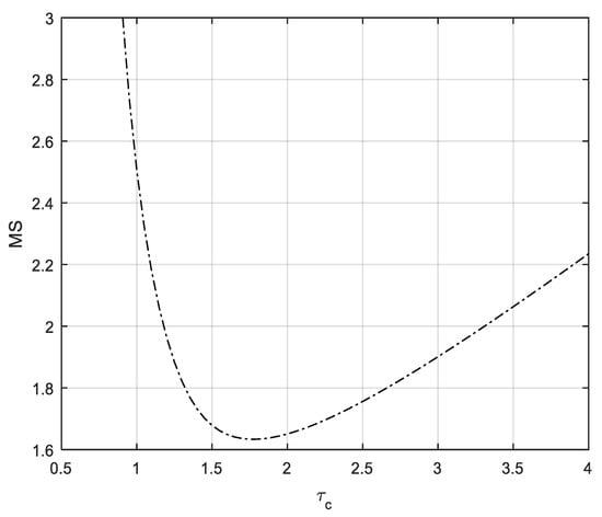
Figure 3. Changes in maximum magnitude of the sensitivity function (MS) for ${\tau }_c$ in the pure integrating processes with time delays (PIPTD) model.

In Figure 3, when time constant ${\tau }_c$ increases to about 1.77, MS is monotonically reduced to about 1.6335, but after that the MS increases again. From Figure 3, the time constant ${\tau }_c$ can be represented as a function of MS using the Matlab Tool Box [25,26,27].

$${\tau }_c=\frac{0.6228{\mathrm{MS}}^2-0.961\mathrm{MS}-0.05428}{{\mathrm{MS}}^2-2.502\mathrm{MS}+1.44}$$

(19)

The value of parameter ${\tau }_c$ should be adjusted according to the MS value selected by the designer, as a trade-off between the response performance and robustness of control system.

4. Simulation

Simulations are performed on three processes to verify the effectiveness of the proposed controller. The servo and regulatory response performance by the proposed method is compared to that of the PID controllers of Jin et al. [13] (hereafter, referred to as Jin), Lee et al. [14] (hereafter, referred to as Lee), and Chidambaram et al. [7] (hereafter, referred to as Chidambaram). For comparisons, performance indices such as 2% settling time t_s, rise time t_r, percentage overshoot (OS [%]), maximum peak error (M_peak), recovery time (t_rcy), and integral of absolute error (IAE) are computed. M_peak represents |r−y_max|, and t_rcy is the time required for the output y to recover to less than 2% of the set-point value after load disturbance is applied. Overall performance is evaluated based on IAE, taking into account other indices of OS [%] etc.

The simulation is performed in two cases for each process. One is the case of a nominal process in which the parameter value of the process has not changed, and the other is when the parameters of the process change by 10% or 20% with respect to the parameters of the nominal process during operation, to verify the robustness of the control system. Assume that there is a 10% or 20% change in the parameter due to uncertainty, but consider the case of the worst conditions. Generally, in PIPTD models, it becomes difficult to control when gain and time delay change to a large side. Therefore, the change in the gain and time delay of the process is simulated, by simultaneously increasing 10% or 20%.

The procedure for tuning the controller is as follows:

• Select a PIPTD model.
• Determine the stability level MS.
• Find the dimensionless time constant from Equation (19).
• Dimensionless k_c, ${\tau }_i$, and ${\tau }_d$ are obtained from Equations (12)–(14).
• K_c, T_i, and T_d are obtained from Equation (5).
• Determine the weighting factor of the set-point filter in Equation (7).

4.1. Process $P_1$

First, the PIPTD model with a relatively small time delay in Equation (1) is considered:

Process $P_1=\frac{0.5e^{-0.4s}}{s}$.

The proposed method is compared to Jin’s method [13] and Lee’s method [14] for this transfer function. The MS value is selected as 2.0, in order to give an impartial comparison. The time constant T_c in the proposed method is tuned to 0.4724, in such a way that the MS value is equal to 2, as given by Jin’s method and Lee’s method. The T_c values in Jin’s method and Lee’s method are 0.7673 and 0.3427, respectively. The weighting factor values b = 0.43, 0.397, and 0.50 are used in the proposed method, Jin’s method, and Lee’s method, respectively. Table 1 summarizes various parameters and MS for process $P_1$.

Table 1. Parameter tuning for process $P_1$.

Tuning Methods	Parameters					MS
	Kc	Ti	Td	Tc	b
Proposed	4.2557	1.6172	0.1440	0.4724	0.43	2.0
Jin	2.8397	1.9345	-	0.7673	0.397	2.0
Lee	2.6929	1.7135	-	0.3427	0.50	2.0

The simulation results for a unit step change in the set-point at t = 0 s and a unit step disturbance input at t = 15 s in the nominal process are presented in Figure 4.

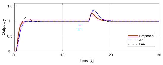
Figure 4. Unit step responses for nominal process $P_1$.

For performance comparisons, the performance indices are listed in Table 2. As shown in Table 2 and Figure 4, Jin’s method shows a similar response to Lee’s method, for regulatory response. The proposed method reduced IAE by about 20%, compared to the other two methods in servo performance, and about 42–44% reduction in regulatory performance. Therefore, the proposed method is significantly better than the other two methods in both servo and regulatory response.

Table 2. Performance comparisons for nominal process $P_1$.

Tuning Methods	Servo Response				Regulatory Response
	tr	ts	OS [%]	IAE	Mpeak	trcy	IAE
Proposed	0.925	2.118	0.301	0.927	0.256	4.316	0.380
Jin	1.212	2.219	0	1.158	0.363	5.559	0.681
Lee	0.941	3.700	11.244	1.152	0.370	3.735	0.650

The robustness is tested on the assumption that the actual process is $P_1=0.6e^{-0.48s}/s$, by simultaneously applying a 20% mismatch in the nominal process parameters. The controller previously designed for nominal process $P_1$ is still used in the simulation. As shown in Figure 5, the overshoot is significantly increased in servo response compared to the nominal process case, but the proposed method represents a shorter t_r and t_s, as well as a smaller IAE, compared to the other two methods. For regulatory response, Lee’s method increases the IAE value significantly compared to the nominal process, but the proposed method has little variation in IAE and provides a shorter t_rcy, a smaller M_peak, and a smaller IAE. These can also be seen in Table 3. The proposed method reduced IAE by about 20–28%, compared to the other two methods in servo response, with about 46–61% reduction in regulatory response. The IAE values are smaller in order of the proposed method, Jin’s method, and Lee’s method. Therefore, the proposed method represents the best performance of the three methods, and Lee’s method shows the worst performance.

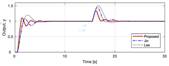
Figure 5. Unit step responses for 20% uncertainty process $P_1$.

Table 3. Performance comparisons for 20% uncertainty process $P_1$.

Tuning Methods	Servo Response				Regulatory Response
	tr	ts	OS [%]	IAE	Mpeak	trcy	IAE
Proposed	0.533	4.202	10.984	1.022	0.337	5.135	0.380
Jin	0.837	4.268	8.09	1.273	0.452	5.485	0.706
Lee	0.936	5.483	20.148	1.428	0.510	5.507	0.969

4.2. Process $P_2$

A process $P_2$ with time delay L = 2, which is five times larger than the time delay of process $P_1$, is considered:

Process $P_2=\frac{0.5e^{-2s}}{s}$.

The proposed method is compared to Jin’s method [13] and Lee’s method [14] for this transfer function. The MS value is selected as 2.0, in order to give a fair comparison. The time constant T_c in the proposed method is tuned to 2.3620, in such a way that the MS value is equal to 2, as given by Jin’s method and Lee’s method. The T_c values in Jin’s method and Lee’s method are 3.8363 and 1.7134, respectively. The weighting factor values b = 0.44, 0.397, and 0.50 of the set-point filter are used in the proposed method, Jin’s method, and Lee’s method, respectively. Table 4 summarizes the various parameters and MS for process $P_2.$

Table 4. Parameter tuning for process $P_2$.

Tuning Methods	Parameters					MS
	Kc	Ti	Td	Tc	b
Proposed	0.8511	8.0860	0.7201	2.3620	0.44	2.0
Jin	0.5679	9.6725	-	3.8363	0.397	2.0
Lee	0.5386	8.5670	-	1.7134	0.50	2.0

Figure 6 shows the simulation results for the unit step change, at set point and unit step disturbance input in the nominal process. For comparisons, the performance indices are tabulated in Table 5. As shown in Table 5 and Figure 6, Jin’s method shows a similar response to Lee’s method in regulatory response. The proposed method reduced IAE by about 20–21% compared to the other two methods in servo response, and about 42–44% reduction in regulatory response. Therefore, the proposed method is significantly better than the other two methods in both servo and regulatory response.

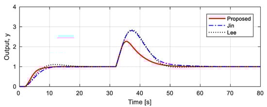
Figure 6. Unit step responses for nominal process $P_2$.

Table 5. Performance comparisons for nominal process $P_2$.

Tuning Methods	Servo Response				Regulatory Response
	tr	ts	OS [%]	IAE	Mpeak	trcy	IAE
Proposed	4.650	10.403	0.374	4.585	1.269	21.613	9.501
Jin	6.176	11.465	0	5.825	1.808	27.678	17.032
Lee	4.766	18.632	10.704	5.733	1.840	18.837	16.239

Robustness is tested on the assumption that the actual process is $P_2=0.6e^{-2.4s}/s$, by simultaneously applying a 20% mismatch in the nominal process parameters. The controller previously designed for nominal process, $P_2$, is still used in the simulation. As shown in Figure 7, the proposed method gives a short t_r, short t_s, and small IAE in servo response, as well as a short t_rcy, small M_peak, and small IAE in regulatory response. These can also be seen in Table 6. The proposed method reduced IAE by about 21–24% compared to the other two methods in servo response, and about 46–47% reduction in regulatory response. The IAE values are smaller in order of the proposed method, Jin’s method, and Lee’s method. Therefore, the proposed method represents the best performance of the three methods, and Lee’s method shows the worst performance.

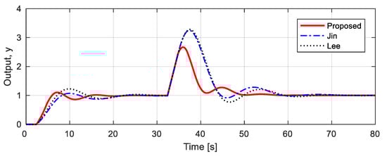
Figure 7. Unit step responses for 20% uncertainty process $P_2$.

Table 6. Performance comparisons for 20% uncertainty process $P_2$.

Tuning Methods	Servo Response				Regulatory Response
	tr	ts	OS [%]	IAE	Mpeak	trcy	IAE
Proposed	2.648	21.039	10.441	4.991	1.668	25.381	9.501
Jin	4.237	21.357	7.15	6.297	2.250	27.430	17.482
Lee	3.570	27.522	22.614	6.566	2.282	28.039	17.907

4.3. Process P₃

A process $P_3$ with time delay L = 6 and k = 0.0506 is considered:

Process $P_3=\frac{0.0506e^{-6s}}{s}$.

The proposed method is compared to Chidambaram’s method [7] for this transfer function. The MS value is selected as 3.82, in order to give a fair comparison. The time constant T_c in the proposed method is tuned to 4.9696, so that it is equal to the MS value of 3.82 taken by Chidambaram’s method. The MS value of 3.82 is too large, and the stability level is low. Therefore, a new MS value of 2.5 is proposed to improve stability. The value of tuning parameter T_c at this time is 6.0030. The value of the coefficient α in Chidambaram’s method is 1.25. Table 7 summarizes the various parameters and MS for process $P_3.$

Table 7. Parameter tuning for process $P_3$.

Tuning Methods	Parameters					MS
	Kc	Ti	Td	Tc or α	b
Proposed 1	3.4138	21.0090	2.3568	6.0030	0.44	2.5
Proposed 2	4.1952	17.9089	2.4263	4.9696	0.3	3.82
Chidambaram	4.0664	27	2.7	1.25 *	0.4	3.82

* 1.25: α value in Chidambaram’s method.

Figure 8 shows the simulation results for the unit step change, at set point and unit step disturbance input in the nominal process. For comparisons, the performance indices are tabulated in Table 8. As shown in Table 8 and Figure 8, Chidambaram’s method shows long t_r, t_s, and t_rcy, as well as large IAE for servo response and regulatory response. The proposed methods are far superior to Chidambaram’s method in both servo and regulatory response.

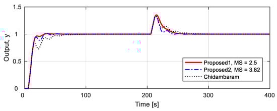
Figure 8. Unit step responses for nominal process $P_3$.

Table 8. Performance comparisons for nominal process $P_3$.

Tuning Methods	Servo Response				Regulatory Response
	tr	ts	OS [%]	IAE	Mpeak	trcy	IAE
Proposed 1	8.904	29.259	0.858	11.994	0.353	55.147	6.154
Proposed 2	8.470	31.166	1.783	12.796	0.331	53.526	4.318
Chidambaram	22.578	61.904	0	16.195	0.328	83.212	6.640

The robustness is tested on the assumption that the actual process is $P_3=0.0556e^{-6.6s}/s,$ by simultaneously applying 10% mismatch in the nominal process parameters. The controller previously designed for nominal process $P_3$ is still used in the simulation. As shown in Table 9 and Figure 9, the proposed method gives a short t_s and small IAE in servo response, as well as a short t_rcy and small IAE in regulatory response. Detailed performance comparisons can also be found in Table 9.

Table 9. Performance comparisons for 10% uncertainty process $P_3$.

Tuning Methods	Servo Response				Regulatory Response
	tr	ts	OS [%]	IAE	Mpeak	trcy	IAE
Proposed 1	7.036	42.387	9.693	12.996	0.411	63.281	6.155
Proposed 2	6.747	91.927	12.008	16.681	0.389	110.565	6.820
Chidambaram	7.116	102.772	4.883	17.793	0.386	112.515	7.266

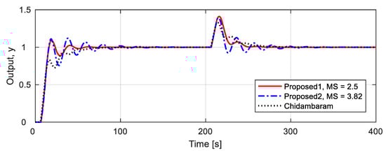
Figure 9. Unit step responses for 10% uncertainty process $P_3$.

5. Discussion

In this section, the effect of the set-point filter, changes in load disturbance rejection performance according to MS values, and stability of parameter uncertainty are examined.

5.1. Effect of Set-Point Filter

Since the proposed technique focuses on improving regulatory performance, there may be a significant overshoot for step changes in set-point. Set-point filter may be used to mitigate overshoots in servo response. To verify performance improvement by using set-point filter, the process $P_1=0.5e^{-0.4s}/s$ has been considered. The controller previously designed for nominal process $P_1$ is still used in the simulation. If the filter weighting factor is b = 1.0, the transfer function of the set-point filter becomes 1 and the filter is not used, and if the filter weighting factor is b = 0.43, then the transfer function of the set-point filter is expressed as $F_r\left(s\right)=\left(T_i{T}_d{s}^2+0.43T_{i}s+1\right)/\left(T_i{T}_d{s}^2+T_{i}s+1\right)$. Figure 10 shows the unit step response by the proposed controller with and without a set-point filter, and Table 10 summarizes the performance indices such as t_r, t_s, OS [%], M_peak, t_rcy, and IAE. Using a set-point filter of b = 0.43 reduces the IAE value from 1.246 to 0.927, OS [%] from 43.896 to 0.301, and settling time from 4.071 to 2.118. As expected, the use of the set-point filter can improve the performance of servo response. In addition, Table 10 confirms that the set-point filter does not affect regulatory response at all.

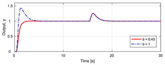
Figure 10. Unit step responses with and without set-point filter for nominal process $P_1$.

Table 10. Effect of set-point filter for nominal process $P_1$.

Set-Point Filter	Servo Response				Regulatory Response
	tr	ts	OS [%]	IAE	Mpeak	trcy	IAE
With filter	0.925	2.118	0.301	0.927	0.256	4.316	0.380
Without filter	0.332	4.071	43.896	1.246	0.256	4.316	0.380

5.2. Changes in Load Disturbance Rejection Performance According to MS Values

When designing a controller, it is necessary to make a reasonable compromise between stability (or robustness) and control performance. In this paper, MS was used as a measure of stability. The response performance change, according to MS values, is tested considering the process $P_2=0.5e^{-2s}/s$, as discussed in the previous section. Controllers are designed for MS values of 1.7, 2.0, and 2.3, with stability levels by the proposed method. Table 11 summarizes the desired time constant T_c and PID controller parameters, according to MS.

Table 11. Parameter tuning for process $P_2$, according to MS values.

Tuning Methods	Parameters
	Kc	Ti	Td	Tc	b
Proposed, MS = 1.7	0.6475	9.7660	0.5341	0.9220	0.44
Proposed, MS = 2.0	0.8511	8.0861	0.7201	2.3620	0.44
Proposed, MS = 2.3	0.9736	7.3361	0.770	2.1120	0.44

The simulation results for the unit step change in set point at t = 0 s and the unit step disturbance input at t = 100 s are presented in Figure 11. Values for the various evaluation indices for quantitative comparison are presented in Table 12. For in servo and regulatory response, it can be seen that the higher the MS values result in greater OS [%], but decreases t_r, t_s, IAE, M_peak, and t_rcy. Therefore, it can be said that as the MS value increases, the response speed increases, but the stability deteriorates.

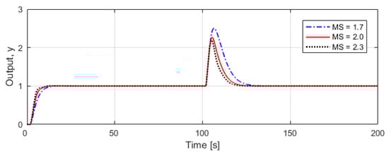
Figure 11. Unit step responses according to MS for nominal process $P_2$.

Table 12. Performance comparisons for nominal process $P_2$ according to MS.

Tuning Methods	Servo Response				Regulatory Response
	tr	ts	OS [%]	IAE	Mpeak	trcy	IAE
Proposed, MS = 1.7	6.595	12.781	0.298	5.522	1.503	26.758	15.083
Proposed, MS = 2.0	4.650	10.403	0.374	4.585	1.269	21.613	9.501
Proposed, MS = 2.3	3.426	9.806	0.547	4.174	1.194	19.325	7.535

5.3. Verification of Stability against Parameter Uncertainty

In the simulation in the previous section, a parameter uncertainty of 10% was taken into account for process $P_3$. At 10% parameter uncertainty, Chidambaram’s method did not give satisfactory control performance, but stabilized over time. This time, assuming a parameter uncertainty of 20.5%, a unit step input was applied at t = 0 s, and a unit load disturbance was applied at t = 400 s. In the simulation, the same controllers were used that were designed earlier, in both cases. The step responses and control inputs are shown in Figure 12. Values for various evaluation indices for quantitative comparison are presented in Table 13. The proposed method has a slightly worse control performance than in the case of 10% parameter uncertainty, but in Chidambaram’s method, the response is unstable, and no value other than the rise time can be represented. Therefore, it can be confirmed that the proposed method is significantly stronger against parameter uncertainty than Chidambaram’s method.

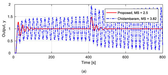
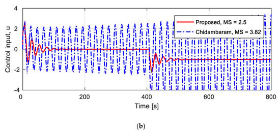
Figure 12. Unit step responses and control inputs for 20.5% uncertainty process $P_3$. (a) Unit step responses; (b) control inputs.

Table 13. Performance comparisons for 20.5% uncertainty process $P_3$.

Tuning Methods	Servo Response				Regulatory Response
	tr	ts	OS [%]	IAE	Mpeak	trcy	IAE
Proposed, MS = 2.5	6.066	105.319	27.614	19.562	0.478	115.497	8.984
Chidambaram, MS = 3.82	5.918	unstable	unstable	unstable	unstable	unstable	unstable

6. Conclusions

In this paper, a 2-DOF PID controller based on the DS method was proposed to simultaneously improve servo and regulatory response for PIPTD models, and how to tune the PID parameters was discussed. The 2-DOF PID controller consists of a linear PID controller for rejecting load disturbance in regulatory response and a set-point filter for mitigating the overshoot in servo response, while the controller design was more focused on improving regulatory responses.

As the key contribution of this paper, by placing the roots of the desired characteristic equation at the same location, the adjustment parameter is only one desired time constant, and the desired time constant was expressed as a function of MS, to provide convenience in the selection of the desired time constant. Therefore, controller design and parameter tuning by the proposed method can be performed very easily. To demonstrate the feasibility of the proposed method, simulations were performed on three PIPTD processes and compared with the results of the three existing methods.

Although there are differences depending on the processes, the proposed method reduced IAE by about 20–21%, compared to the other two methods’ in servo response for the nominal process, and decreased IAE by about 42–44% in regulatory response. In the case of parameter uncertainty, the proposed method decreased IAE by about 20–28%, compared to the other two methods’ in servo response, and about 46–61% reduction in regulatory response. In addition, the effect of the set-point filter, performance change according to MS, and stability, due to parameter uncertainty, were examined.

By using set-point filters, the overshoot was reduced from 44% to 0.3%, and IAE was reduced by 26% compared with no set-point filter. It was confirmed that the larger the MS value is, the faster the response speed, but the stability decreased. The PID controller by the proposed method was robust against the parameter uncertainty of the process. The proposed method was confirmed to be effective in both servo and regulatory responses.

Future studies will continue research on first order systems, plus a time delay with an integrator, second order systems plus a time delay, and systems with time delays that take into account a saturator.

References

- O’Dwyer, A. Handbook of PI and PID Controller Tuning Rules; Imperial College Press: London, UK, 2009. [Google Scholar]
- Pathiran, A.R.; Prakash, J. Design and implementation of a model-based PI-like control scheme in a reset configuration for stable single-loop systems. Can. J. Chem. Eng. 2014, 92, 1651–1660. [Google Scholar] [CrossRef]
- Tavakoli, S.; Tavakoli, M. Optimal tuning of PID controller for first order plus time delay models using dimensional analysis. In Proceedings of the Fourth International Conference on Control and Automation, Montreal, QC, Canada, 12 June 2003; pp. 942–946. [Google Scholar]
- Cvejn, J. Sub-optimal PID controller settings for FOPDT systems with long dead time. J. Process Control 2009, 19, 1486–1495. [Google Scholar] [CrossRef]
- Luyben, W.L. Design of proportional integral and derivative controllers for integrating dead-time processes. Ind. Eng. Chem. Res. 1996, 35, 3480–3483. [Google Scholar] [CrossRef]
- Kookos, I.K.; Lygeros, A.I.; Arvanitis, K.G. On-line PI controller tuning for integrator/dead time processes. Eur. J. Control 1999, 5, 19–31. [Google Scholar] [CrossRef]
- Chidambaram, M.; Sree, R.P. A simple method of tuning PID controllers for integrator/dead-time processes. Comput. Chem. Eng. 2003, 27, 211–215. [Google Scholar] [CrossRef]
- Sree, R.P.; Chidambaram, M. A Simple and Robust Method of Tuning PID Controllers for Integrator/Dead Time Processes. J. Chem. Eng. Jpn. 2005, 38, 113–119. [Google Scholar] [CrossRef]
- Ali, A.; Majhi, S. Integral criteria for optimal tuning of PI/PID controllers for integrating processes. Asian J. Control 2010, 13, 328–337. [Google Scholar] [CrossRef]
- Anil, C.; Sree, R.P. Design of optimal PID controllers for integrating systems. Indian Chem. Eng. 2014, 56, 215–228. [Google Scholar] [CrossRef]
- Jin, G.-G.; Son, Y.-D. Design of a Nonlinear PID Controller and Tuning Rules for First-Order Plus Time Delay Models. Stud. Inform. Control 2019, 28, 157–166. [Google Scholar] [CrossRef] [Green Version]
- Skogestad, S. Simple analytic rules for model reduction and PID controller tuning. J. Process Control 2003, 13, 291–309. [Google Scholar] [CrossRef] [Green Version]
- Jin, Q.; Liu, Q. Analytical IMC-PID design in terms of performance/robustness tradeoff for integrating processes: From 2-Dof to 1-Dof. J. Process Control 2014, 24, 22–32. [Google Scholar] [CrossRef]
- Lee, J.; Cho, W.; Edgar, T.F. Simple Analytic PID Controller Tuning Rules Revisited. Ind. Eng. Chem. Res. 2013, 53, 5038–5047. [Google Scholar] [CrossRef]
- Shamsuzzoha, M. A unified approach for proportional-integral-derivative controller design for time delay processes. Korean J. Chem. Eng. 2015, 32, 583–596. [Google Scholar] [CrossRef]
- Ahmadi, A.H.; Nikravesh, S.K.; Amani, A.M. A Unified IMC based PI/PID controller tuning approach for time delay processes. AUT J. Electr. Eng. 2020, 52, 31–52. [Google Scholar] [CrossRef]
- Li, Z.; Bai, J.; Zou, H. Modified two-degree-of-freedom Smith predictive control for processes with time-delay. Meas. Control 2020, 53, 691–697. [Google Scholar] [CrossRef] [Green Version]
- Chen, D.; Seborg, D.E. PI/PID Controller Design Based on Direct Synthesis and Disturbance Rejection. Ind. Eng. Chem. Res. 2002, 41, 4807–4822. [Google Scholar] [CrossRef]
- Rao, A.S.; Rao, V.S.R.; Chidambaram, M. Direct synthesis-based controller design for integrating processes with time delay. J. Frankl. Inst. 2009, 346, 38–56. [Google Scholar] [CrossRef]
- Ajmeri, M.; Ali, A. Direct synthesis based tuning of the parallel control structure for integrating systems. Int. J. Syst. Sci. 2015, 46, 2461–2473. [Google Scholar] [CrossRef]
- Anil, C.; Sree, R.P. Tuning of PID controllers for integrating systems using direct synthesis method. ISA Trans. 2015, 57, 211–219. [Google Scholar] [CrossRef]
- Yerolla, R.; Besta, C.S. Development of tuning free SISO PID controllers for First Order Plus Time Delay (FOPTD) and First Order Lag Plus Integral Plus Time Delay model (FOLIPD) systems based on partial model matching and experimental verification. Results Control Optim. 2021, 5, 100070. [Google Scholar] [CrossRef]
- Korkmaz, M.; Aydogdu, O.; Dogan, H. Design and performance comparison of variable parameter nonlinear PID controller and genetic algorithm based PID controller. In Proceedings of the 2012 International Symposium on Innovations in Intelligent Systems and Applications (INISTA 2012), Trabzon, Turkey, 2–4 June 2012; pp. 1–5. [Google Scholar]
- So, G. Design of an Intelligent NPID Controller Based on Genetic Algorithm for Disturbance Rejection in Single Integrating Process with Time Delay. J. Mar. Sci. Eng. 2020, 9, 25. [Google Scholar] [CrossRef]
- Curve Fitting Toolbox. In User’s Guide; Mathworks: Natick, MA, USA, 2020.
- System Identification Toolbox. In Getting Started Guide; Mathworks: Natick, MA, USA, 2020.
- System Identification Toolbox. In User’s Guide; Mathworks: Natick, MA, USA, 2020.
Publisher’s Note: MDPI stays neutral with regard to jurisdictional claims in published maps and institutional affiliations. |
© 2022 by the author. Licensee MDPI, Basel, Switzerland. This article is an open access article distributed under the terms and conditions of the Creative Commons Attribution (CC BY) license (https://creativecommons.org/licenses/by/4.0/).