Calibration of Hydrodynamic Models of Groundwater Flow in Aquifers Polluted by Liquid Radioactive Waste

Abstract

Pollution of aquifers by liquid radioactive waste is especially hazardous due to high permeability of aquifer rocks. Pollution can take place as a result of deep injection disposal of liquid waste or due to its leakage from a surface reservoir. The ecological hazard depends on distribution of aquifer permeability, which can be highly heterogeneous. The only source of data for determination of such distribution is measurements in exploratory boreholes at the polluted site. A technique is proposed for determination of spatial distribution of aquifer transmissibility on the basis of hydrological measurements in a limited number of boreholes. The problem is reduced to a minimization problem which was solved numerically.

1. Introduction

As it follows from some estimations [1,2], operation of all atomic power plants over the world leads to production of ≅11,300–11,500 t of spent nuclear fuel (SNF) per year. With a fuel cycle involving reprocessing and potential recycling of plutonium, SNF is dispatched after extraction from a reactor to radiochemical plants for reprocessing. Processing of 1 t of SNF leads to production of 13–34 m³ of liquid radioactive waste (LRW) [3] with activity of more than 10 Ci/l [4].

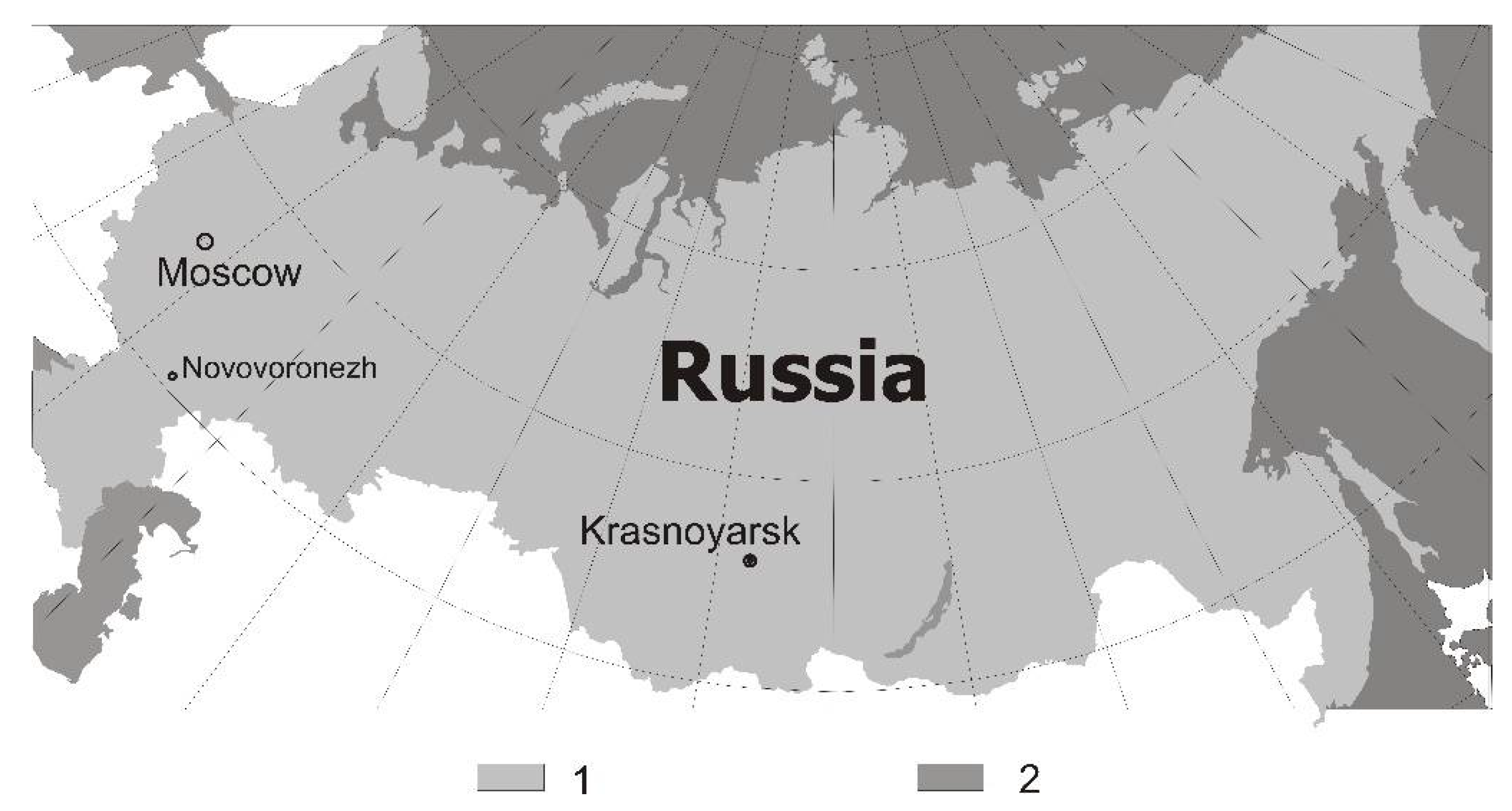
In the USSR and later in Russia, deep injection of LRW was carried out on an industrial scale. LRW was injected into deep-seated, highly permeable aquifers confined from top and bottom by low permeable rocks. Such injection technology was implemented for disposal of LRW from the Mining and Chemical Plant in the Krashoyarsk region [5] (Figure 1).

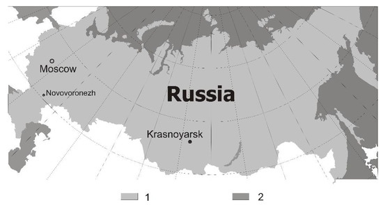
Figure 1. Location of Novovoronezh and Krasnoyarsk. (1) Territory of Russian Federation; (2) seas and lakes.

Reprocessing of SNF is not the only source of LRW, which can be produced also from maintenance of operation of atomic power plants. This LRW is usually accumulated at territories of the power stations in special reservoirs. As a result of an emergence, LRW can gush out from the reservoir to the earth’s surface and then move with groundwater in the upper free aquifer to the zone of groundwater discharge, to an open reservoir or a river. An example of such radioactive pollution was an accident at the atomic power plant (APP) Novovoronezhskaya in 1985 [6].

In both cases, a radioactive plume moves from a pollution source to the biosphere through a permeable sedimentary rock layer thickness which is much less than its areal dimensions.

Assessment of an ecological hazard of radionuclides released to the biosphere calls for calculation of groundwater stream velocities. The key parameter in this calculation is spatially distributed water transmissivity of the aquifer rocks [7]. The only source of input data for determination of this distribution is data of transmissivity measurements in observation boreholes which are drilled at the pollution site. Since drilling of such boreholes is rather expensive (especially in a case of a deep-seated aquifer), the amount of measurement data is limited. A calibration of a mathematical model of groundwater flow in the aquifer is a determination of such spatial distribution of water transmissivity of the aquifer, which is consistent with hydrological measurements in the observation boreholes.

2. Description of the Pollution Sites

2.1. Deep Injection Site of the Mining and Chemical Plant

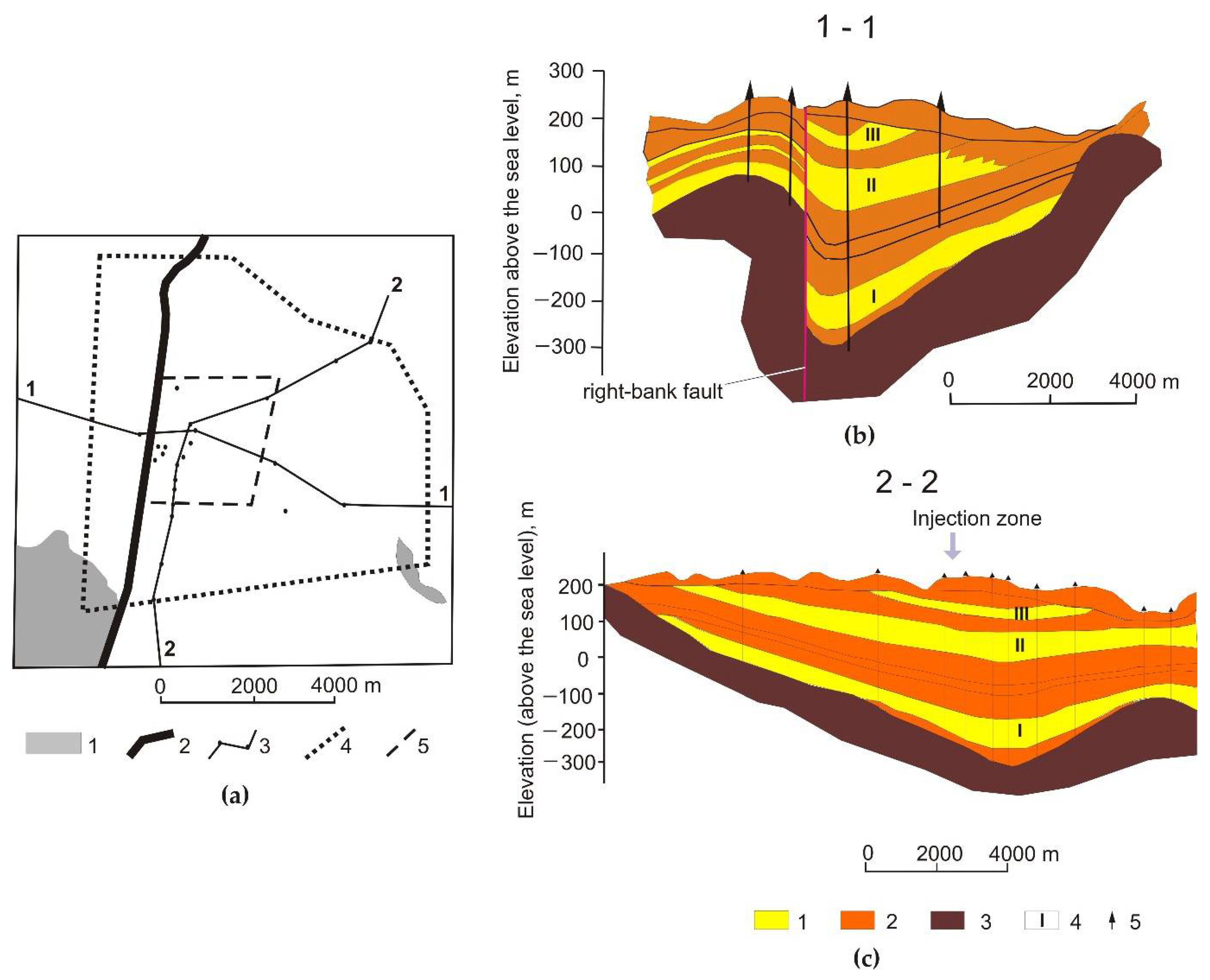
There are (1) highly permeable sandy aquifers (Horizons I, II, and III), (2) low-permeability clayey aquitards, (3) basement rocks, (4) a Horizon index, and (5) exploratory wells.

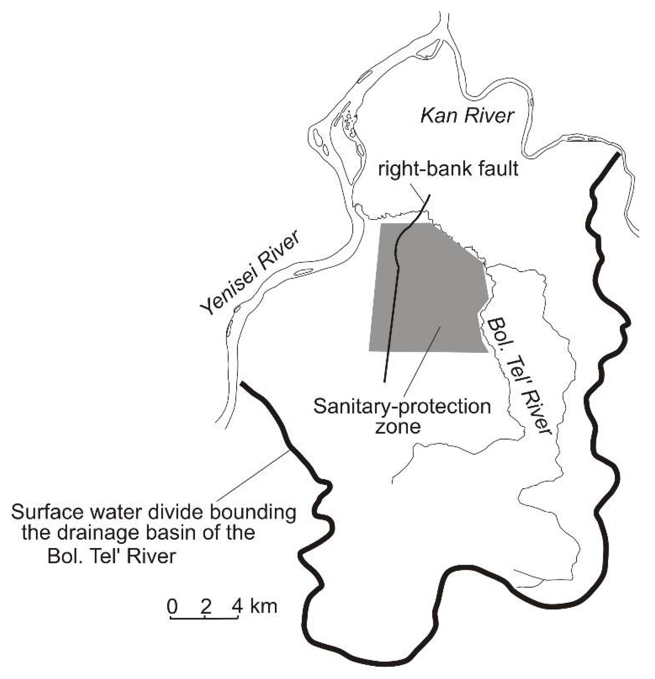
The deep injection site for disposal of LRW from MCP is located on the eastern bank of the river Yenisei in the Krasnoyarsk region (Figure 2). The geological medium in the injection domain is represented by a small-size sedimentary basin. It is built up by a layered clay–sandy Jurassic sequence with the maximum thickness of 550 m, which fills an erosional paleovalley in the Pre-Cambrian crystalline basement. Three (sandy to weakly cemented sandstone) aquifers are relatively clearly defined in the geological section of the sedimentary sequence (Figure 3) and are labeled from bottom to top as Horizons I, II, and III. The lowest aquifer (Horizon I) is confined from bottom by low-permeability basement rocks.

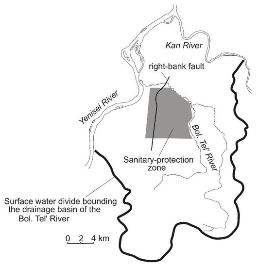
Figure 2. Location of the injection site for the disposal of LRW from MCP.

Figure 3. Cross-sections of the underground medium at the injection site for disposal of LRW from MCP after [5]. (a) Schematic diagram of the injection site; (1) basement rocks, (2) right-bank fault, (3) cross-section lines and exploratory wells, (4) boundary of the sanitary protection zone, and (5) boundary of the LRW disposal site. (b,c) Schematic hydrogeological cross-sections along the lines 1-1 and 2-2 (see (a)).

The layered sequence is truncated both structurally and hydraulically by a subvertical tectonic fault zone (right-bank fault) (Figure 3a). This fault is traced for a distance of about 2 km to the north and south of the sanitary-protection zone. Uplift of the block of the basement rock to the west of the fault seals Horizon I from the west (Figure 3c) and separates the waste plume in Horizon I from the Yenisei river.

Intermediate-level LRW (with radioactivity up to 10⁻² Ci/liter) are injected into Horizon I. From 1972 to 1993, Horizon I has been used also for disposal of LRW with elevated radioactivity (up to 5 Ci/l) [5].

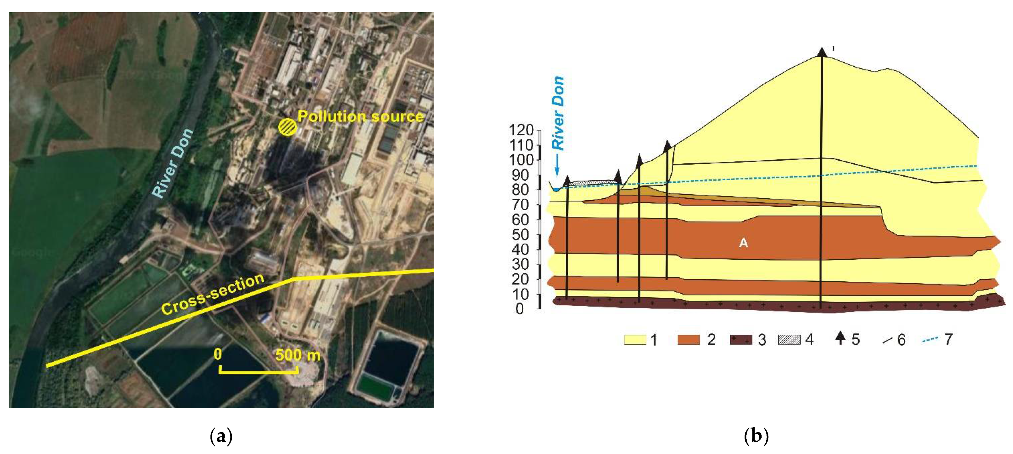
2.2. Pollution Site at Atomic Power Plant Novovoronezhskaya

Pollution of groundwater with ⁶⁰Co at the site of APP Novoronezhskaya is caused by a leakage of concentrated technological LRW from a temporary storage in 1985. Estimated volume of the leakage was 480 m³, and activity of ⁶⁰Co in LRW at the time of the leakage was 1.34 × 10¹¹ Bq/m³ [6].

APP and its temporary storage of LWR are located on the left bank of the river Don (Figure 4a). The upper part of the underground medium at the site of APP is represented by a layered sequence of clayey–sandy sedimentary deposits confined from the bottom by tight basement rocks (Figure 4b). The contaminant plume moves within two upper aquifers above the argillaceous layer which is denoted with letter A in Figure 4b. As it is seen in (Figure 4b) they are partially divided from each other by a clayey interlayer, however they have a structural and hydrologic connection, as is shown in Figure 4b. An important argument in favor of this statement is very smooth relief of the water table (Figure 4b).

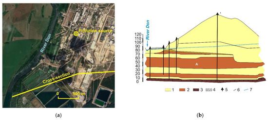
Figure 4. Pollution site at the APP Novovoronezhskaya. (a) Location of the pollution site (from Google satellite photograph). (b) Vertical cross-section of the pollution site (after data from enterprise “Gydrospetsgeologiya”). (1) highly permeable sedimentary deposits; (2) low-permeability clayey rocks; (3) tight basement rocks; (4) Quaternary deposits; (5) exploratory boreholes; (6) boundaries between sedimentary deposits of different origin; (7) water table.

3. Technique of Calibration of Hydrologic Models

3.1. Confined Aquifer Example of the Injection Site of LRW from Mining and Chemicals Combined

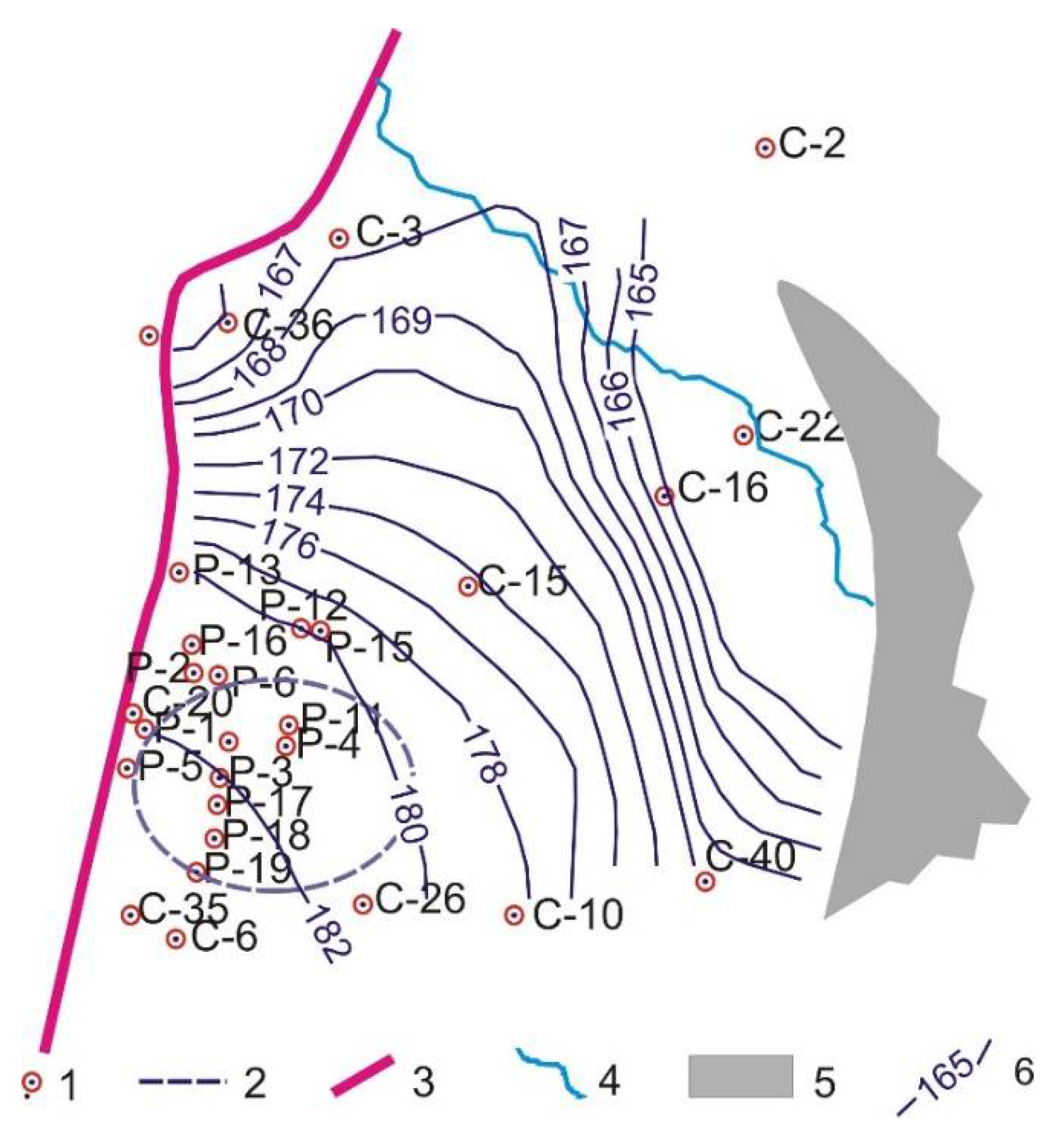
If thickness of an aquifer is much less than its areal dimensions (it should be taken into account that horizontal scales in Figure 3b,c differ approximately by an order of magnitude from the vertical scale), a 2D planar approximation is quite sufficient for determination of groundwater flow in the aquifer. In a case of a confined aquifer, measurement data include values of hydraulic head in the observation boreholes and values of aquifer transmissibility, obtained by pumping tests in a part of the boreholes (Figure 5). The calibration problem reduces to determination of such spatial distribution of transmissibility that measured transmissibility coincides with the corresponding local value of the distribution, and values of hydraulic head, which are calculated on the basis of this distribution, and are in good agreement with the measured values.

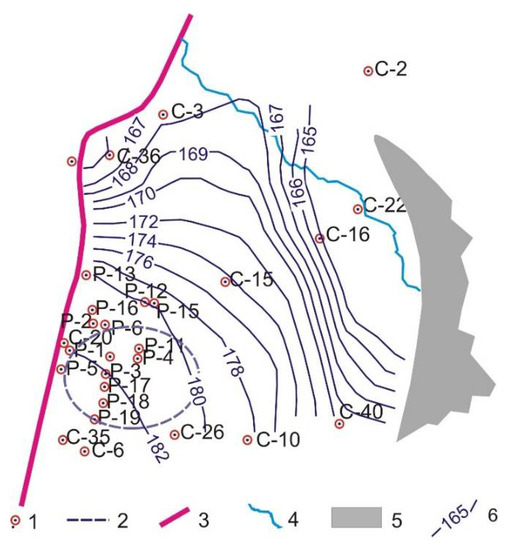
Figure 5. Exploratory borehole locations at the deep injection site of MCP. (1) Boreholes; (2) injection site; (3) right-bank fault; (4) river; (5) zone of wedging out of Horizon I; calculated levels of hydraulic head in Horizon I.

Let us consider an areal model of groundwater flow in Horizon I, taking into account a leakage between Horizons I and II. Pumping tests and hydraulic head measurements were carried before injection. Salinity of the groundwater was uniform at that time. Hence, buoyancy forces caused by heterogeneity of the groundwater density were absent at that time. Then velocity components satisfied Darcy’s law in the form

$$v_x=-f\frac{\partial H_1}{{\partial }_x},\hspace{1em}{v}_y=-f\frac{\partial H_1}{{\partial }_y}$$

(1)

where $f=f(x,y)$ is hydraulic conductivity of rock in Horizon I, and $H_1=H_1(x,y)$ is hydraulic head in Horizon I.

The equation of water balance in Horizon I can be written in the form

$$\frac{\partial (\delta v_x)}{\partial x}+\frac{\partial (\delta v_y)}{\partial y}=-q$$

(2)

where $\delta =\delta (x,y)$ is thickness of Horizon I; $q=q(x,y)$ is volume of groundwater which flows through unit square of the upper boundary of Horizon I per unit time (positive at ascending leakage).

According to [7], the value of $q$ can be represented as

$$q=\sigma (H_1-H_2)$$

(3)

where $H_2=H_2(x,y)$ is hydraulic head in Horizon II; $\sigma =\sigma (x,y)$ is parameter of the leakage between Horizons I and II.

$$\sigma =\frac{f_{tr}}{\Delta }$$

Here, $f_{tr}=f_{tr}(x,y)$ is hydraulic conductivity of the low-permeability clayey layer between Horizons I and II; $\Delta =\Delta (x,y)$ is thickness of the layer.

Substitution of (1) and (3) into (2) gives

$$\frac{\partial }{\partial x}\left(W\frac{\partial H_1}{\partial x}\right)+\frac{\partial }{\partial y}\left(W\frac{\partial H_1}{\partial y}\right)=\sigma (H_1-H_2),\hspace{1em}\hspace{1em}x,\hspace{0.17em}y\in \Omega$$

(4)

where $W=\delta f$ is transmissibility of Horizon I, and $\Omega$ is modeling domain.

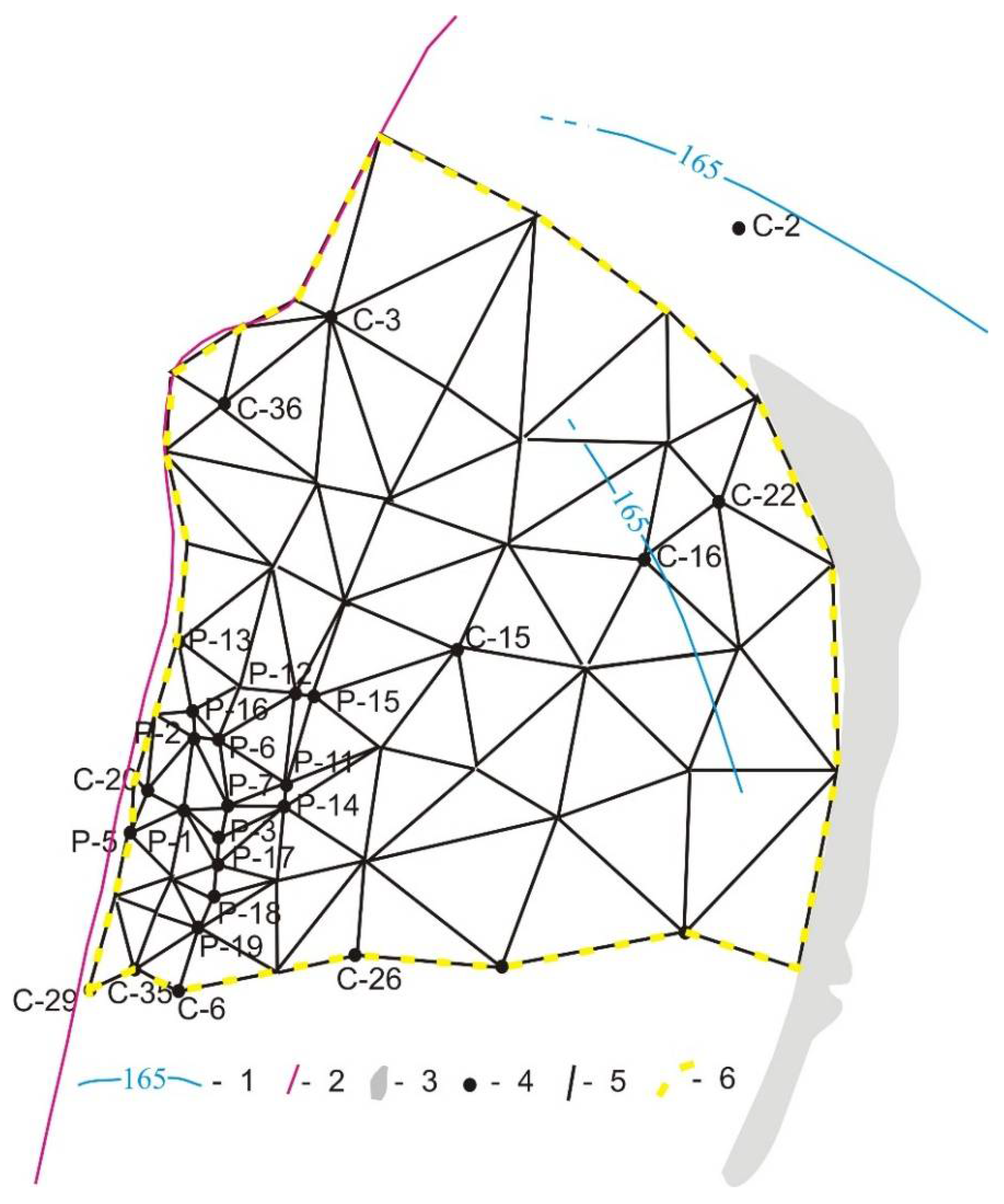
Let us specify $\Omega$ as it is shown with a yellow dashed line in Figure 6.

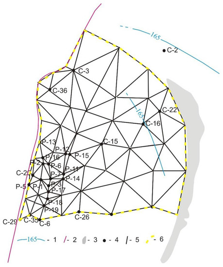
Figure 6. Modeling domain with finite elements. (1) Level of hydraulic head; (2) right-bank fault, (3) zone of wedging out of Horizon I; (4) boreholes; (5) boundaries of finite elements; (6) boundary of the modeling domain.

As it follows from Figure 3b, the right-bank fault forms an impermeable boundary for the part of Horizon I to the east of the fault. The zone of wedging out of Horizon I is also impermeable. Hence, we can specify zero Neumann conditions at the eastern and western boundaries of $\Omega$. As it follows from measurements of hydraulic head in observation boreholes, the gradient of hydraulic head at the northern boundary is low (Figure 6). This allows consideration of two practically identical variants of boundary conditions at the northern boundary of $\Omega$:

• Dirichlet conditions: $H_1$ = 165 m;
• Zero Neumann conditions.

Values of $H_1$ at the southern boundary of $\Omega$ are determined by piece–linear interpolation of values, which are measured in observation boreholes.

Data of measurements in the boreholes within $\Omega$ consist of $N$ values of hydraulic head in $N$ points of $\Omega$.

$$\{H_1(x_i^H,y_i^H)=h_i,\hspace{1em}\hspace{1em}i=1,\dots ,N\}$$

(5)

$M$ values of transmissibility in $M$ points of $\Omega$:

$$\{W(x_j^W,y_j^W)=W_j^{meas},\hspace{1em}\hspace{1em}j=1,\dots ,M\}$$

(6)

Let us denote $\left\{W\right\}$ an aggregate of distributions, $W(X,Y)$ which satisfies conditions (6), and corresponding solutions of (4) satisfy conditions (5) at specified $H_2$ and conditions at the boundary of $\Omega$. It is possible that such a distribution is not unique, and $\left\{W\right\}$ consists of several elements (or even of infinite number of them). Hence, a problem emerges to specify an additional condition for selection of a unique element from $\left\{W\right\}$.

A characteristic feature of aquifers from unconsolidated sediments in layered sequences is relatively smooth variation of their hydraulic transmissivity on macroscale in horizontal directions, in comparison with hydraulic conductivity variations on a microscale [8]. As a condition for selection of a unique element from $\left\{W\right\}$, this can be written in the form

$$\Phi (W)={\displaystyle \underset{\Omega }{\iint }\left[{\left(\frac{\partial W}{\partial x}\right)}^2+{\left(\frac{\partial W}{\partial y}\right)}^2\right]\hspace{0.17em}dx\hspace{0.17em}dy}\to \min$$

(7)

Therefore, the calibration problem is reduced to a search of a conditional minimum of the functional $\Phi \left(W\right)$. In the considered case, the problem can be solved only numerically.

Independently of the method of numerical solution of Equation (4), it is desirable from the viewpoint of accuracy to use a grid where points $\{(x_i^H,y_i^H),\hspace{1em}\hspace{0.33em}i=1,\dots ,N\}$ and $\{(x_j^W,y_j^W),\hspace{1em}\hspace{0.33em}j=1,\dots ,M\}$ are nodes. As it is seen in Figure 5, points of boreholes are distributed in an irregular manner, and use of finite-difference methods with a rectangular grid is complicated. That is why we used a finite-element method [9].

Let us denote the vector of nodal values of $H_1$ as $H_1$. If we use a weak Galerkin finite-element method [9,10], the boundary problem for Equation (4) takes the form

$$A{H}_1=0$$

(8)

$A$ is a symmetric positively definite matrix what allows the solving of Equation (8) with the fast Cholesky method [11].

With use of finite-element approximation, the distribution $W$ is fully determined through a vector of nodal values of $W$, and the functional $\Phi$ takes the form

$$\Phi (W)={\displaystyle \sum S_{i\hspace{0.17em}j}{W}_i{W}_j}$$

(9)

where $W$ is vector of nodal values, $W_i$, and $S$ is a symmetric positively defined matrix.

Conditions (5) and (6) take the form

$$H_{I_n}=h_n,\hspace{1em}\hspace{0.33em}n=1,\dots ,N;\hspace{1em}\hspace{1em}\hspace{1em}{W}_{J_m}=W_m^{meas},\hspace{0.33em}\hspace{1em}m=1,\dots ,M$$

(10)

where $I_n,\hspace{0.33em}{J}_m$ are a numbers of nodes corresponding to boreholes with numbers $n$ and $m$, respectively.

Hence, the calibration of the model of groundwater flow reduces to the search of a maximum of the quadratic form (9) at conditions (8) and (10), i.e., to a search for a conditional minimum in classic formulation.

Direct methods of search for an extremum with implicitly defined conditions are not obvious. That is why the problem was solved by an approximate method with use of a penalty function [12], and we determined an unconditional minimum of the functional

$${\Phi }^{*}(W)=\Phi (W)+G\left[{\displaystyle \sum _{n=1}^N{(H_{I_n}-h_n)}^2}+{\displaystyle \sum _{m=1}^M{(W_{J_m}-W_m^{meas})}^2}\right]$$

(11)

where $G$ is a parameter. The calculations were carried out at increasing $G$, up to such a value that the variation of $W$ at future growth of $G$ does not exceed 5%.

Since points of boreholes $\{(x_j^W,y_j^W),\hspace{1em}\hspace{0.33em}j=1,\dots ,M\}$ are nodes of finite elements, values of $W(x_j^W,y_j^W)$ are fixed and equal to measured values. Hence, the second sum in the square brackets in the right-hand side of the expression (11) is equal to zero.

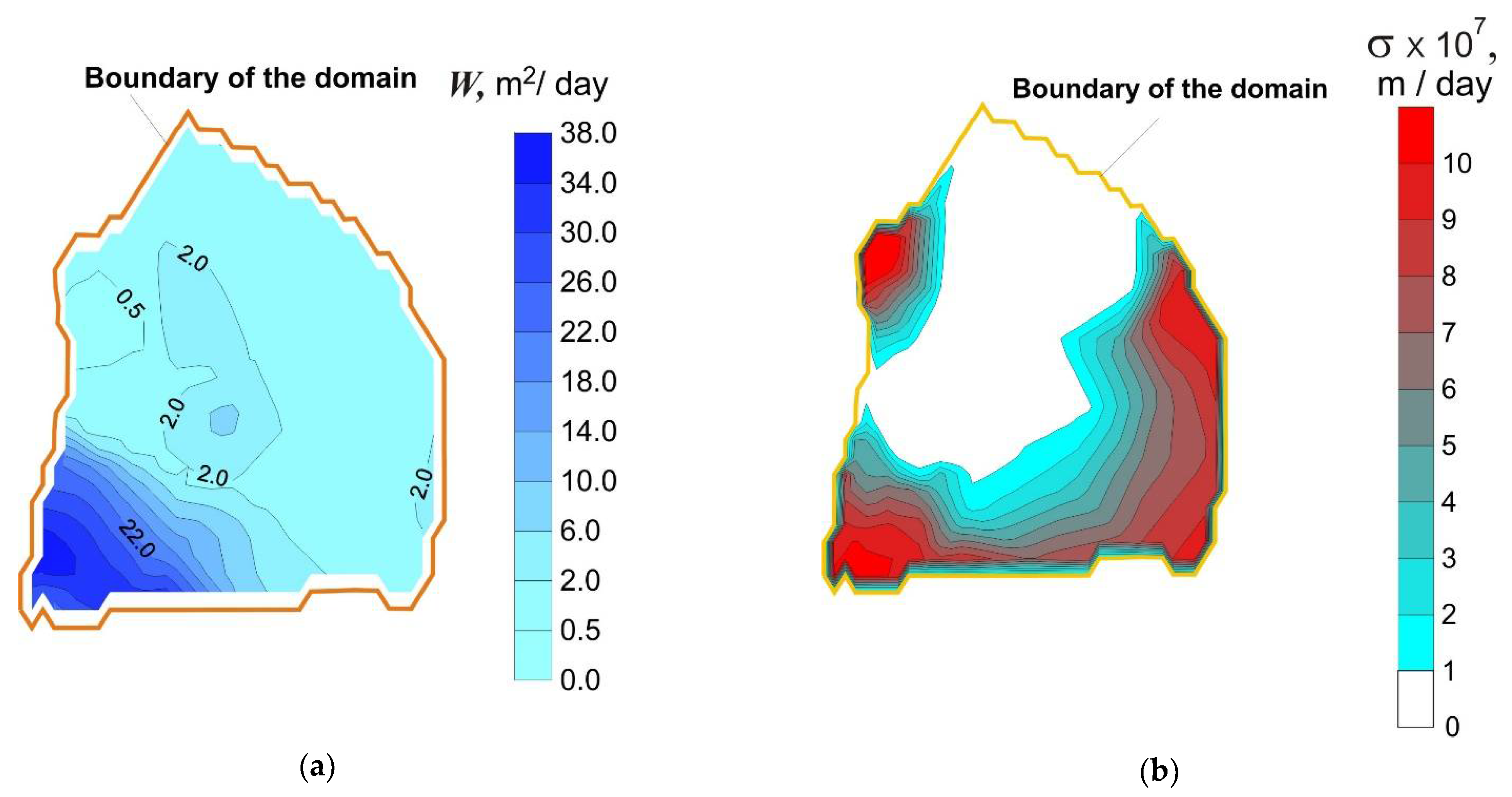
A minimum of (11) was determined by a modified method of gradient minimization. Obtained distributions of $W$ and $\sigma$ are presented in Figure 7.

Figure 7. Distributions of $W$ (a) and $\sigma$ (b).

Calculated values of $W$ at the points of boreholes are equal exactly to measured values. A comparison of calculated and measured values of $H_1$ is presented in Table 1.

Table 1. Comparison of calculated and measured values of hydraulic head in Horizon I in the points of boreholes.

Number of Borehole	Measured Value of H1, m	Calculated Value of H1, m
P-1	182.25	182.04
P-2	182.10	181.63
P-3	182.28	182.10
P-5	182.59	182.37
P-12	181.42	180.46
P-13	181.31	180.97
C-3	167.78	167.65
C-6	183.73	183.73
C-10	178.81	178.81
C-15	174.17	174.50
C-16	165.53	165.53
C-22	160.49	160.51
C-36	165.75	165.89
C-40	169.90	169.90

One can see that calculated and measured values of $H_1$ are in a satisfactory agreement.

3.2. Free Aquifer Example of the Pollution Site at APP Novovoronezhskaya

The aquifer is confined from its bottom by practically impermeable argillaceous deposits. Atmospheric precipitations enter the aquifer through its upper free boundary. The balance equation in this case takes the form

$$\frac{\partial }{\partial x}\left(h{v}_x\right)+\frac{\partial }{\partial y}\left(h{v}_y\right)=w_l+w_u$$

(12)

where $h=h(x,y)$ is thickness of the water-saturated layer in the aquifer, and $w_l$ and $w_u$ are volume of moisture which enters the aquifer through unit square per unit time from the lower confined aquifer and atmospheric precipitation, respectively.

Substitution of (1) into (12) gives

$$\frac{\partial }{\partial x}\left(fh\frac{\partial H}{\partial x}\right)+\frac{\partial }{\partial y}\left(fh\frac{\partial H}{\partial y}\right)=-(w_l+w_u)$$

(13)

The water influx from above is caused by atmospheric precipitations. Estimation of them is based on standard data of meteorological service from the station 27,947 presented in [13]. A plot of the atmospheric precipitation rate against time is presented in Figure 8.

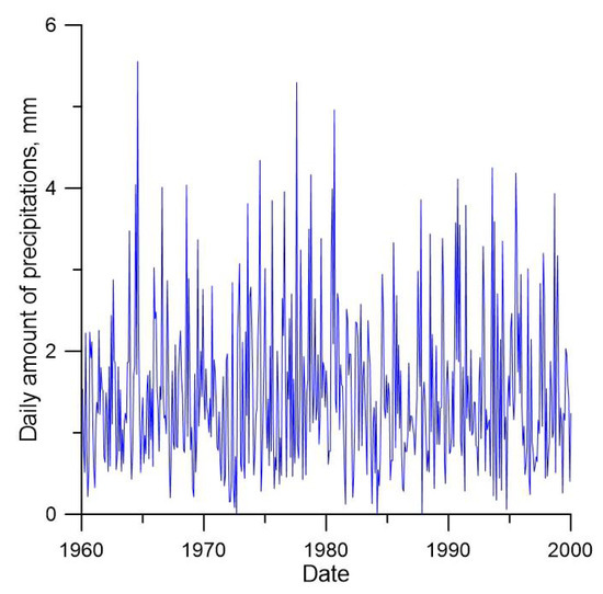
Figure 8. Atmospheric precipitations at pollution site after [13].

Only a part of precipitation moisture enters the groundwater [7,14]. A fraction of precipitation is lost by runoff and evapotranspiration. It depends on relief, type of soil and plant cover, and presence of asphalt covering and buildings. It can be seen in Figure 4a that the area covered by the asphaltic surface is not significant. Estimation of the fraction of atmospheric precipitations which enter the modeling domain is based on a simple model presented in [14]. According to this model, water infiltration rate (without evaporation) can be estimated as

$$w_I=\left\{\begin{array}{c}{w}_A,\hspace{1em}\mathrm{if}\hspace{0.33em}{w}_A\le w_{cr};\\ w_{cr}+{\alpha }_I\left(w_A-w_{cr}\right),\hspace{1em}\mathrm{if}\hspace{0.33em}{w}_A\ge w_{cr}.\end{array}\right.\hspace{0.33em}$$

(14)

$w_I$ is volume of infiltration which enters the underground medium per day through the unit open surface; $w_A$ is volume of precipitation moisture which enters the unit surface per day; $w_{cr}$ is critical rate of daily precipitations; ${\alpha }_I$ is a dimensionless coefficient.

According to recommended values from [14], parameters of the model in the considered case were specified as $w_{cr}$ = 37 mm and ${\alpha }_I$ = 0.88. Finally, an average value of $w_I$ was determined as

$$w_I^{av}=\frac{1}{N}{\displaystyle \sum _{n=1}^N{(w_I)}_n}$$

where $N$ is number of days of some time interval and ${\left(w_I\right)}_n$ is $w_I$ calculated from expression (14) for a day with number $n$. We considered a time interval of 30 years and obtained $w_I^{av}$ = 1.489 mm/day.

Taking into account evapotranspiration, $w_u$ can be determined from $w_I^{av}$ as

$$w_u=c_{et}{w}_I$$

where $c_{et}$ is a dimensionless coefficient. Climatic conditions of the Voronezh region correspond to $c_{et}$ = 0.3, and finally $w_u$ = 4.46 × 10⁻⁴ m/day.

$w_l$ characterizes groundwater inflow from the lower aquifer beneath the argillaceous layer A (Figure 4b). This value is equal to vertical component of Darcy’s velocity in the low-permeability layer between these aquifers. Hydraulic conductivity of upper Cretaceous clays at the considered site is approximately equal to 10⁻⁴ m/day, according to data from the enterprise “Hydrospetsgeologiya”. One can expect that argillaceous clay of the low-permeability layer is even less. We denote this value as $f_{\arg }$. The difference between hydraulic head in the lower aquifer and level of the groundwater in the upper aquifer is about 12 m. Thickness of the waterproof layer at the site is about 20 m (Figure 4b). Hence, we can estimate $w_l$ as

$$w_l\cong f_{\arg }\frac{\Delta H}{{\delta }_{\arg }}\le 6\times {10}^{-5} \mathrm{m}/\mathrm{day}$$

Since $w_l/w_u<<1$, $w_l$ can be neglected in (13).

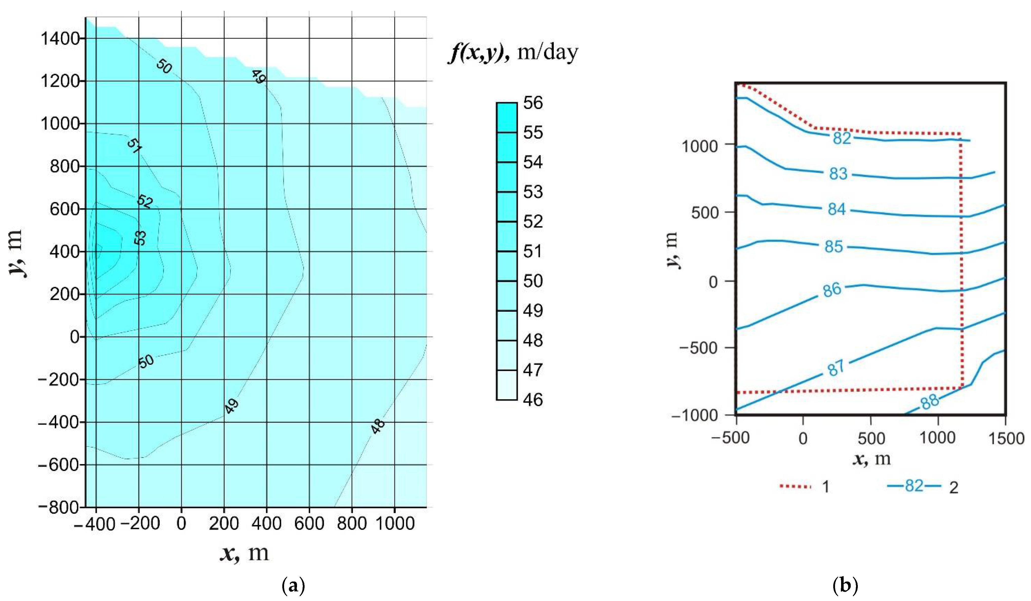
Subsequent procedure of calibration is absolutely the same, as in the case of the confined aquifer. Obtained distribution of water conductivity is shown in Figure 9. One can see that spatial heterogeneity of hydraulic conductivity is not significant to what corresponds to results of exploratory drilling of the aquifer.

Figure 9. Calibration of the model of groundwater flow at APP Novovoronezhskaya. (a) Distribution of hydraulic conductivity of the free aquifer; (b) water table elevation levels.

4. Conclusions

A characteristic feature of aquifers is elevated permeability in comparison with enclosing rocks. In a case of a pollution by liquid radioactive waste, aquifers represent a substantial hazard in view of elevated velocity of groundwater flow. Pollution can take place in both confined and free aquifers. An important part of input data for calculation of groundwater velocity in the polluted aquifers is spatial distribution of their permeability, which can be substantially heterogeneous. This can take place even at low permeability gradients due to significant dimensions of the domain. The only data for determination of such distribution consists of results of measurements in exploratory boreholes. However, drilling of the latter is a time consuming and expensive procedure. That is why the number of such measurements is usually limited. In addition to that, measurements are of different types (transmissibility and hydraulic head in confined aquifers and hydraulic conductivity and elevation of hydraulic head in free aquifers). We proposed a technique for determination of spatial distribution of transmissibility or hydraulic conductivity on the basis of measurements of all the types, simultaneously. The technique reduces the problem of the distribution determination to a search of a conditional minimum of a functional, with conditions in the form of equations in partial derivatives. The successful solution of the problem is demonstrated on examples of a confined aquifer (site of deep-injection disposal of liquid radioactive waste in the Krasnoyarsk region) and a free aquifer (site of radioactive pollution at the territory of atomic power plant Novovoronezhskaya) in Russia.

References

- Lovasic, Z. International Energy Atomic Agency (IAEA) Update on Spent Fuel Management Activities with Focus on Reprocessing. In Proceedings of the Waste Management Conference, Phoenix, AZ, USA, 24–28 February 2008; CD Version. p. 8042. [Google Scholar]
- Greene, C. Global Spent Fuel Overview; UXC: Roswell, GA, USA, 2020; Available online: www.uxc.com (accessed on 1 February 2021).
- Kochkin, B.T.; Malkovsky, V.I.; Yudintsev, S.V. Scientific Basis for Safety Assessment of Geological Isolation of Long-Lived Radioactive Waste; IGEM RAS: Moscow, Russia, 2017; 384p. (In Russian) [Google Scholar]
- Kopirin, A.A.; Karelin, A.I.; Karelin, V.A. Technology of Production and Reprocessing of Nuclear Fuel; Atomenergoizdat: Moscow, Russia, 2006; 576p. [Google Scholar]
- Rybal’chenko, A.I.; Pimenov, M.K.; Kostin, P.P.; Balukova, V.D.; Nosukhin, A.V.; Mikerin, E.I.; Egorov, N.N.; Kaimin, E.P.; Kosareva, I.M.; Kurochkin, V.M. Deep Injection Disposal of Liquid Radioactive Waste in Russia; Foley, M.G., Ballou, L.M.G., Eds.; Battelle Press: Columbus, ON, USA, 1998; 206p. [Google Scholar]
- Shchukin, A.P. Calculated-Theoretical and Experimental Studies of Patterns of Environment Pollution Due to Radionuclides Escape from a Repository of Liquid Radioactive Waste (on an Example of Atomic Power Plant Novovoronezhskaya). Ph.D. Thesis, All-Russian Research Institute for Nuclear Power Plants Operation, Moscow, Russia, 2007; 118p. (In Russian). [Google Scholar]
- De Marsily, G. Quantitative Hydrogeology; Academic Press: Cambridge, MA, USA, 1986; 440p. [Google Scholar]
- Scheibe, T.D.; Freyberg, D.L. Use of sedimentological information for geometric simulation. Water Resour. Res. 1995, 31, 3259–3270. [Google Scholar] [CrossRef]
- Zienkiewicz, O.C.; Morgan, K. Finite Elements and Approximation; John Wiley & Sons: Hoboken, NJ, USA, 1983; 328p. [Google Scholar]
- Becker, E.B.; Carey, G.F.; Oden, J.; Tinsley, J. Finite Elements. Englewood Cliffs; Prentice Hall: Hoboken, NJ, USA, 1981. [Google Scholar]
- Rice, J.R. Matrix Computation and Mathematical Software; McGraw-Hill: New York, NY, USA, 1981; 248p. [Google Scholar]
- Ravindran, A.; Reklaitis, G.V.; Ragsdell, K.M. Engineering Optimization: Methods and Applications, 2nd ed.; John Wiley & Sons: Hoboken, NJ, USA, 2006; 667p. [Google Scholar]
- Meteorological Observations. Available online: http://cliware.meteo.ru/inter/data.html (accessed on 1 February 2010).
- Anderson, M.G.; Burt, T.S. (Eds.) Hydrological Forecasting; John Wiley & Sons: Hoboken, NJ, USA, 1985. [Google Scholar]
Publisher’s Note: MDPI stays neutral with regard to jurisdictional claims in published maps and institutional affiliations. |
© 2022 by the author. Licensee MDPI, Basel, Switzerland. This article is an open access article distributed under the terms and conditions of the Creative Commons Attribution (CC BY) license (https://creativecommons.org/licenses/by/4.0/).