Study of Gas-to-Liquid Heat Pipe Heat Exchanger

Abstract

This study is focused on the study and development of a gas-to-liquid heat pipe heat exchanger (HPHE) based on numerical and experimental analysis. Stainless steel heat pipes were installed inside the heat exchanger in the form of three equilateral triangles, staggered into a hexagonal configuration to simulate the waste heat recovery from hot exhaust gas to a water flow. The first main aim of this study was focused on 3D design and numerical analysis, which were used to create and calculate the effect of similar input conditions on the overall system. The system was tested for the overall heat transfer by measuring the temperature change in both fluids. The heat transfer and overall average temperature were used to calculate the effectiveness of the system. In the second part of this study, a test of the waste heat recovery was undertaken with this setup, using water as the cooling fluid. The study was conducted with different input velocities and temperatures of waste hot air, controlled simultaneously by the input fan and air heater, whereas the cooling water was kept at a steady state of 30 °C and 0.0156 kg/s at the input. The hot air velocity was controlled by fans with different inlet air velocities of 0.3 m/s, 0.5 m/s, and 0.7 m/s. Moreover, the temperature of the air was changed from 150 °C to 250 °C with a step of 25 °C. The increase in temperature and the velocity of air was directly proportional to the amount of heat transferred from the air to the cooling water, and the effectiveness was also found to be inversely proportional to both of the varying input parameters. The numerical study showed a maximum increase of 12% in the heat transfer. The output temperatures of hot and cold fluids showed maximum increases of 7 K and 3 K, respectively. The numerical system with such input parameters can be evaluated further to predict the behavior of changes in the design and parameters.

1. Introduction

Heat exchangers are a very common device used for saving energy and they have been used for many years in various fields. The ability to transfer heat without the mixing of fluids is one of the most common traits of a heat exchanger. Heat pipes are passive heat transfer devices that use the latent heat of the internal working fluid to transfer heat faster due to the temperature difference. The heat exchanger works on both thermosyphons and heat pipes, which generally for low temperatures require a 5 °C difference in temperature for operation and specifically depend upon a hot fluid temperature for the startup of the heat pipe. Heat exchangers are generally sorted into two categories—regenerative or recuperative.

In the regenerative-type heat exchanger, the heat needs to be extracted from the hot section or heat needs to be provided to the cold section. In the recuperative-type heat exchanger, the fluids of different temperatures do not come in direct contact but are separated with a wall, and this is also generally known as the plate-type heat exchanger. Heat exchangers can also be further divided into categories according to fluid flow arrangements. Generally, the arrangements are co-current (hot and cold fluid flow in the same direction), countercurrent (hot and cold fluid flow in the reverse direction) and cross current (hot and cold fluid flow perpendicular to each other). Furthermore, another method of differentiation is based on the type of heat transfer, i.e., gas-to-gas, gas-to-liquid and liquid-to-liquid.

The type of heat exchanger discussed in this report is the recuperative-type counterflow gas-to-liquid-type heat exchanger [1]. The advantages of the use of a heat pipe varies with different applications and requirements, although in conditions where direct contact is not required and the heat transfer needs to be fast, the heat pipe heat exchanger is a valid and easy choice. Energy conservation is also a very important issue in the modern world and the industrial revolution made it a necessity. Most of the waste in modern industries are waste gases and that waste is also a major factor in decreasing the efficiency of systems. There are three categories of waste gases—high temperature (above 650 °C), medium temperature (250–650 °C) and low temperature (below 250 °C) [2]. Thus, heat exchangers use the waste energy and increase the overall efficiency of the system and decrease environmental pollution.

Several studies have been conducted on heat pipe heat exchanger (HPHE) development. The design and classification were presented by Faghri et al. [1] and Shabgard et al. [3] described the advantages and various applications of heat pipe heat exchangers. The various applications of heat pipe heat exchangers provide different challenges and their design has evolved for different situations. Heat pipe heat exchangers have been used in various applications, such as the heating and cooling of devices, air conditioning, waste heat recovery from combustion gases, data center cooling, power plant dry cooling towers, steam condensers, latent thermal energy storage for solar power generation, and CPU cooling in laptop computers.

Further works conducted by Lukitobudi et al. [4], Martinez et al. [5] and Geoola et al. [6] presented further studies of different heat pipe heat exchangers. The study conducted by Azad in 1984 reported one of the oldest heat pipe heat exchanger, used for cooling with gravity-assisted heat pipes. The author further combined fins with the heat pipes and also used different spacings of tubes to obtain the desired behavior. That study examined the effect of fins per area as well as the effectiveness improvements obtained through increasing the area of the evaporator and using different spacing in the tubes. The overall effectiveness analysis, performed using the NTU method, showed the results to be affected by the area of the fins. Lukitobudi analyzed the use of a thermosyphon heat exchanger design for a bakery, which is a very common and very useful application. The use-case was under 300 °C; thus, it was a medium-temperature operation. The author used Freon 22 as the fluid in the thermosyphon, heat transfer rates were achieved between 4 to 20 kW and the heat exchanger was reliable for being in use for over several years. In another study, Srimuang et al. [7] discussed the effects of a heat exchanger as a method of saving the waste heat from various applications. Their report summarized the heat pipe and thermosyphon, as well as the oscillating thermosyphon used in the heat exchanger in a waste heat recovery system and compared the data gathered by others in terms of effectiveness. The study carried out by Bing et al. [8] examined the functioning of a heat pipe heat exchanger with different input conditions and calculated the heat recovery achieved using cold fluid at the cold end. The study was conducted using FLUENT software (Ansys, Canonsburg, PA, USA) and the input velocity of air is taken to range from 0.02 m/s to 0.12 m/s and the recovered heat was calculated in watts. The study showed that the heat transfer can be calculated based on the temperature of the hot air. The higher velocity reduced the heat recovery and the best heat recovery by the cold fluid was observed at an air velocity of 0.04 m/s inlet. The dimensions of this study model were not very large; thus, it can be considered a small-scale application. Furthermore, Rashidian et al. [9] made a similar model and tested the waste heat recovery of a heat pipe heat exchanger. This study was similar but was carried out using MATLAB software and and the numerical analysis was based entirely on the analytical calculations and the equation-based method. The authors designed a 2D working model with different working conditions but the results were basically based on the driving equation which was developed by Saber et al. [10] also used FLUENT for their design but the input conditions were also specific to the user’s case scenario. The results of that study were also analyzed according to the performance of a heat exchanger without losses.

Experimental and theoretical studies by Aliabadi et al. [11] investigated the effects of the heat capacity ratios of high- and low-temperature fluid streams, the inlet hot air temperature and the mass flow rate or the inlet hot air velocity on the thermal performance of a gas–liquid thermosyphon heat pipe heat exchanger. An air-to-water heat exchanger equipped with wickless heat pipes was investigated experimentally for a range of inlet flow conditions on the evaporator side by Ramos et al. [12]. Although the heat transfer rate increased with increasing mass flow rates, the effectiveness of the heat exchanger exhibited a constant downward trend, a result of the hot air not having enough time to transfer its heat to the pipes. CFD modeling and numerical calculations were demonstrated by Ramos et al. [13] to predict the thermal performance of a cross-flow wickless heat pipe-based heat exchanger. The heat pipes were considered as solid devices with a known thermal conductivity, which was estimated based on experiments.

The aim of this study was to create an experimental design for a gas-to-liquid heat pipe heat exchanger and study its performance with different input conditions. This paper presents the testing of the heat pipe heat exchanger with a new heat pipe made from a combination of different materials chosen for various parts. The novel design of the heat pipe was devised using composite materials for its construction, consisting of stainless steel for the pipe and copper mesh inside. The copper mesh provides the optimum capillary and heat transfer, whereas the stainless-steel exterior protects the pipe from erosion and corrosion from different elements. An experimental study was conducted to ensure the workability of this device for waste heat management in small industries, in which reliability in harsh conditions becomes vital over time. The study also included a numerical study, conducted using CFD software to create a similar problem to that in the experiment in order to quantify and compare the results from the experiments. For the analysis of this kind of heat transfer device, it would be necessary to design, build and conduct tests, which may lead to high costs and the wastage of time and human resources. The goal of the comparison of both studies is to show that the numerical changes are comparable with real-world experiments. The numerical analysis was carried out with as close an approximation as possible with the experimental studies in order to predict the system’s behavior in the real world. This will provide us with a better base to conduct further analyses using numerical analysis software and thus saving resources.

2. Numerical Study of HPHE

The numerical analysis was developed for a small heat exchanger with water cooling. The design of the analysis was conducted based on the experiment proposed for the real-world testing. We attempted to mimic the experimental conditions in the numerical analysis by using different boundary conditions. Numerical analysis was carried out using ANSYS-FLUENT CFD software. We made some assumptions, which are mentioned below, for the numerical analysis.

• The heat and velocity in the input of both fluids was kept steady, and could be assumed to be a steady heat input for the heat pipes.
• The materials were selected in the software with all standard values of properties, represented in the FLUENT database. The heat pipe material created for the analysis thus may not show the exact behavior of the heat pipes as it does not undergo a phase change.
• Heat losses for the outside shell depended upon the material and were assumed to be steady for the entire process.
• There was no heat loss between the heat transfers from heat pipes between both fluids, and all the heat transfers between both fluids were carried out by heat pipes only.
• The velocity profile and temperature of the fluid were symmetrical on only the input surfaces.
• The analysis used a controlled environment at a steady temperature which did not have any effect on the airflow or water flow sections.

2.1. Design for Numerical Analysis

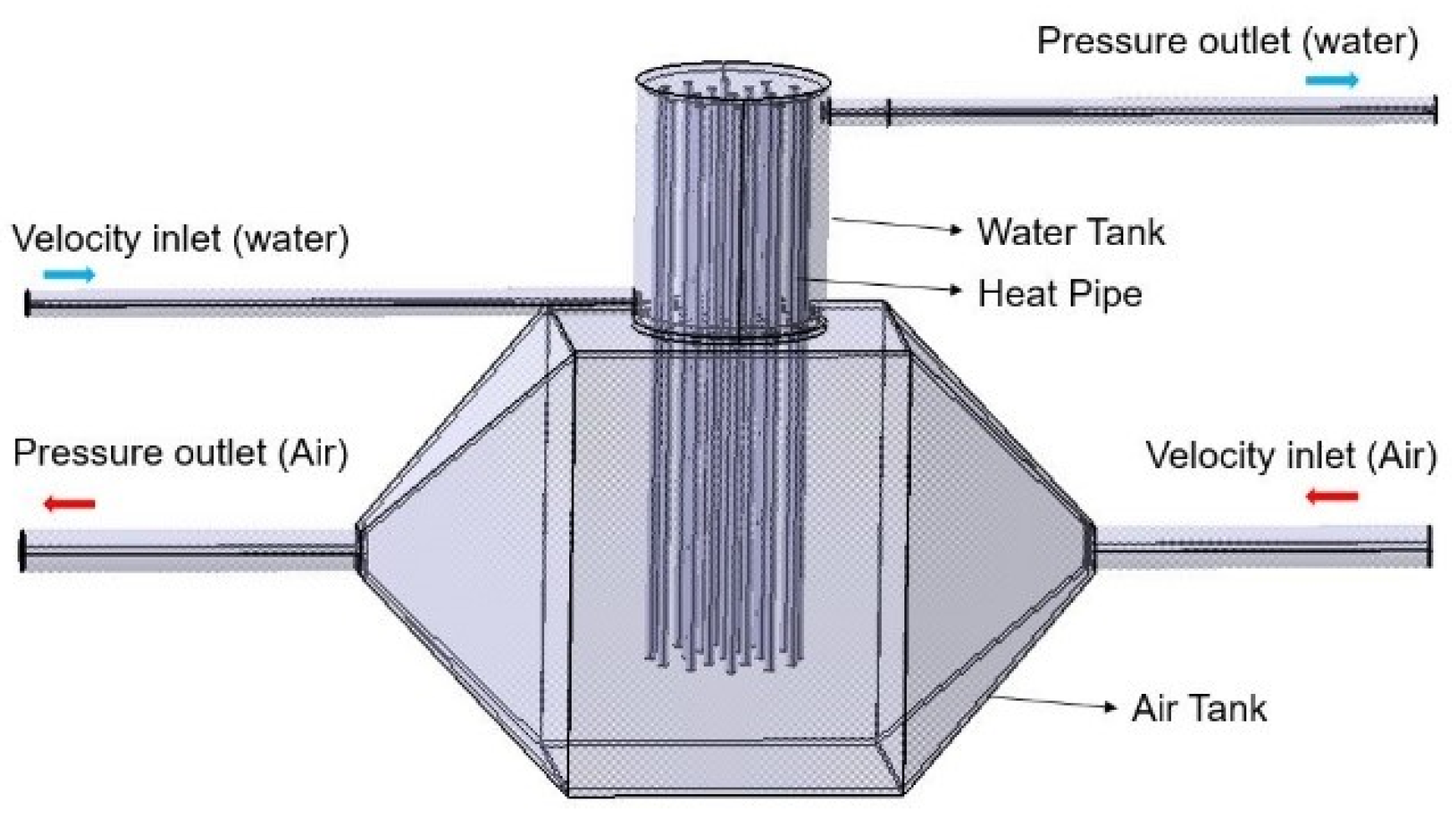
The design of the HPHE was created using the design software SOLIDWORKS 16.0 (Velezi-Villacoubre, France) and the dimensions were based on the heat pipe length. The design made using this software is shown in Figure 1. The design includes the heat pipes, which are constructed like a solid pipe in the software and which were given the same thermal properties as a heat pipe according to the material properties in the FLUENT software. The pipes thus behave very similarly to an actual heat pipe in the heat transfer analysis and give a similar result. The design of the pipe was made to be similar to a single cylinder with the properties changed to mimic a heat pipe, which was also arranged in a set of 19 pipes, using the same method as that of the experimental design.

In the design process, we did not have a controlled environment like the room in which the experiments were performed. Therefore, the design was enclosed in an outer boundary which created a controllable room in which the air was kept at room temperature (25 °C). The outer shell was 600 mm long, 400 tall and 280 mm wide. This entire volume is enough to cover the components and to cause no change in the outflow of water or air.

2.2. Numerical Modeling

For the numerical modeling and analysis, the governing equations were based on the K epsilon turbulence and transport models. The overall behavior of the fluid flow and turbulence change was based on the physical evaluation of the basic equation representing and expanding the continuity equations. The time-averaged continuity equation is represented by Equation (1).

$$\frac{\partial {\overline{u}}_i}{\partial x_i}=0$$

(1)

The time-averaged momentum equation is presented in Equation (2)

$$\rho \overline{u_j}\frac{\partial {\overline{u}}_i}{\partial x_j}=\rho \overline{f_i}+\frac{\partial }{\partial x_j} \left[-\overline{p}{\partial }_{ij}+2\mu \overline{S_{ij}}-\rho \overline{u_i^{\prime }}\overline{u_j^{\prime }}\right]$$

(2)

In Equation (2), the term $\overline{S_{ij}}$ represents the strain tenson. The strain tension is given by the formula in Equation (3)

$$\overline{S_{ij}}=\frac{1}{2} \left(\frac{\partial \overline{u_i}}{\partial \overline{x_j}}+\frac{\partial \overline{u_j}}{\partial \overline{x_i}}\right)$$

(3)

The time-averaged energy equation is given by Equation (4)

$$U_i\frac{\partial \overline{T}}{\partial x_i}=\frac{\partial }{\partial x_i}\left(\alpha \frac{\partial \overline{T}}{\partial x_i}-\overline{u_i^{\prime }}\overline{T^{\prime }}\right)+S$$

(4)

In terms of a direct analogy to the turbulent momentum equation for transport in energy, turbulent heat or mass transport is often assumed to be in direct correlation with the gradient of transport quantity. Equation (5) represents the mentioned gradient as follows:

$$-\overline{u_i^{\prime }}\overline{T^{\prime }}={\alpha }_t\frac{\partial \overline{T}}{\partial x_i}$$

(5)

In Equation (5) ${\alpha }_t$ is the turbulent diffusivity of heat and mass. Similarly to eddy viscosity, ${\alpha }_t$ is dependent upon the state of turbulence despite not being a property of the fluid. According to the Reynolds analogy between heat and mass, we can obtain Equation (6).

$${\alpha }_t=\frac{v_t}{{\sigma }_t}$$

(6)

Here, the quantity ${\sigma }_t$ is called the turbulent Prandtl or Schmidt number.

The equation for turbulent kinetic energy (k) and its dissipation rate ($\epsilon$) is given by Equations (7) and (8).

$$U_i\frac{\partial k}{\partial x_i}=\frac{\partial }{\partial x_i}\left(\frac{v_t}{{\sigma }_k}\frac{\partial k}{\partial x_i}\right)+v_t\left(\frac{\partial U_i}{\partial x_j}+\frac{\partial U_j}{\partial x_i}\right)\frac{\partial U_j}{\partial x_j}-\epsilon$$

(7)

$$U_i\frac{\partial \epsilon }{\partial x_i}=\frac{\partial }{\partial x_i}\left(\frac{v_i}{{\sigma }_{\epsilon }}\frac{\partial \epsilon }{\partial x_i}\right)+C_{1\epsilon }\frac{\epsilon }{k}p-C_{2\epsilon }\frac{{\epsilon }^2}{k}$$

(8)

where p is the generation of k and is represented by Equation (9)

$$P=v_t\left(\frac{\partial U_i}{\partial x_j}+\frac{\partial U_j}{\partial x_i}\right)\frac{\partial U_i}{\partial x_j}$$

(9)

Furthermore, the turbulent viscosity is related to k and $\epsilon$ by the expression in Equation (10)

$$v_t=C_{\mu }\frac{k^2}{\epsilon }$$

(10)

The coefficients $C_{\mu }$, $C_{1\epsilon }$, $C_{2\epsilon }$, ${\sigma }_k$ and ${\sigma }_{\epsilon }$ are constants which have the following derived values.

$$\begin{gathered} C_{\mu }=0.09 \\ {C}_{1\epsilon }=1.44 \\ {C}_{2\epsilon }=1.92 \\ {\sigma }_k=1.0 \\ {\sigma }_{\epsilon }=1.3 \end{gathered}$$

2.3. Mesh and Boundary Conditions

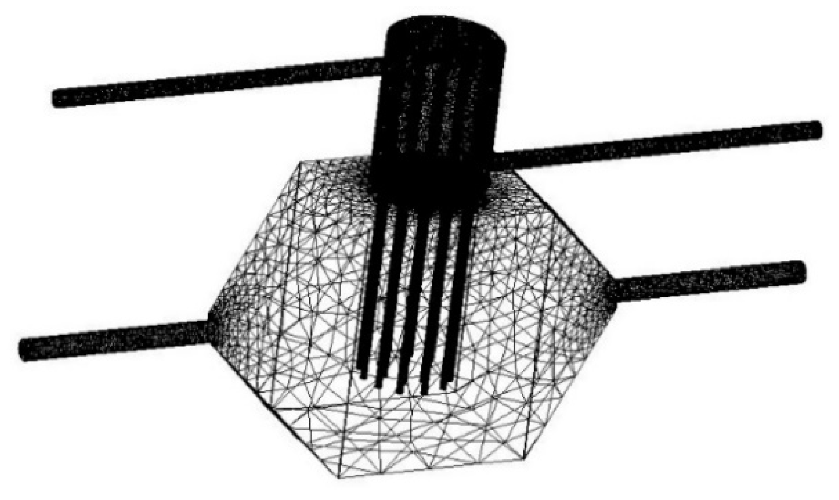
The mesh is a very important component for the numerical analysis. In our case, we performed the meshing with a given size for each different component. The meshing size and inflation of faces for smaller pipes will ensure a better mesh with a high quality. Figure 2 shows the meshing performed for our case. The smaller elements and important elements such as heat pipes had a very fine mesh. The outside boundary worked at a constant temperature and thus did not require very fine mesh. According to the meshing tool, the total number of elements for this mesh was 2.8 million, with the orthogonal quality of 0.9960. The design included a finer mesh for the water section because the size of the container and the higher thermal conductivity of water made the heat transfer higher per mesh element.

In order to ensure that the solution was independent of mesh sizes, we created different sizings for each case and ran the tests, which yielded the data presented in

Table 1. Mesh independence study.

Case Number	Mesh Elements	Orthogonal Quality of Mesh	Average Air Temperature	Average Water Temperature
Case 1	8364251	0.9835	77.146 °C	32.92 °C
Case 2	28494887	0.9960	77.157 °C	32.92 °C
Case 3	45621553	0.9958	77.157 °C	32.92 °C
Case 4	103212641	0.9945	77.157 °C	32.92 °C

. According to Table 1, the mesh changes showed a very small change in the quality of the mesh and the average temperature of the air and water sections. For the heat pipes, we kept the fine-quality mesh because of its smaller size. For an air input temperature of 150 °C and a water input temperature of 30 °C, the result for the validation cases are shown in Figure 3. The difference in the overall temperature with different mesh sizes cannot be differentiated visually. The maximum difference between different cases was 0.2 K for the air outlet, whereas the water side remained at the same temperature. We were able to choose a mesh number when the output temperature stopped changing with the mesh; thus, the calculation process did not become time consuming. Hence, the mesh with 2.8 million elements was chosen for the rest of the solutions because there was no considerable difference between this and meshes with higher numbers of elements.

2.4. Input Parameters for Numerical Analysis

For the input of the numerical analysis, the material of the tank was designated as steel in the software’s pre-defined material section. The fluid for each section was designated as water and air. To make heat pipes, we defined a material which has a very high thermal conductivity (5000 W/(mK)), like that of heat pipes. The input velocity of air was kept at 0.3 m/s, 0.5 m/s and 0.7 m/s, whereas the water mass flow rate was kept constant at 0.0156 kg/s. The temperatures were varied similarly for air, from 150 °C to 250 °C with 25 °C variations, whereas water is kept at a constant temperature of 30 °C. The flow time was designated as 100 s during the numerical analysis in order to achieve a steady state of flow.

3. Experimental Study of HPHE

In this study, we aimed to analyze the capacity of heat recovery and performance targets for the heat pipe heat exchanger of a relatively small size. The experimental parameters were set based on the numerical analysis and the test setup requirements. This experiment was focused on low-temperature exhaust gas (below 250 °C) discharged from industrial waste heat or other applications in which energy conservation is important.

3.1. Heat Pipe Specifications

The heat pipe heat exchanger was designed to work at temperatures below 250 °C. Therefore, water could be chosen as the cooling liquid due to its universal availability and high thermal conductivity and heat capacity. The use of water would allow a smaller cooling section as the water would acquire more heat from the waste gas. Furthermore, water was chosen as the working fluid inside the heat pipes due to its adequate performance in medium-temperature situations. The waste gases mostly consisted of hydrogen sulfide, sulfuric acid, dust and other pollutants and particles. Therefore, the contact surface of the heat pipe can be easily corroded. The heat pipes were thus made from 316 L stainless steel with a smooth surface. The dimensions of the heat pipe were 6.2 mm outer diameter, 0.5 mm wall thickness and 300 mm in total length. The capillary structure was mounted on the inner wall of the container with a layer of 200-element mesh made with cooper. The filling volume of the working fluid was injected into the fluid corresponding to the pore size and capillary structure, which was in the range of 1.4–1.5 g. The metal container was filled with working fluid and then vacuumed to 1 × 10⁻¹ torr, followed by degassing of the pipe and clamping two times to eliminate non-condensable gases.

3.2. Arrangement and Setup of Equipment

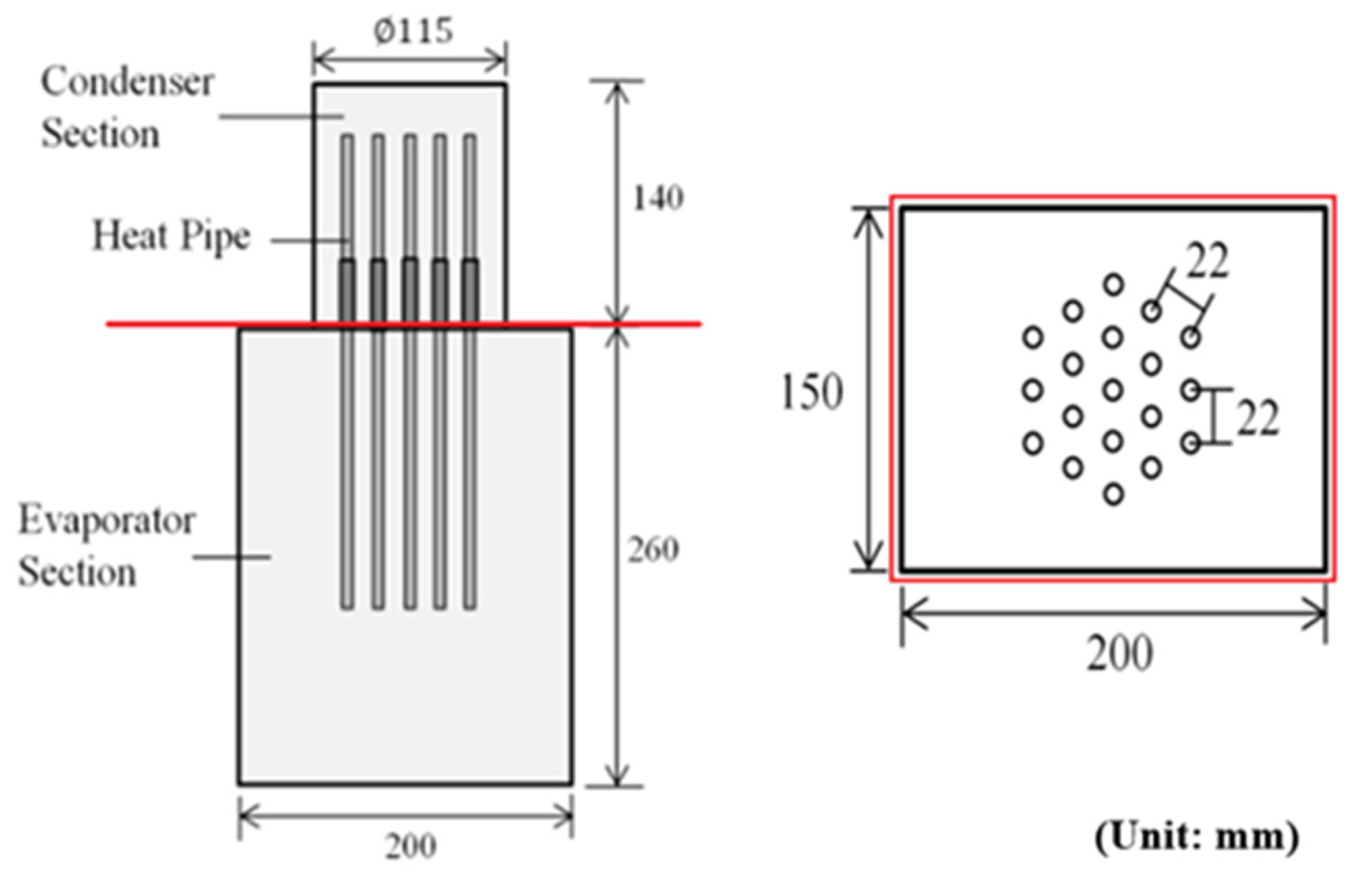
In this study, the gas–liquid heat pipe heat exchanger was tested under different conditions. The bottom tank, which provides hot air for heating the heat pipes, is known as the evaporation section. The top end provides cooling water and is known as the condensation section. The evaporator end of the device is shaped as a cuboid with a length of 200 mm, a width of 150 mm and a height of 260 mm. The condenser end of the device is a cylinder with an outer diameter of 115 mm and a height of 140 mm. Both sections are made out of steel with a thickness of 4 mm. A total of 19 heat pipes can be installed inside the heat exchanger in an orientation consisting of three equilateral triangles staggered into a hexagonal shape with the center being a single pipe. The arrangement and spacing are shown in Figure 4.

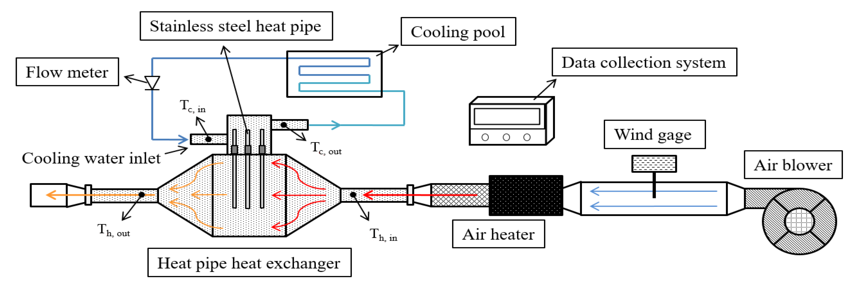
The test platform consisted of a blower, air heating machine, anemometer, heat pipe heat exchanger, temperature acquisition system, flow meter and temperature-controlled water tank. The air was blown into a stainless-steel container with an inner diameter of 83.5 mm via a blower, and then it flowed through the blower section. After it was heated by an air heater, the blower transferred the hot air into the right side (Th, in) of the heat exchanger. Then, the air was transferred to the heat pipes and hot air exited from the left side (Th, out) of the heat exchanger. On the other hand, the water flowed through the condensation end, starting from the left side (Tc, in), into the cooling water cycle to reduce the temperature and was then taken out on the right side (Tc, out). The water flow rate was controlled using a flow meter, and an anemometer was used to measure the airflow rate in the pipe.

In the experiment, the temperature of the fluid was read using a thermocouple wire connected to the temperature measurement module and recorded in the data acquisition system. The main temperature measurement points were located at the points where the hot gas and cooling water passed in and out of the heat exchanger, respectively. The heat exchanger was covered with cotton padding insulation to avoid heat loss and air convection interference. The layout of the experimental setup is shown in Figure 5.

The specifications of the equipment used for testing and mentioned in Figure 5 were as follows.

• Air blower and air heater—the air heater and blower were designed by the same company in conjunction. The air blower was used to control the air inlet velocity in terms of the capacity of the blower and the air heater was used to maintain a specific temperature of inlet air. The air blower used in the test was the SILENCE blower from the LEISTER company in Germany and the model used was 9 G-32. The air heater tested was an LHS Classic 61 L hot air blower from the LEISTER company in Germany. It had a 3-phase 230 V voltage with a maximum input power of 10 kW, a minimum air volume of 1000–1800 L/min and a maximum achievable temperature of 650 °C. It was equipped with a temperature control box to control and display temperature changes to avoid overheating.
• Anemometer—the anemometer was used to measure the velocity of the air let in to the heat exchanger. It was installed in the air inlet part of the heat exchanger. The equipment used the hot-wire wind speed transmitter from Yitian Technology, New Taipei city, Taiwan and its model number was FTS34. The minimum wind speed measurement range was 0.2 m/s, with a wind speed accuracy of ±2%. Meanwhile, the thermal sensitivity in terms of the temperature was 0.1%/°C, and the protection level was IP54.
• Temperature measurement module—the temperature was measured with the help of a FBs-TC6 thermocouple temperature measurement module from FATEK’s FBs-PLC series. The measurement module was capable of being connected to six channels with variable temperature sensor types J, K, T, E, R, S, B and N. The resolution was 0.1 °C and the accuracy was ±(1% + 1 °C). There was a built-in contact compensation and temperature sensing wire disconnection detection circuit. In this study, we used a K-Type thermocouple for measurements.
• Thermostatic water cooler and tank—for the water or condensation end of the experiment, we used a P-50 low-temperature circulating water tank from Yifeng Instruments, New Taipei city, Taiwan. The temperature control range was 0–90 °C, with a control accuracy of ±0.5 °C and a maximum flow rate of 9 L/min.
• Flow meter—a flow meter was placed in the water-cooling loop to measure the water inlet mass flow rate. The device used was a general industry flow meter with a minimum printed reading of 0.05 L/min. The device also had a turn off valve, which also controlled the flow.

3.3. Method and Parameters of the Experiment

All the parameters were set for the test using the control panel, and then the temperature changes were observed and recorded during the experiment. First, the blower was set at a constant speed to fix the hot air mass flow rate. Secondly, the hot air temperature for input into heat exchanger was maintained around 150 °C. After the fluid temperature reached a steady state, the tests were changed for different input temperatures from 175 °C to 250 °C, with a 25 °C variation. In this test, the outflow was kept at a steady state, with the temperatures not changing more than ±1 °C.

Table 2. Input parameters for the experiment.

Controlled Parameters
Heat pipe specifications	Metal container material: SS316 L Outside diameter of heat pipe: 6.2 mm Wall thickness of heat pipe: 0.5 mmTotal length of heat pipe: 300 mm
Length of evaporator section and condenser section of heat pipe (mm)	Evaporator section 196 Condenser section 100
Number of heat pipes	19
Temperature of cooling water at inlet (°C)	30
Mass flow rate of cooling water at inlet (kg/s)	0.0156
Variable Parameters
Temperature of heating water at inlet (°C)	150, 175, 200, 225, 250
Inlet velocity of heating air (m/s) (The capacity of the blower as a percentage)	0.3 m/s (20%) 0.5 m/s (30%) 0.7 m/s (40%)

presents the input parameters for the experiment. To calculate the performance of a heat exchanger, it is usually analyzed in terms of the effectiveness (ε) of the process. Effectiveness (ε) was defined as the ratio of the actual heat transfer quantity q (W) of the heat exchanger to the maximum possible ideal heat transfer quantity q_max (W). It can be defined as follows:

$$\epsilon =\frac{q}{q_{max}}$$

(11)

The actual heat transfer quntity q is expressed as the exothermic quantity of hot fluids q_h or the heat absorption quantity of cold fluids q_c, which is calculated as:

$$q_h=m_h{C}_{p,h}\left(T_{h,in}-T_{h,in}\right)=C_h\left(T_{h,in}-T_{h,out}\right)$$

(12)

$$q_c=m_c{C}_{p,c}\left(T_{c,out}-T_{c,in}\right)=C_c\left(T_{c,out}-T_{c,in}\right)$$

(13)

The maximum possible ideal formula of the heat transfer quantity is as follows:

$$q_{max}=C_{min}\left(T_{h,in}-T_{c,in}\right)$$

(14)

In the above formulas, it was found that C_min was the smaller number between the heat capacity of hot fluids (C_h) and cold fluids (C_c). The heat capacity C was defined as the product of the fluid mass flow rate ṁ and the specific heat c_p. Therefore, validity can be ordered again using the formulas of Equations (12)–(14), following the works of Incropera et al. [14] and Kays et al. [15]:

$$\epsilon =\frac{C_h\left(T_{h,in}-T_{h,out}\right)}{C_{min}\left(T_{h,in}-T_{c,in}\right)} \mathrm{if} C_h>C_c$$

(15)

$$\epsilon =\frac{C_c\left(T_{h,out}-T_{h,in}\right)}{C_{min}\left(T_{h,in}-T_{c,in}\right)} \mathrm{if} C_h>C_c$$

(16)

Equations (15) and (16) represent the effectiveness of the system with different kinds of fluid-to-fluid heat transfer, depending on their heat capacity. The experiment involved errors due to instruments and human factors; thus, it was necessary to carry out uncertainty analysis. The factors that could cause experimental errors in this study were the fluid mass flow rate and temperature. All of these experimental errors will lead to calculation errors for the quantity of heat transfer and validation. The results regarding validity and uncertainty can be expressed according to Equation (17).

$$w_{\epsilon }={\left[{\left(\frac{\partial \epsilon }{\partial {\dot{m}}_h}{w}_{{\dot{m}}_h}\right)}^2+{\left(\frac{\partial \epsilon }{\partial {\dot{m}}_c}{w}_{{\dot{m}}_c}\right)}^2+{\left(\frac{\partial \epsilon }{\partial \mathsf{\Delta }{T}_{in}}{w}_{\Delta T_{in}}\right)}^2+\left(\frac{\partial \epsilon }{\partial \mathsf{\Delta }{T}_c}{w}_{\Delta T_c}\right)\right]}^{\raisebox{1ex}{$1$}\!\left/ \!\raisebox{-1ex}{$2$}\right.}$$

(17)

In this study, the validity was assumed to be a function ε, which contains several variables (${\dot{m}}_h$, ${\dot{m}}_c$, ∆T_in, ∆T_c), and all of these variables had an indeterminate value ($w_{{\dot{m}}_h}$, $w_{{\dot{m}}_c}, w_{\mathsf{\Delta }{T}_{in}}, w_{\mathsf{\Delta }{T}_c}$), which indicated the experimental errors. Through the experimental uncertainty analysis, we found that the experimental measurement error for the hot gas mass flow rate was ±2%, that of the cooling water mass flow rate was ±1% and that of temperature was ±1 °C, respectively.

3.4. Results of Experiments

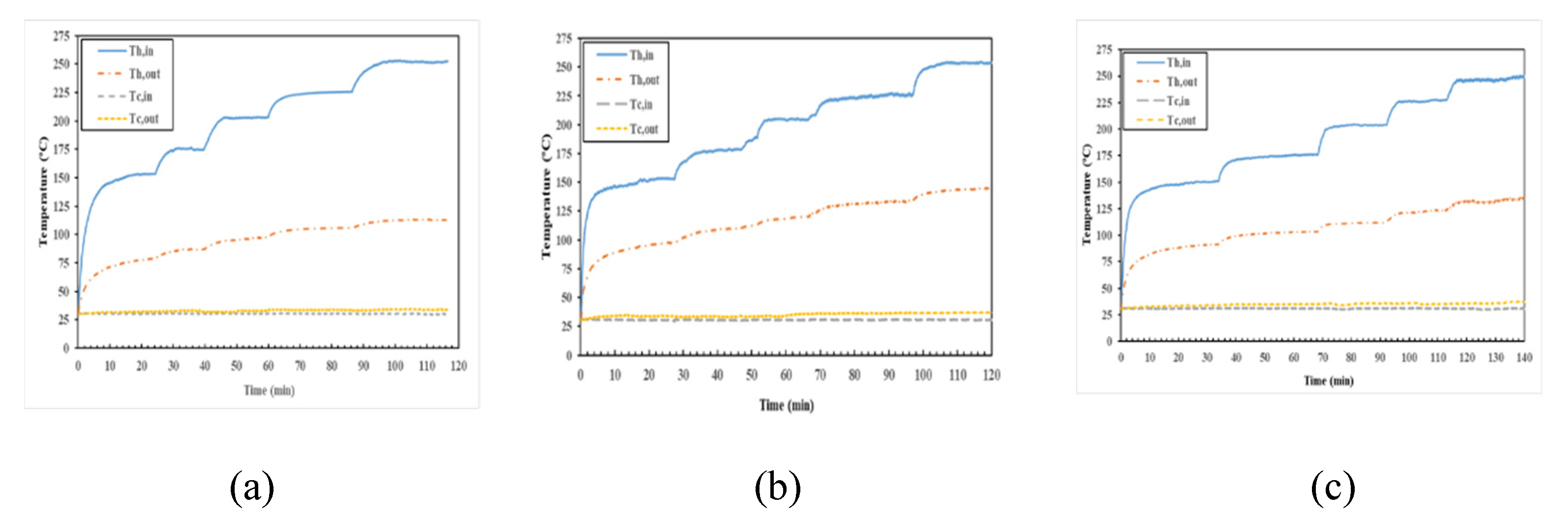
In the experiments, hot air at the hot end of the heat exchanger or the evaporation end of the heat pipe was changed to 150, 175, 200, 225 and 250 °C at different inlet air velocities of 0.3, 0.5 and 0.7 m/s, respectively. At the cooling end, the inlet water temperature of 30 °C and the mass flow rate of 0.0156 kg/s were maintained. The data were collected using four thermocouple wires, which were used to measure the temperature change of the fluid. Furthermore, the steady-state temperature data were collected to analyze the temperature change of the fluid. Figure 6a–c shows the temperature changes of the fluid over time. For each case, the hot air velocity was fixed at 0.3 m/s, 0.5 m/s and 0.7 m/s simultaneously and cooling water was fixed with a constant inlet temperature and mass flow rate. The output temperature gradually increased with inlet air temperature from 150 °C to 250 °C, which is shown in Figure 6 with steps. The results show that the inlet temperatures of the hot air and cooling water were increasing gradually. The results revealed that when the inlet velocity of hot air increased, the outlet temperature of the hot air and the difference between the inlet and outlet temperature decreased. The outlet temperature of water changed gradually as the inlet water temperature remained at 30 °C.

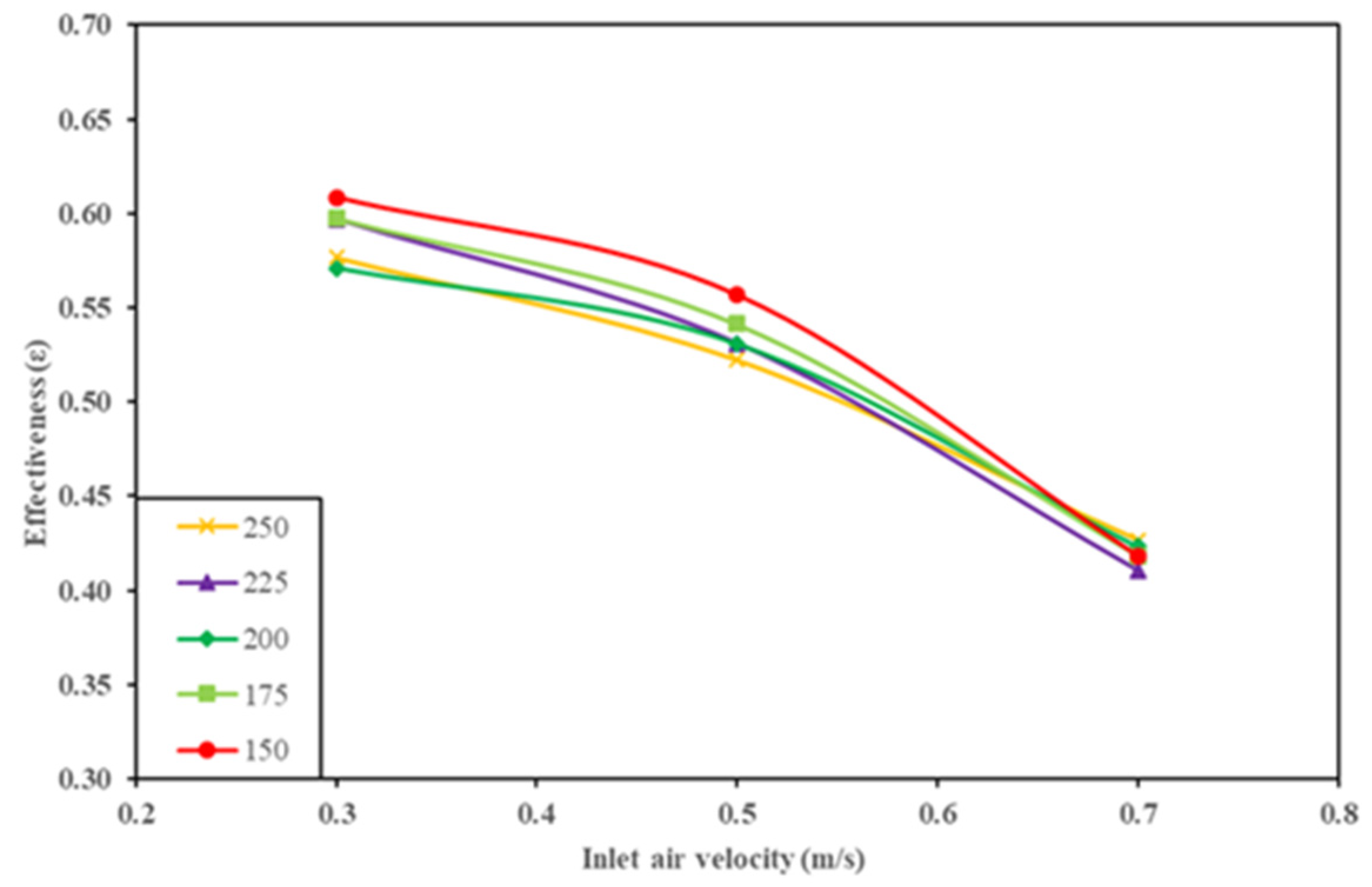
The results indicated that when the inlet velocity of hot air increased, the heat transfer per unit area increased accordingly. The overall increase in input heat from the hot fluid increased the cold fluid outlet temperature as well. The effect of the input air velocity and input air temperature can be shown regarding to effectiveness. The effectiveness is an important factor relating to the heat exchanger’s heat transfer ability. Figure 7 presents the effect of the hot air inlet velocity change in terms of effectiveness. Based on the experimental results, we found that the hot air inlet velocity rate was proportionally related to the resultant effectiveness. At lower hot air inlet temperatures, the effectiveness was higher in general, and with the increase in inlet air velocity the effectiveness decreased for all different inlet temperatures. The effectiveness showed that the desired input conditions included a lower inlet air velocity and a lower inlet air temperature. The maximum effectiveness of 0.609 was obtained when the inlet air velocity was 0.3 m/s and the inlet temperature was 150 °C. The lowest effectiveness of 0.410 was obtained when the inlet air velocity was 0.7 m/s and the inlet temperature was 225 °C.

4. Result and Discussion

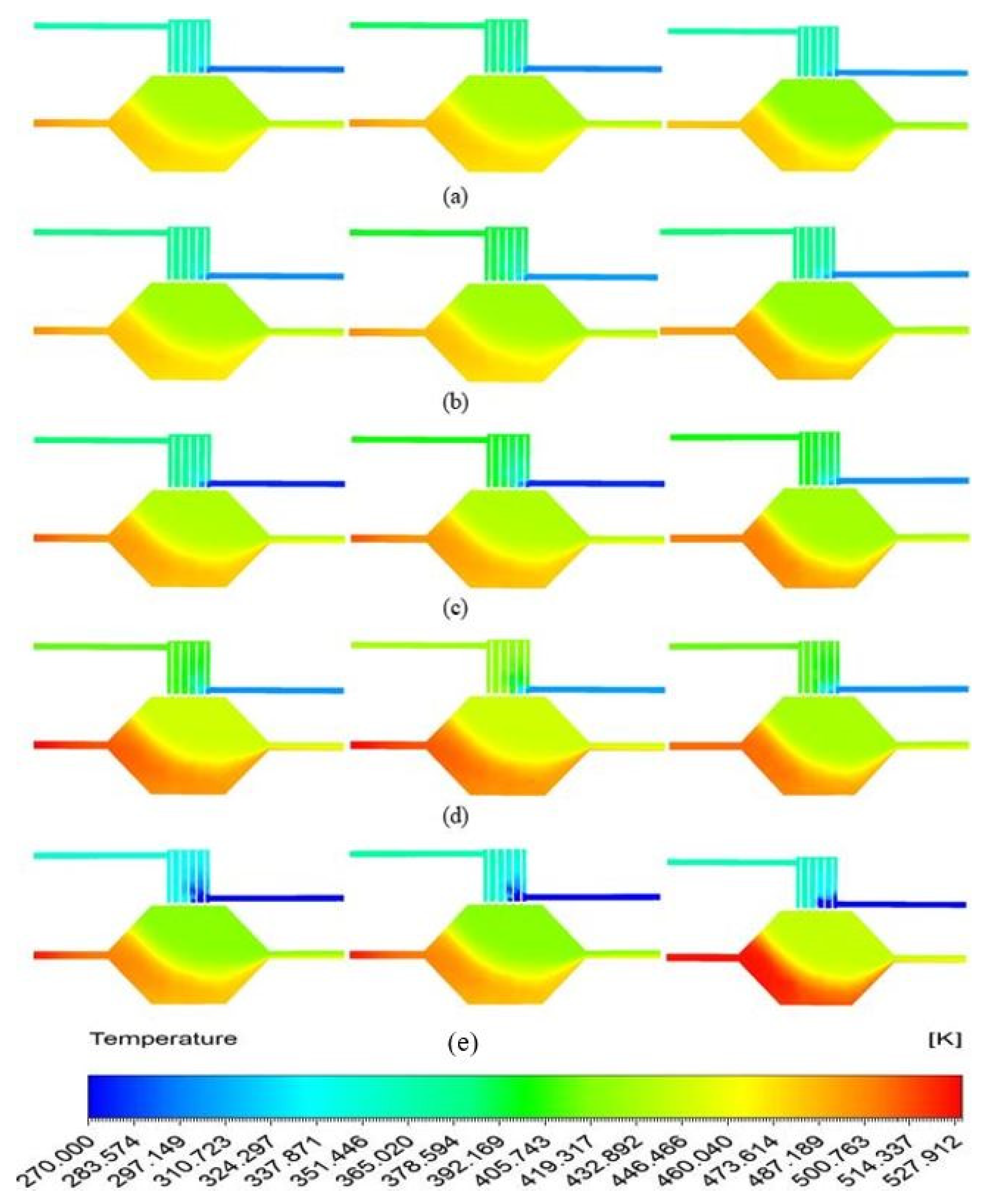
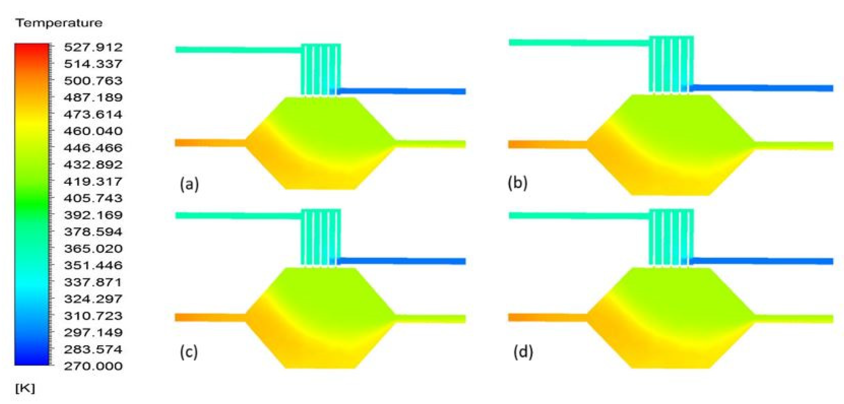
Here, we discuss the results of the output comparison of both the numerical and experimental analysis. For the numerical analysis, the temperature output was the most important section, as that was used to calculate the overall heat transfer and effectiveness. The average temperature output of the numerical analysis is shown in Figure 8, with different temperature scales. By observing the average temperature throughout the process, we can determine the effects of the velocity of air, as well as temperature, in relation to the overall heat transfer capacity. The temperature of the cooling water with the surroundings was affected when the air temperature increased, as the enclosure was made out of steel and the system was also given boundary conditions to replicate a closed environment. The closed environment also accounts for the heat loss that occurred during the process, which was not observed in the real-life scenario.The numerical analysis was conducted for the purpose of a comparison with a heat pipe heat exchanger in a controlled situation, but it would be helpful to develop the heat exchanger further. The amount of heat transfer or loss may not accurately reflect the real-life use case. Instead, the close output values will provide an indication for the further development of the design and development of the entire system. The comparison of the results could be carried out in this study by focusing on the overall temperature at the inflow and outflow of both fluids, as well as the heat transfer of both the evaporator and condenser sections.

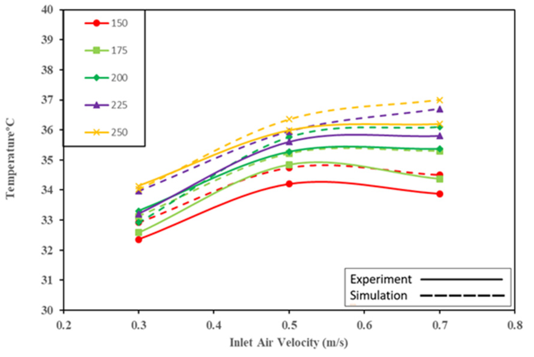
The results of the experimental and simulated systems had the same number of outputs, which can be divided into five different sections based on the different input temperatures of air, varying from 150 °C to 250 °C. The velocity of the air input was the same for both experiments and simulations; thus there was a total of 15 results for each analysis. In Figure 9 the results are represented with a solid line for experiments and a dotted line for the numerical analysis. The inlet temperature was dependent upon the blower and air heater for the experimental study, so the inlet temperature was kept very close to the perceived temperature with ±3 K of maximum deflection. The outlet temperature for the air section is represented in Figure 9. According to the outlet temperature, we can observe the overall temperature change in the fluid, which by extension shows the heat transfer capability.

The inlet temperature of water was also monitored by means of the condenser and cooler. The inlet temperature of water was controlled and kept very near to 30 °C. The outlet temperature for water was also monitored for both cases and compared, as shown in Figure 10. By studying Figure 10, we can see observe that the overall behavior of the temperature change was consistent for both experimental and numerical analysis, with different values of inlet air velocity and temperature. Furthermore, the difference between the numerical analysis and experiments was minute. The overall difference was greatest for the higher inlet air temperature and higher inlet air velocity. The maximum difference in the temperature was +1.6 K from the experimental results, which shows a very close representation of the real-world performance of the HPHE. The overall inlet water temperature and outlet temperature exhibited effects caused by the temperature control equipment and the cooling section of the experiment, but these were not major and can be ignored in the comparison of the results of both sections.

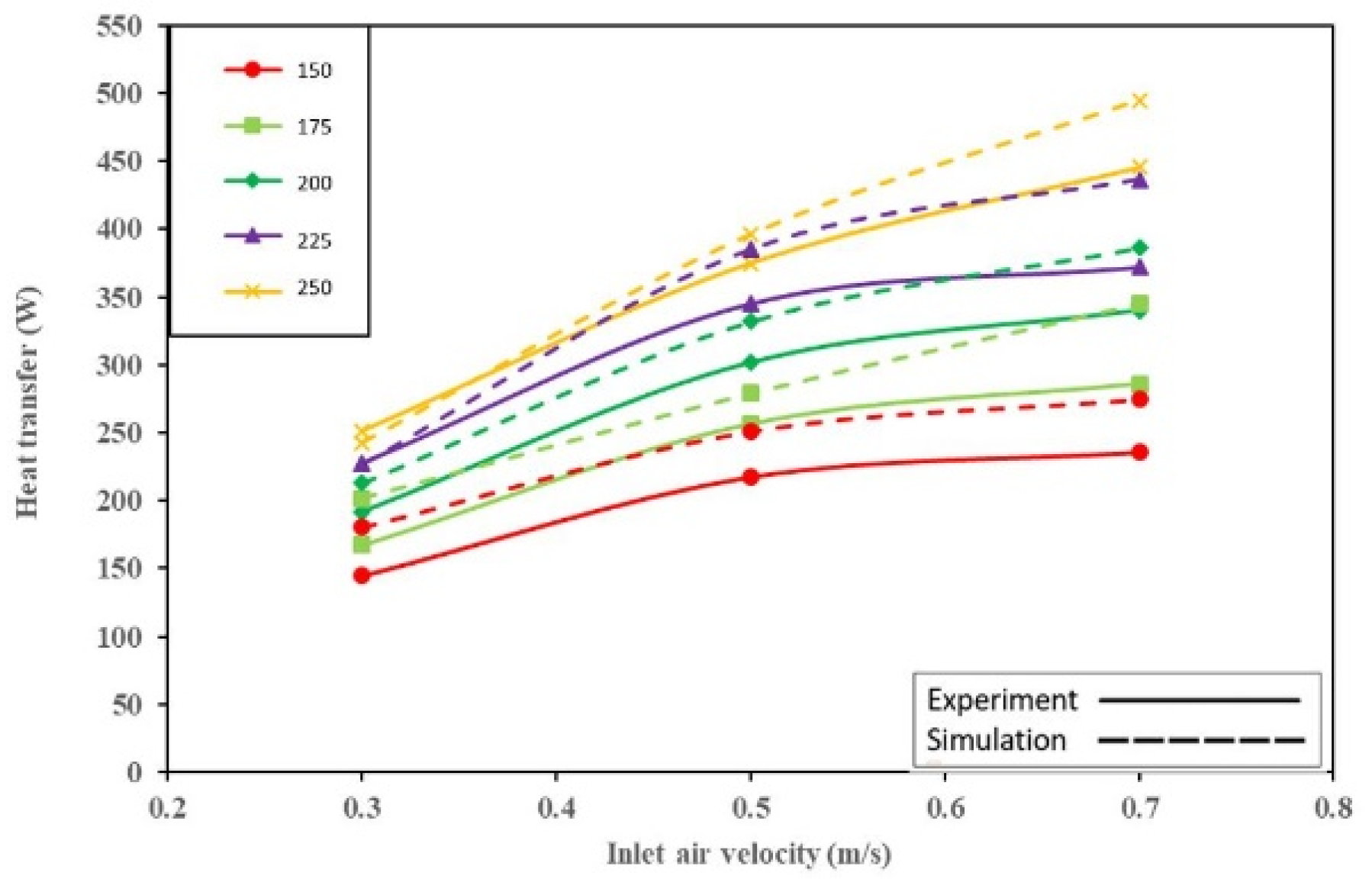
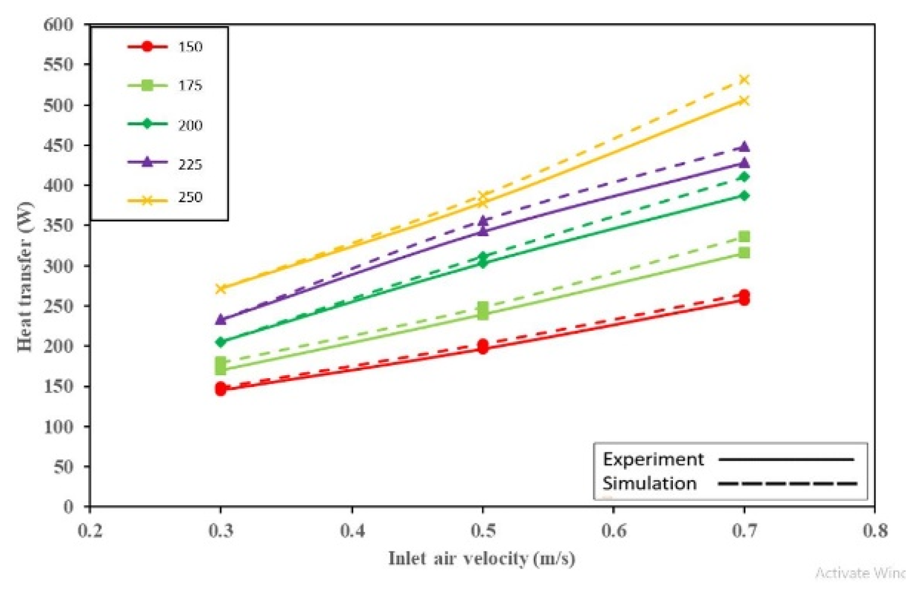
The inlet and outlet temperatures of the evaporator and condenser sections were used to calculate the heat transfer from the equations for the evaporator and condenser sections. The heat transfer from each side represents the heat taken from the hot air and transferred to cooling water simultaneously. The heat transfer also shows the energy balance of the device itself and during different loads. The heat transfer data for the hot side (q_h) and the heat transfer data for the cold section (q_c) are presented in Figure 11 and Figure 12, respectively. Figure 11 shows the q_h values for both the experimental and numerical sections, with comparisons to each other. The figure indicates that an increase in inlet air velocity and temperature also increased the heat transfer rate. For the maximum heat transfer, one should maintain a higher temperature of the inlet air. Meanwhile, if the temperature is lower, it is better to increase the inlet velocity of the air. The figure generally demonstrates that the maximum heat transfer from the experimental side was 503 W and from the numerical analysis side was 524 W. The difference between the systems was small and did not deviate more than ±21 W and the overall trend for the heat transfer remained constant with different input velocities of air. The hot-side heat transfer represents the thermal difference made by the cooler and does not represent the actual heat taken out. For the actual heat transfer of the device, we can use the cooler side of the heat transfer, which is lower and is calculated from the fluid with a higher heat capacity.

Figure 12 shows the heat transfer from the condenser side and the heat taken from the hot air. The figure shows both the numerical and experimental data q_c, with a comparison. The results on the condenser side show the same trend of the heat transfer increase with the increase in inlet air temperature and velocity. By studying the figure, we can see the trends of the experimental data, which are very consistent with respect to the input variables. The maximum heat transfer from the condenser side, according to the experimental analysis, was 445 W and the heat transfer increased in proportion to the inlet temperature and the inlet velocity of air. The data from the numerical analysis are within the range of the normal difference for the real-life heat transfer data obtained from experiments. The maximum heat transfer from the numerical analysis was 495 W and the maximum difference between the data obtained from the two approaches was not greater than ±50 K. The trend from the heat transfer data in the numerical analysis was not consistent, but it was always higher than that of the experimental analysis. This result indicates that even through the heat transfer was higher than the real-life results, the smaller deviation observed for the device can be interpreted to be similar to the experimental results. The results were inconsistent but can be studied further in order to improve them from the design perspective. The numerical analysis indicated that, overall, heat transfer values increased with the increase in the temperature and velocity of inlet air.

5. Conclusions

This study was performed on a heat pipe heat exchanger with the target of recovering energy from waste heat by supplying cooling water constantly. The experimental and numerical analyses were performed with waste heat of five different temperatures and three different inlet velocities. The overall change in temperature, the heat transfer of both the hot and cold sides, the outlet temperature and effectiveness were observed. The results of both the sections were compared and discussed. The following conclusions can be drawn from this study.

• In this study, we have presented the design of a heat exchanger for the recovery of waste heat by implementing a novel heat pipe made for a specific case. The novel heat pipe, with a stainless steel exterior and copper mesh, shows a great heat transfer ability with better future reliability than copper heat pipes.
• The study showed an increase in heat transfer with an increase in the inlet air temperature and velocity. One variable can be increased for a specific application in order to obtain the maximum heat transfer.
• The heat transfer capability of the device also increased with the increase in the inlet hot air temperature and velocity. For the experimental analysis, the maximum heat transfer was 445 W and lowest was 145 W, whereas for the numerical analysis, the maximum heat transfer was 495 W and the lowest heat transfer was 278 W.
• In the experiments, when the inlet velocity of hot air increased, the water temperature increased. The maximum effectiveness of the experimental results was 0.609, and the minimum was 0.410. The best input variable to adjust in response to a low heat transfer is to reduce the input air velocity in order to obtain greater effectiveness, whereas the velocity should be increased in order to achieve the maximum heat transfer.
• The comparison between the experimental and numerical results showed that the numerical results were on par with the experimental results, with the largest difference in heat transfer being 12%. The heat transfer obtained from the numerical analysis was higher because the losses in real-life situations were not compensated for in the analysis software.
• The numerical analysis was tested and was considered to accurately predict the behaviour of different parameters and the performance of the heat exchanger. By making various changes in input variables, one can develop a design which will suit the requirements according to the application needed. The method represents a cost- and time-effective solution for future development.