Flexible Design and Operation of Multi-Stage Flash (MSF) Desalination Process Subject to Variable Fouling and Variable Freshwater Demand

Said Alforjani Said; Mansour Emtir; Iqbal M. Mujtaba

doi:10.3390/pr1030279

,

and

¹

Maintenance and Projects Department, National Oil Corporation, P.O. Box 2655, Tripoli 00, Libya

²

Industrial Department, National Oil Corporation, P.O. Box 2655, Tripoli 00, Libya

³

School of Engineering Design & Technology, University of Bradford, Bradford, West Yorkshire BD7 1DP, UK

^*

Author to whom correspondence should be addressed.

Processes2013, 1(3), 279-295;https://doi.org/10.3390/pr1030279

This article belongs to the Special Issue Feature Papers

Version Notes

Order Reprints

Abstract

This work describes how the design and operation parameters of the Multi-Stage Flash (MSF) desalination process are optimised when the process is subject to variation in seawater temperature, fouling and freshwater demand throughout the day. A simple polynomial based dynamic seawater temperature and variable freshwater demand correlations are developed based on actual data which are incorporated in the MSF mathematical model using gPROMS models builder 3.0.3. In addition, a fouling model based on stage temperature is considered. The fouling and the effect of noncondensable gases are incorporated into the calculation of overall heat transfer co-efficient for condensers. Finally, an optimisation problem is developed where the total daily operating cost of the MSF process is minimised by optimising the design (no of stages) and the operating (seawater rejected flowrate and brine recycle flowrate) parameters.

Keywords:

freshwater demand; storage tank; dynamic optimisation; total operating cost

1. Introduction

At present, there is a shortage in the freshwater resources all over the world. About 40% of the world’s populations are suffering from the water crisis. This is due to the continuous growth of the world population and economic activities. Moreover, 96% of the water on the earth is located in oceans and seas and out of 1.7% groundwater only 0.8% is considered to be the freshwater [1]. Desalination is a technique of producing freshwater from saline water. Industrial desalination of sea water is becoming an essential part in providing sustainable source of freshwater for a large number of countries around the world [2]. Among different desalination processes, thermal process is the oldest and most dominating for large scale production of freshwater in today’s world. Amongst various thermal processes, the Multi-Stage Flash (MSF) distillation process has been used for many years and now is one of the largest sectors in the desalination industry.

During the last decades, modelling played a very important role in the simulation, optimisation and control of multistage flash (MSF) desalination process. Many models have been developed to find a functional relationship between the design and operating variables [3]. For a given design, optimisation of operating variables led to an increase in distillate production rates and lower operating costs. The top brine temperature, brine recirculation rate, intake flow rate, and steam condition and flow rate can be manipulated to enhance plant performance and achieve an incremental increase in plant capacity. In addition, the selection of optimum design and operation of MSF desalination is aimed at reducing energy and operation costs such as steam, electric power, anti-scale, etc.

A recent study [4] shows that for a fixed design and operating conditions the production of fresh water from MSF process can significantly vary with seasonal variation of seawater temperature producing more water in winter than in summer. However, the freshwater demand is continuously increasing and of course there is more demand in summer than in winter. Furthermore, to supply freshwater meeting a fixed demand, the operation of MSF process has to be adjusted with the variation of seawater temperature to reduce the energy and operation cost such as steam and antiscale [5,6]. Also, apart from seasonal variation, the seawater temperature varies during the day [7]. More importantly, there is variation in water demand during 24 h of a day (peak and off-peak hours) [8]. These variations in the seawater temperature will affect the rate of production of freshwater using MSF process during a day and throughout the year. Therefore, an optimal design and operation of MSF processes should be performed to cope with these variations so that the freshwater demand during a day and throughout the year is maintained.

Most recently, [9] provided a study on the design and operation of the MSF process with constant fouling resistance in the brine heater only and variable seawater temperature and freshwater demand during a day and throughout the year. However, the dynamic variation in freshwater demand during the week days is not the same as weekends [10]. Also, the changing seawater temperature during the day will affect the stage temperature which will affect the fouling profile of the stages. Unlike Hawaidi and Mujtaba [9], we have proposed a fouling model [11,12] as a function of stage temperature which is incorporated into the MSF process model. In addition to fouling, the effect of non-condensable gases [13] on the condenser overall heat transfer co-efficient is built up in the process model. Like Hawaidi and Mujtaba [9], an intermediate storage tank between the plant and the client is considered to provide additional flexibility in operation and maintenance of the MSF process throughout the day. However, instead of a neural network based freshwater demand model, simple polynomial based dynamic freshwater demand correlation is developed using actual data from literature. These correlations with a dynamic model for the storage tank and the CaCO₃ fouling resistance model developed earlier [11,12] are incorporated in the full steady state MSF mathematical model by using gPROMS model builder 3.0.3 [14]. For a different number of flash stages, operating parameters such as seawater rejected flow rate and brine recycle flow rate are optimised, while the total daily operating cost of the MSF process is selected to minimise.

2. Dynamic Freshwater Demand

Figure 1 shows the average freshwater consumption for the 24 h of a weekend (Saturday) [10]. The average consumption slopes down from 0.00 to 6.00 and grows up from 6:00 am till 12:00 am. From 14:00 the curve goes down till 24:00. In addition and by using linear regression analysis, the following polynomial relationship (Equation (1)) is obtained with a correlation coefficient greater than 90%.

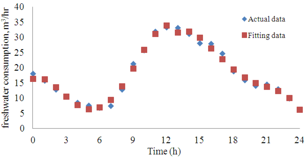
Figure 1. Fresh water consumption profile on holiday (Saturday).

(1)

3. Seawater Temperature Dynamic Profiles

The variation in seawater temperature throughout the day is shown in Figure 2 [7]. By using regression analysis, the relationship between the seawater temperature and time (h) can be represents by Equation (13). The temperature at t = 0 represents the seawater temperature at night-time.

(2)

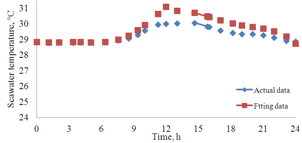
Figure 2. Seawater temperature profile during the day and night.

Note, between 0 and 10 h, 5th order polynomial shows a very good mapping with the actual data. Beyond 10 h, although the polynomials do not show a close map, the trend of temperature change is retained.

4. MSF Process Model

4.1. MSF Process Description

The MSF process mainly consists of three sections: brine heater section, recovery section with NR stage and rejection sections with NJ stage (Figure 3). Seawater enters into the last stage of the rejection stages (W_S) and passes through series of tubes to remove heat from the stages. Before the recovery section seawater is partly discharged to the sea (C_W) to balance the heat. The other part (F) is mixed with recycled brine (R) from the last stage of the rejection section and fed (W_R) before the last stage of the recovery section. Seawater is flowing through the tubes in difference stages to recover heat from the stages and the brine heater raises the seawater temperature to the maximum attainable temperature (Top brine temperature TBT). After that it (B₀) enters into the first flashing stage and produce flashing vapour. This process continues until the last stage of the rejection section. The concentrated brine (B_N) from the last stage is partly discharged to the sea (B_D) and the remaining (R) is recycled as mentioned before. The vapour from each stage is collected in a distillate tray to finally produce the fresh water (D_N). Vapour from each stage is collected in a distillate tray to finally produce the fresh water (D_N).

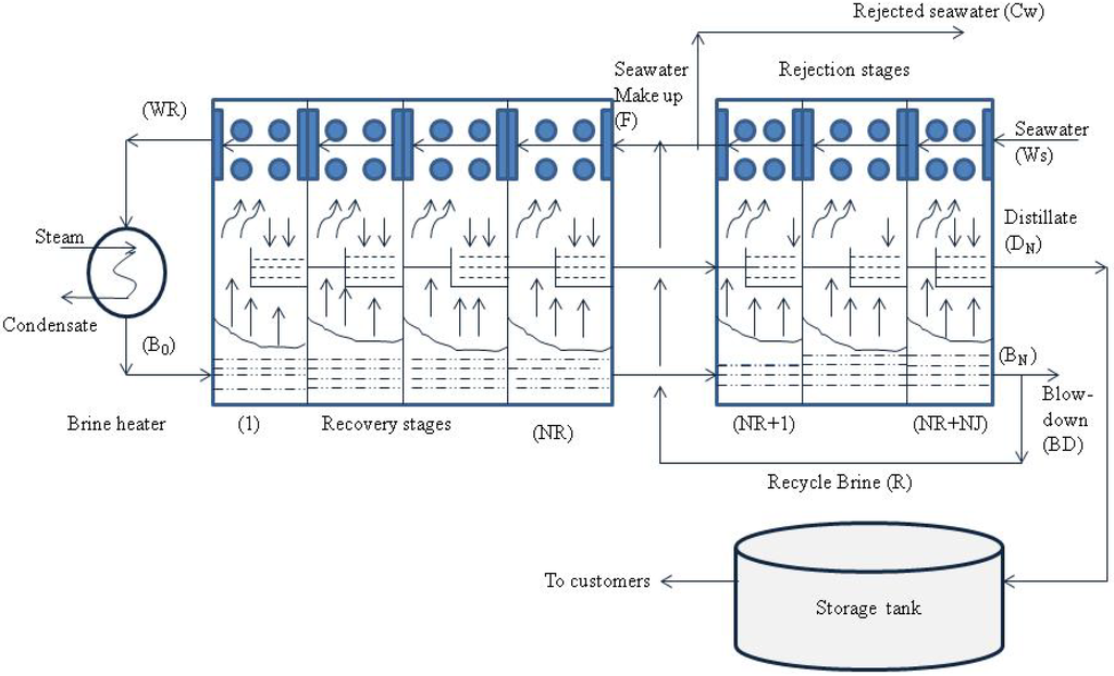
Figure 3. Typical Multi-Stage Flash (MSF) Process.

4.2. Steady State MSF Process Model

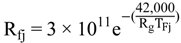
With reference to Figure 3, models for flash stages; brine heater, mixers, splitter, etc., are developed using gPROMS software. The steady state model is based on the total and component mass balances and enthalpy balances coupled with heat and mass flowrate coefficients. The model also includes the thermodynamic losses from stage to stage, tube velocity, tube materials, and chamber geometry. The model equations presented here are reported by [13,15]. The physical properties correlations are defined in the original references [15,16,17]. Note, a calcium carbonate fouling resistance model (Equation (11)) has been implemented in the MSF steady state model in this work. This model takes into consideration the effect of stage temperature on the calcium carbonate fouling resistance and consequently on the overall heat transfer coefficient in the flashing champers in the heat recovery section, heat rejection section, and brine heaters of MSF process at fluid velocity 1 m/s.

The following assumptions are made in the model:

The distillated from any stage is salt free
Heat of mixing are negligible
No sub cooling of condensate leaving the brine heater
There are no heat losses and
There is no entrainment of mist by the flashed vapour.

The model equations are presented below for the sake of completeness.

4.2.1. Stage Model

Mass Balance in the flash chamber:

(3)

Mass Balance for the distillate tray:

(4)

Enthalpy balance on flash brine:

(5)

(6)

(7)

Overall Energy Balance:

(8)

Heat transfer equation:

(9)

(replace W_R for W_S rejection stage)

(10)

Where,

(11)

(12)

(13)

The logarithmic mean temperature difference in the recovery and rejection stages:

(14)

(replace W_R for Ws rejection stage)

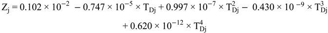
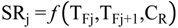
Heat capacity of cooling brine leaving stage j:

(15)

Heat capacity of distillate leaving stage j

(16)

Heat capacity of flashing brine leaving stage j

(17)

Distillate and flashing brine temperature correlation:

(18)

Distillate and flashing steam correlation:

(19)

Temperature loss due to demister

(20)

Boiling point elevation at stage j

(21)

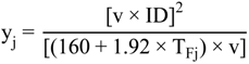
Non-equilibrium allowance at stage j

(22)

4.2.2. Brine Heater Model

Mass and salt balance for the brine heater

(23)

(24)

Overall enthalpy balance

(25)

(26)

Heat transfer equation

(27)

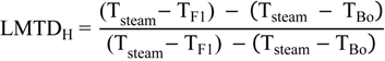
The logarithmic mean temperature difference in brine heater (LMTD_H)

(28)

Overall heat transfer coefficient in brine heater

(29)

Heat capacity of brine in brine heater

(30)

4.2.3. Splitter Model

Mass balance on seawater splitter

(31)

(32)

4.2.4. Mixers Model

Mass balance on mixer

(33)

(34)

Enthalpy balance on mixer:

(35)

(36)

(37)

5. Storage Tank and Level Control Models

These models are taken from Hawaidi and Mujtaba [9] and are presented here for the sake of completeness of the process model.

5.1. Storage Tank Model

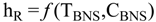
The dynamic mathematical model of the tank process shown in Figure 4 is as the follows: Mass balance

(38)

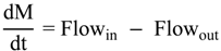Relation between liquid level and holdup:

(39)

Note, Flow_out represents the freshwater demand described by Equation (1).

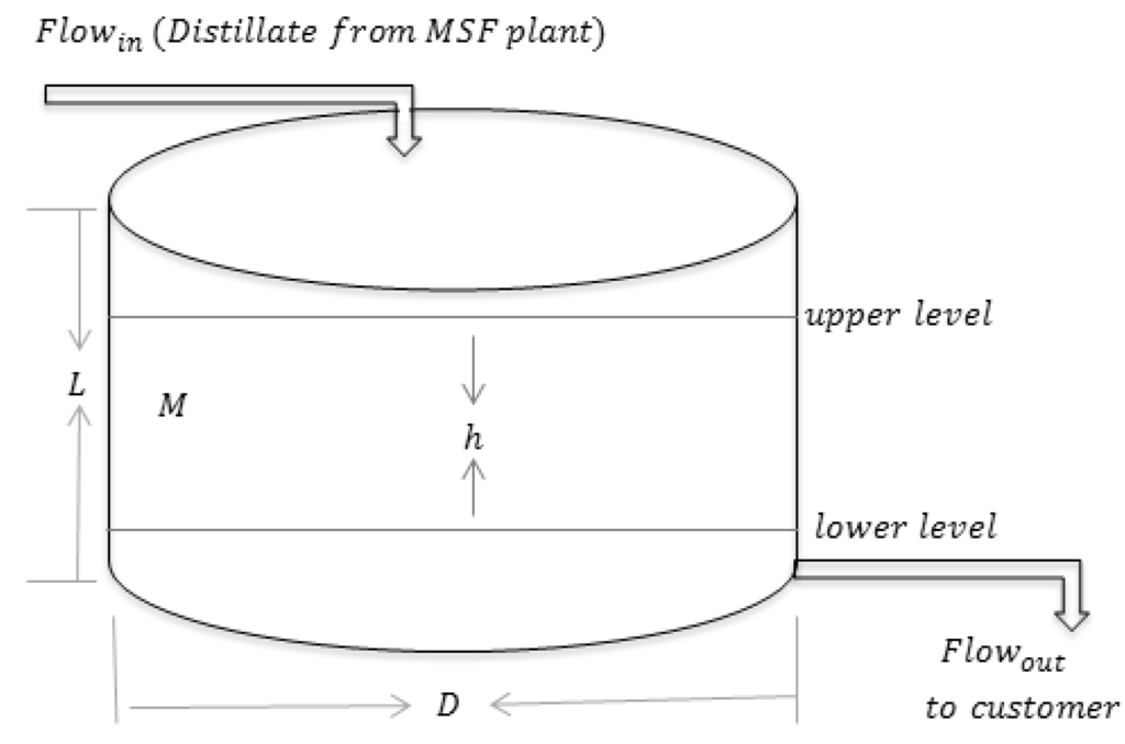
Figure 4. Storage tank.

5.2. Storage Tank Level Control Model

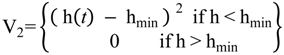
The storage tank described above is assumed to operate without any control on the level(h), therefore and during the MSF operation process, the tank level goes above the maximum level (h_max) or below the minimum level (h_min) as shown in Figure 5(a). At any time, this violation (V₁, V₂) of safe operation can be defined as [9]:

(40)

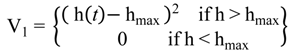and

(41)

A typical plot of V₁ and V₂ versus time t is shown in Figure 5(b). The total accumulated violation for the entire period can be written using

(42)

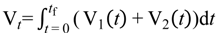Therefore,

(43)

Equation (43) is added to the overall process model equations. Also the following addition terminal constraint is added in the optimisation problem formulations.

(44)

where ε is a very small finite positive number. The above constraint will ensure h(t) that will always be ≤h_max and ≥h_min throughout the 24 h operation.

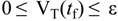
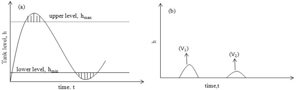
Figure 5. (a) Tank level profile and (b) tank level violations during the MSF operation.

6. Optimisation of MSF Parameters

The seawater temperature and the freshwater demand are subject to vary during a day. Therefore, to supply freshwater meeting a variation in the seawater temperature and variable freshwater demand throughout the day, the operation parameters of the MSF process has to be adjusted. In this section, the MSF process model and the CaCO₃ fouling resistance model coupled with the storage tank model developed has been used to adequate the variations in the seawater temperature and freshwater demand during a day. For different number of flash stages, operating parameters such as seawater rejected flow rate and brine recycle flow rate are optimised, while the total annual operating cost of the MSF process is selected to minimise using gPROMS models builder 3.0.3 (version 3.0.3.; PSE: London, UK).

Optimisation Problem Formulation

The optimisation problem is described as:

Given: Design specifications of each stage, fixed amount of seawater flow, heat exchanger areas in stages, variable seawater temperature, steam temperature, freshwater demand profile, and volume of the storage tank.

Optimise: Recycle brine flow rate, rejected seawater flow rate, at different time intervals within 24 h.

To minimise: The total operation cost (TOC, $/day).

The optimisation problem (OP) can be described mathematically by:

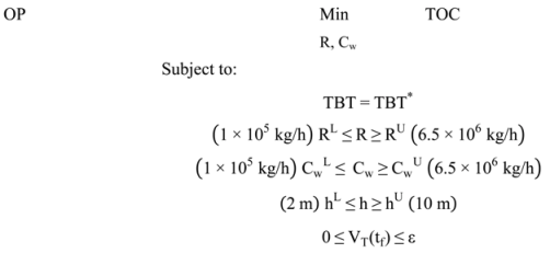Where, is the top brine temperature and TBT^* is the fixed top brine temperature. R is the recycle flowrate and C_w is the rejected seawater flowrate. Subscripts L and U refer to lower and upper bounds of the parameters.

The objective function, TOC (total operating cost) is defined as [18]:

(45)

Where,

(46)

Where, W_S is steam consumption in kg/hr, T_s is steam temperature in °C

(47)

Where, W_M is make-up flow rate in kg/hr, ρ_B is brine density in kg/m³

(48)

Where, W_d is distillate product in kg/hr, ρ_w is water density in kg/m³

(49)

(50)

This optimisation problem minimises the total operating cost while optimises R and C_w for variable seawater temperature and freshwater demand throughout 24 h. Note, the actual freshwater consumption at any time is assumed to be 40,000 times more than that shown in Figure 1.

7. Case Study

A steady state process model for the MSF process coupled with a dynamic model for the storage tank (as described earlier) has been used in the case study. The constant parameters of the MSF process model equations including various dimensions of the brine heater and flash stages are listed in Table 1. The rejection section consists of three stages but the number of stages in the recovery section varies in each case (see Table 2) considered here. The feed seawater flow rate is 1.13 × 10⁷ kg/h with salinity 5.7 wt. %. The intermediate storage tank has diameter D = 18 m, and aspect ratio = L/D = 0.5.

Table 1. Constant parameters.

**Table 1.** Constant parameters.
Unit	A_j/A_H	D_jⁱ/D_Hⁱ	D_j⁰/D_H⁰	w_j/L_j/L_H	H_j
Brine heater	3530	0.022	0.0244	12.2
Recovery stage	3995	0.022	0.0244	12.2	0.457
Rejection stage	3530	0.024	0.0254	10.7	0.457

Table 2. Summary of optimisation results.

**Table 2.** Summary of optimisation results.
Case	N	C1, $/d	C2, $/d	C3, $/d	C4, $/d	C5, $/d	TOC, $/d
1	16	46,184,583	37,498,047	17,220,256	12,954,688	15,798,400	129,655,973
2	17	44,026,301	37,597,628	17,358,817	13,058,927	15,925,521	127,967,194
3	18	41,403,746	37,222,956	17,250,642	12,977,547	15,826,277	124,681,167

Six time intervals within 24 h are considered within which both R and C_W are optimised with the interval lengths. The total operating cost on daily basis and the other plant cost (steam cost (C1), chemical cost (C₂), power cost (C₃), spare cost (C₄) and labour cost (C₅)) for three different number of stages (16, 17 and 18) are listed in Table 2. The total daily operating cost (TOC represented as $/day) is found to decrease as the number of stage increases. This is due to lower steam consumption rate with increasing number of stages contributing significantly to the TOC compared to any other cost components (chemical, power, etc.). Note, there is a small change in the C₂, C₃, C₄ and C₅ while a change in the C1 is relatively high (Table 2).

Figure 6 shows the stage temperature (calculated using the process model) and fouling resistance (calculated using Equation (11)) at different stages for N = 18 and seawater temperature at time t = 00:00. The fouling resistance in stage 1 is about 300 times more than that in stage 1 and certainly it will affect the overall heat transfer co-efficient profile (calculated using Equation (10)) significantly. Figure 6 clearly shows that the fouling resistance is not constant throughout the stages as considered earlier by Hawaidi and Mujtaba [9] and Rosso et al. [15].

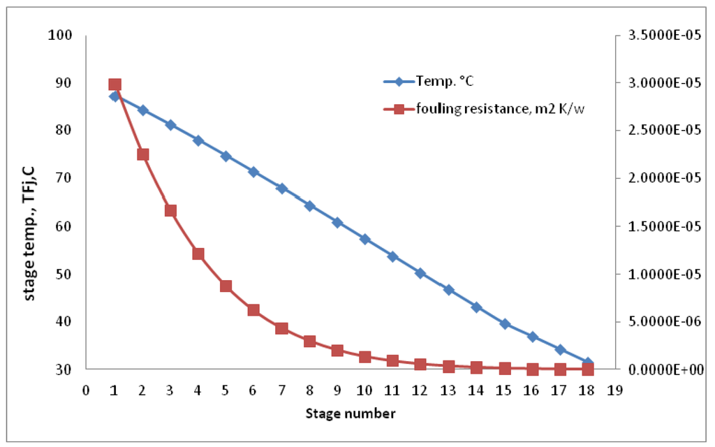
Figure 6. Stage temperature and fouling profile (N = 18). Note: In y axis, E+00 = 10⁰; E−06 = 10⁻⁶ and likewise.

Figure 7 and Figure 8 show the optimum results of seawater rejected flow rate (C_w) and recycle flow rate (R) throughout 24 h at different number of stages. The plant operates at the high flow rate of C_w (Figure 7) and low R (Figure 8) from 00:00 to 08:00 when the water production rate is low due to low water demand (Figure 9 and Figure 10). However, the water production rate is sufficient to cover the demand (decreasing between 00:00 and 05:00) as well as to store meeting the increasing demand (beyond 06:00) (Figure 10 and Figure 11).

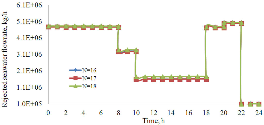
Figure 7. Optimum rejected seawater flow rate throughout profile. Note: In y axis, E+05 = 10⁵ and likewise.

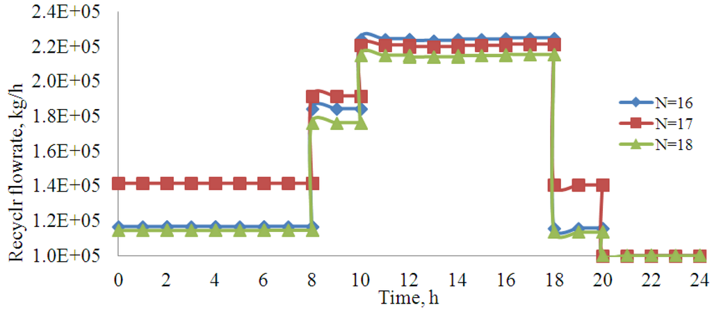
Figure 8. Optimum brine recycle flow rate throughout profile. Note: In y axis, E+05 = 10⁵ and likewise.

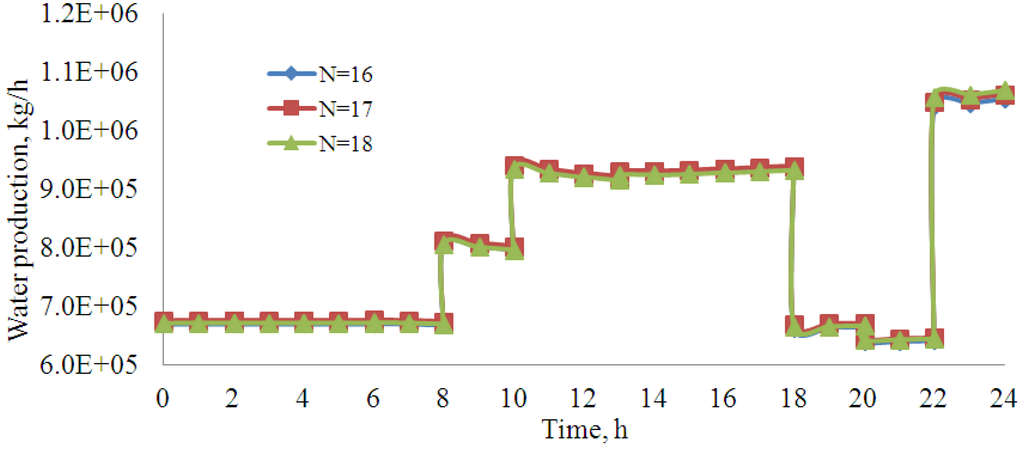
Figure 9. Fresh water plant production profile. Note: In y axis, E+05 = 10⁵ and likewise.

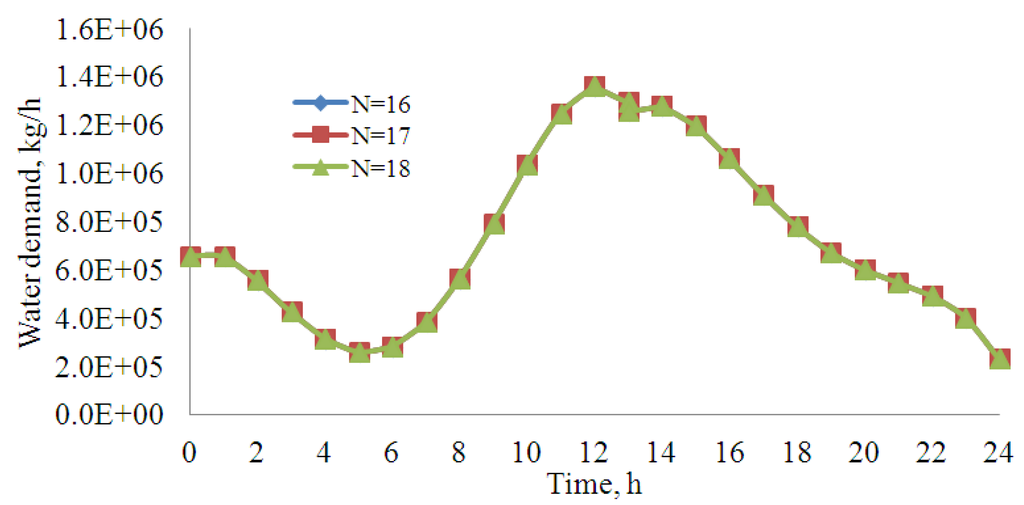
Figure 10. Fresh water demand profile. Note: In y axis, E+05 = 10⁵ and likewise.

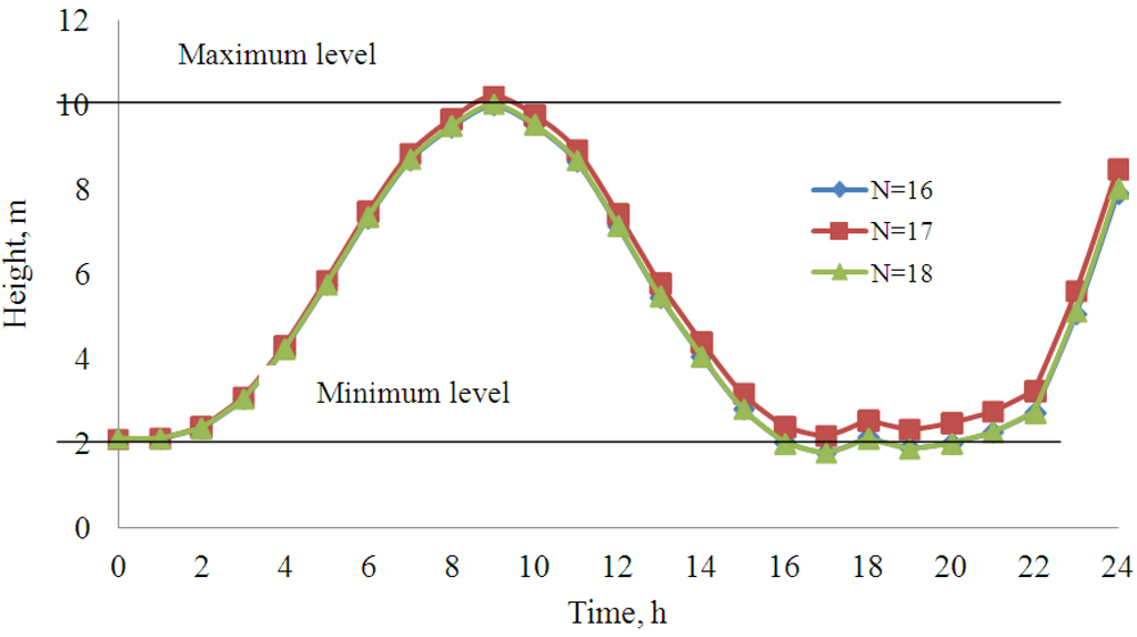
Figure 11. Storage tank level profiles (case 1).

As the water demand increases between 05:00 and 12:00 (Figure 10), C_w and R reverse their profiles (Figure 7 and Figure 8) to increase the water production rate (Figure 9). Interestingly, up to 09.00, the water production rate is still more than the demand (thus increasing the storage tank level). Beyond 09:00, the water production rate is not sufficient to meet the demand and therefore it is being subsidized from the stored water (thus decreasing the tank level) (Figure 11). Although, the water demand drops down beyond 12:00, the trend of C_w, R and water production rate continues at the same level right up to 18:00. During this period, storage tank level continues to drop down to the minimum. Beyond 18:00 C_w are R are adjusted to have sufficient water production to meet the demand until 24:00 and to store at the same time.

However, the intermediate storage tank adds the operational flexibility, and maintenance could be carried out without interrupting the production of water or full plant shut-downs at any time throughout the day by adjusting the number of stage. Note, the optimal results in this case are almost the same for the all the number of stages considered.

8. Conclusions

In this work, for a given design, an optimal operation scheme for an MSF desalination process subject to variable seawater temperature and variable freshwater demand is considered. An intermediate storage tank is considered between the MSF process and the customer to add flexibility in meeting the customer demand. A dynamic model for the storage tank level has been implemented with steady state MSF process model using gPROMS 3.0.3 model builder. Unlike previous work, a stage temperature based fouling correlation is added and the effect of non-condensable gases on the condenser heat transfer co-efficient is reflected into the process model.

For several process configurations (the design), some of the operation parameters of the MSF process such as seawater recycle flow rate and brine recycle flow rate at discrete time interval are optimised, while minimising the total daily operating costs. The optimisation results show increase in the total operating cost with decreasing number of stages. During the low consumption of freshwater, there is an increase in the tank level and plant production. Consequently, the plant operates at maximum value of rejected seawater flowrate and at minimum value of recycled brine flowrate. On the other hand, optimum results show decrease in the plant production and tank level when there is an increase in the freshwater consumption and consequently the plant operate at minimum value of rejected seawater flowrate and slightly increase in recycled brine flowrate. The results also clearly show that the use of the intermediate storage tank adds flexible scheduling in the MSF plant to meet the variation in freshwater demand with varying seawater temperatures without interrupting or fully shutting down the plant at any time during the day by connecting the desired number of stages (see [19] for the concept).

Nomenclature

A_H	Heat transfer area of brine heater (m²)
A_j	Heat transfer area of stage j (m²)
A_S	cross sectional area of storage tank (m²)
B₀	Flashing brine mass flow rate leaving brine heater (kg/h)
BBT	Bottom brine temperature (°C)
B_D	Blow-down mass flow rate (kg/h)
B_j	Flashing brine mass flow rate leaving stage j (kg/h)
C_B0	Salt concentration in flashing brine leaving brine heater (wt. %)
C_Bj	Salt concentration in flashing brine leaving stage j (wt. %)
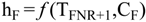
C_BNS	Salt concentration in brine recycle (R) (wt. %)
C_R	Salt concentration in feed seawater (WR) (wt. %)
C_S	Salt concentration in makeup seawater (F) (wt. %)
C_W	Rejected seawater mass flow rate (kg/h)
D_j	Distillate flow rate leaving stage j (kg/h)
D	Diameter of storage tank (m)
EX_j	Non-equilibrium allowance at stage j
F	Make-up seawater mass flow rate (kg/h)
f_j^H	Brine heater fouling factor ( h m² °C/kcal)
f_jⁱ	Fouling factor at stage j ( h m² °C/kcal)
h	freshwater level in the storage tank (m)
h_Bj	Specific enthalpy of flashing brine at stage j (kcal/kg)
h_R	Specific enthalpy of flashing brine at T_F (kcal/kg)
h_vj	Specific enthalpy of flashing vapor at stage j (kcal/kg)
h_W	Specific enthalpy of brine at T_F (kcal/kg)
H_j	Height of brine pool at stage j (m)
L_H	Length of brine heater tubes (m)
L	Length of storage tank (m)
L_j	length of tubes at stage j (m)
M	storage tank holdup
ID	Internal diameter of tubes (m)
OD	External diameter of tubes (m)
W_steam	Steam mass flow rate (kg/h)
R	Recycle stream mass flow rate (kg/h)
SB_j	Heat capacity of flashing brine leaving stage j (kcal/kg/°C)
SD_j	Heat capacity of distillate leaving stage j (kcal/kg/°C)
SR_j	Heat capacity of cooling brine leaving stage j (kcal/kg/°C)
TBT	Top brine temperature (°C)
T_Bj	Temperature of flashing brine leaving stage j (°C)
T_BNS	Temperature of the brine in the recycle flowrate (°C)
T_BO	Temperature of flashing brine leaving brine heater (°C)
T_Dj	Temperature of distillate leaving stage j (°C)
TE_j	Boiling point elevation at stage j (°C)
T_Fj+1	Temperature of cooling brine leaving stage j (°C)
T_FNR+1	Temperature of makeup flowrate (F) (°C)
T_Fm	Temperature of the brine in feed entering recovery stage (°C)
T_Vj	Temperature of flashed vapour at stage j (°C)
T_steam	Steam temperature (°C)
T_seawater	Seawater temperature (°C)
U_H	Overall heat transfer coefficient at brine heater (Kcal/m² h K)
U_j	Overall heat transfer coefficient at stage j (Kcal/m² h K)
ww_j	Width of stage j (m)
W_S	Seawater mass flow rate (kg/h)
X	LMTD, logarithmic mean temperature difference at stages
Y	LMTD, logarithmic mean temperature difference at brine heater
Δ_j	Temperature loss due to demister (°C)
ρ_j	Brine density (kg/h)
λ_s	Latent heat of steam to the brine heater (kcal/kg)

IDEX

H	Brine heater
j	Stage index
*	Reference value

Conflicts of Interest

The authors declare no conflict of interest.

References

Assiry, A.M.; Gaily, M.H.; Alsamee, M.; Sarifudin, A. Electrical conductivity of seawater during ohmic heating. Desalination 2010, 260, 7–19. [Google Scholar]
El-Dessouky, H.T.; Eltouney, H.M. Fundamentals of Salt Water Desalination; Elsevier Science, Ltd.: Amsterdam, The Netherlands, 2002. [Google Scholar]
Alasfour, F.N.; Abdulrahim, H.K. Rigorous steady state modeling of MSF-BR desalination system. Desalin. Water Treat. 2009, 1, 259–276. [Google Scholar] [CrossRef]
Tanvir, M.S.; Mujtaba, I.M. Optimisation of MSF desalination process for fixed water demand using gPROMS. Comput. Aided Chem. Eng. 2007, 24, 763. [Google Scholar] [CrossRef]
Tanvir, M.S.; Mujtaba, I.M. Optimisation of design and operation of MSF desalination process using MINLP technique in gPROMS. Desalination 2008, 222, 419–430. [Google Scholar] [CrossRef]
Hawaidi, E.A.; Mujtaba, I.M. Freshwater production by MSF desalination process: Coping with variable demand by flexible design and operation. Comput. Aided Chem. Eng. 2011, 29, 1180–1184. [Google Scholar] [CrossRef]
Yasunaga, K.; Fujita, M.; Ushiyama, T.; Yoneyama, K.; Takayabu, Y.N.; Yoshizaki, M. Diurnal variations in precipitable water observed by shipborne GPS over the tropical indian ocean. SOLA 2008, 4, 97–100. [Google Scholar] [CrossRef]
Alvisi, M.A.; Franchini, M.; Marinelli, A. A short-term pattern-based model for water-demand forecasting. J. Hydroinform. 2007, 91, 39–50. [Google Scholar]
Hawaidi, E.A.; Mujtaba, I.M. Meeting variable freshwater demand by flexible design and operation of the Multistage Flash Desalination process. Ind. Eng. Chem. Res. 2011, 50, 10604–10614. [Google Scholar] [CrossRef]
Herrera, M.; Torgo, L.; Izquierdo, J.; Perez-Garcıa, R. Predictive models for forecasting hourly urban water demand. J. Hydrol. 2010, 387, 141–150. [Google Scholar] [CrossRef]
Said, S.; Mujtaba, I.M.; Emtir, M. Effect of Fouling Factors on the Optimisation of MSF Desalination Process for Fixed Water Demand Using gPROMS. In Proceeding of the 9th International Conference on Computational Management, London, UK, 18–20 April 2012.
Said, S.A. MSF Process Modelling, Simulation and Optimisation: Impact of Noncondensable Gases and Fouling Factor on Design and Operation. Ph.D. Thesis, University of Bradford, Yorkshire, UK, 2012. [Google Scholar]
Said, S.; Mujtaba, I.M.; Emtir, M. Modelling and simulation of the effect of non-condensable gases on heat transfer in the MSF desalination plants using gPROMS software. Comput. Aided Process Eng. 2010, 28, 25–30. [Google Scholar] [CrossRef]
gPROMS. In gPROMS User Guide 2005; Process System Enterprise, Ltd. (PSE): London, UK, 2005.
Rosso, M.; Beltramini, A.; Mazzotti, M.; Morbidelli, M. Modelling of multistage flash desalination plants. Desalination 1996, 108, 365–374. [Google Scholar]
Helal, A.; Medani, M.; Soliman, M.; Flower, J. Tridiagonal matrix model for multistage flash desalination plants. Comput. Chem. Eng. 1986, 10, 327–342. [Google Scholar] [CrossRef]
Hussain, A.; Hassan, A.; Al-Gobaisi, D.; Al-Radif, A.; Woldai, A.; Sommariva, C. Modeling, simulation, optimization and control of multistage flash (MSF) desalination plants Part2: Modeling and simulation. Desalination 1993, 92, 21–41. [Google Scholar] [CrossRef]
Helal, A.M.; El-Nashar, A.M.; Al-Kahtheeri, E.; Al-Malek, S. Optimal design of hybrid RO/MSF desalination plants Part I: Modeling and algorithms. Desalination 2003, 154, 43–66. [Google Scholar] [CrossRef]
Sowgath, T.; Mujtaba, I.M. Less of the foul play: Flexible design and operation can cut fouling and shutdown of desalination plants. tce 2008, June, 28–29. [Google Scholar]

© 2013 by the authors; licensee MDPI, Basel, Switzerland. This article is an open access article distributed under the terms and conditions of the Creative Commons Attribution license (http://creativecommons.org/licenses/by/3.0/).