Abstract
Environmental changes and sensor aging can cause sensor drift in sensor array responses (i.e., a shift in the measured signal/feature distribution over time), which in turn degrades gas classification performance in real-world deployments of electronic-nose systems. Previous studies using the UCI Gas Sensor Array Drift Dataset as a benchmark reported promising drift compensation results but often lacked robust statistical validation and may overcompensate for drift by suppressing class-discriminative variance. To address these limitations and rigorously evaluate improvements in sensor-drift compensation, we designed two domain adaptation tasks based on the UCI electronic-nose dataset: (1) using the first batch to predict remaining batches, simulating a controlled laboratory setting, and (2) using Batches 1 through to predict Batch n, simulating continuous training data updates for online training. Then, we systematically tested three methods—our semi-supervised knowledge distillation method (KD) for sensor-drift compensation; a previously benchmarked method, Domain-Regularized Component Analysis (DRCA); and a hybrid method, KD–DRCA—across 30 random test-set partitions on the UCI dataset. We showed that semi-supervised KD consistently outperformed both DRCA and KD–DRCA, achieving up to 18% and 15% relative improvements in accuracy and F1-score, respectively, over the baseline, proving KD’s superior effectiveness in electronic-nose drift compensation. This work provides a rigorous statistical validation of KD for electronic-nose drift compensation under long-term temporal drift, with repeated randomized evaluation and significance testing, and demonstrates consistent improvements over DRCA on the UCI drift benchmark.
1. Introduction
Non-intrusive gas recognition is significant in research and industrial applications [1,2]. The electronic nose, an artificial olfactory system that mimics the mammalian olfactory system, offers a rapid and cost-effective approach for pattern recognition-based analysis of volatile organic compounds (VOCs) and gases [3,4]. It has been widely adopted for gas/VOC classification across a variety of application scenarios [4]. Its easy operation and low cost enhance its versatility and application fields [5]. Accurate identification and classification of gases using an electronic nose have numerous applications across various fields [6]: in environmental monitoring, electronic noses are used to assess air quality [7], and in food quality assessment, electronic noses are used to detect the gas composition of food to determine food quality [8]. For example, Wojnowski’s team used electronic noses to successfully classify poultry and canola oil samples and detect olive oil adulteration, achieving an overall accuracy of 82% [9]. In addition, electronic noses are used to detect the quality of beverages and medicinal herbs such as wine, coffee, ginseng, and Chinese medicine [10,11,12,13]. Furthermore, they are used to aid in disease diagnosis by analyzing volatile organic compounds in breath air [14,15]. Regarding pattern recognition software and algorithms, over the past two decades, with the development of machine learning, integrating pattern recognition algorithms, such as support vector machines, neural networks, and conformal prediction, has enabled electronic noses to perform accurate classification and regression analysis of various analytes [16,17,18]. For example, electronic-nose systems have been used to recognize explicitly defined gas-phase analytes and mixtures (e.g., components in industrial exhaust) using machine learning-based pattern recognition [19].
Although the electronic nose is a powerful tool for gas classification, it faces the critical challenge of sensor drift during deployment. Sensor drift can result from factors such as the aging of sensor materials, poisoning, and the accumulation of contaminants. Furthermore, environmental changes, including variations in humidity and temperature, can contribute to sensor drift [20]. These changes lead to variations in sensor response characteristics, which affect the robustness and accuracy of electronic-nose-based pattern recognition models over time or across environments [3,18]. Furthermore, sensor drift shows non-linear dynamic behavior in multi-dimensional sensor arrays, making it a challenging issue to address experimentally and computationally [21].
Sensor drift can be viewed as a domain adaptation problem in machine learning because it induces a distribution shift from a source domain (earlier batches collected by a sensor system) to a target domain (later batches collected by a sensor system). Although transfer learning and model fine-tuning can be used to adapt the model to new data distributions [22], they require supervised fine-tuning and labels in the new domains, which are hard to obtain in electronic-nose applications. This calls for unsupervised methods for drift compensation. Existing methods to address sensor drift can be categorized from a data perspective or from a model perspective. From a data perspective, domain adaptation methods are employed to align the data distributions between the target and source domains. As an example, Domain-Regularized Component Analysis (DRCA) seeks to mitigate the differences between the target and source domains by finding a domain-invariant feature subspace. By reducing these differences, DRCA can improve the generalizability of the model in the target domain. Previous studies have applied DRCA for sensor-drift compensation in electronic-nose systems, as well as other sensing modalities (e.g., IMUs and surface electromyography), and have reported improved cross-domain performance on target domain data [23,24,25]. Another data-perspective domain adaptation method, CycleGAN, transforms target domain samples to resemble the source domain, enabling source-trained models to be applied to target domain classification. In our previous work [25], we directly compared CycleGAN with DRCA under a domain adaptation setting and found that DRCA outperformed CycleGAN, likely due to overfitting in this low-sample, drift-prone scenario.
From a model perspective, domain adaptation methods adapt the source domain model to the target domain data distribution. As an example, knowledge distillation (KD) is a recently developed semi-supervised domain adaptation approach that improves model generalizability by transferring knowledge from a complex model (teacher model) to a simpler model (student model), preventing overreliance on the source domain and enabling better performance in the target domain [26]. Additionally, other semi-supervised learning approaches, such as reliability-based unlabeled data augmentation and training data curation using conformal prediction, involve attaching pseudo-labels to target domain data and expanding the training set based on the reliability of these labels to enhance model adaptability [27]. KD has been explored in electronic-nose-based applications (e.g., industrial exhaust identification) [19]; however, its use as a drift compensation strategy under long-term temporal drift has not been systematically evaluated with repeated randomized trials and statistical significance testing on standard drift benchmarks.
Although these methods can improve generalization to some extent for specific tasks, each method has limitations. For example, DRCA and CycleGAN can easily overfit samples from a particular domain, overcompensate for domain drift, and lose class-related variance, thereby performing suboptimally when classifying unseen target domain data, while KD and reliability-based unlabeled data augmentation do not directly address domain differences like DRCA and CycleGAN, which could lead to underfitting of the models in target domain usage [27,28]. To be specific, KD and reliability-based unlabeled data augmentation approaches may carry too much modeling inertia from the supervised portion of the source domain and therefore insufficiently address domain drift [27,28].
To investigate sensor drift in electronic-nose-based gas recognition, the UCI Gas Sensor Array Drift Dataset provides an ideal testbed, as it contains 10 batches of electronic-nose gas datasets [29]. Previously, studies have attempted to develop and evaluate new drift compensation methods for electronic-nose-based gas recognition [23,30,31,32]. In particular, DRCA has been set as a benchmark method for e-nose drift compensation on the dataset [23]. However, the effectiveness of these domain adaptation approaches lacks statistically sound validation for addressing the sensor-drift problem in electronic noses [23,27]. For example, DRCA, which has previously been benchmarked on electronic-nose-based gas identification tasks, has not been rigorously tested for statistical significance under stochasticity and randomized training disturbances. Previous studies on compensating electronic-nose sensor drift have only reported one-time test accuracy, and other important classification metrics like precision, recall, and F1-score remain to be tested [23,30,31,32,33]. Additionally, the results still need to be systematically validated across diverse tasks that simulate real-world application scenarios through parallel experiments and statistical significance tests [27]. Despite the increasing accuracy of gas classification systems, prior studies often report results based on a single test without statistical validation, leading to potentially over-optimistic performance that may not generalize to real-world applications. Additionally, there is a lack of methods that effectively combine both data and model perspectives to leverage their complementary strengths.
To address the limitations of existing methods, fill gaps in current approaches to sensor drift in electronic-nose-based pattern recognition, and potentially improve the effectiveness of domain adaptation, this study makes the following unique contributions:
- We design a new systematic and statistical experiment protocol for the development and evaluation of drift compensation methods based on the public UCI dataset. We design two realistic domain adaptation tasks: (1) predicting remaining batches using the first batch, and (2) predicting the next batch using all previous batches. Task 1 simulates a well-controlled laboratory environment for model development, while Task 2 mimics a continuously updated training dataset for improved online model training. Most importantly, unlike previous studies that reported accuracy using a single test, statistical significance is tested with 30 random test-set partitions for accuracy, precision, recall, and F1-score to systematically and statistically validate a method’s robust performance under various sensor-drift conditions.
- Based on the refined experiment protocol, we test the KD method (evaluated here under long-term temporal drift with repeated randomized trials and statistical significance testing) and the benchmark DRCA method (previously applied to sensor-drift compensation in electronic noses [23], but whose validity was not systematically tested through rigorous statistical tests in experiments that better simulate real-world application scenarios) using various cross-domain prediction tasks and rigorous statistical tests.
- We explore a novel hybrid approach that combines a data-level domain alignment strategy (DRCA subspace projection) and a model-level adaptation strategy (teacher–student knowledge distillation with soft targets), using electronic-nose gas classification as a test case.
In summary, using the UCI Gas Sensor Array Drift Dataset, we conducted a series of cross-domain classification experiments under sensor-drift conditions to simulate real-world scenarios using electronic noses for gas classification and to systematically and statistically validate the effectiveness of the proposed KD method. It should be noted that DRCA, which has been previously validated for its effectiveness in drift compensation [23], was used as both the baseline and benchmark for evaluating the KD method. Therefore, in this study, DRCA is considered a reliable baseline approach for comparison.
2. Methods
2.1. Dataset Description
This study utilizes the well-established Gas Sensor Array Drift Dataset from the University of California, Irvine (UCI) Machine Learning Repository [29]. This comprehensive dataset is a well-established benchmark designed to investigate the effects of sensor drift in gas classification. It includes measurements from 16 chemical sensors exposed to six different gases over 36 months. The classes of gases in the dataset are ammonia, acetaldehyde, acetone, ethylene, ethanol, and toluene. The primary objective of the dataset is to provide a robust foundation for developing and evaluating algorithms that mitigate the effects of sensor drift, a critical issue in the long-term deployment of electronic noses. To investigate sensor drift, the dataset is divided into ten batches, corresponding to different data collection times. This structure enables a detailed analysis of the temporal variations in sensor responses to achieve a better understanding of sensor drift and the development of effective drift compensation algorithms [29].
In this study, we use the term “source domain” to denote the data used for model development and “target domain” to refer to the validation/test data under sensor-drift conditions. Given the sequential collection of the ten batches (i.e., Batch 10 was collected after Batch 9), we developed two types of cross-domain prediction tasks:
- Task 1: use the first batch as the source domain to predict the remaining batches (target domain).
- Task 2: use the first batches as the source domain to predict the n-th batch (target domain).
Task 1 represents an early-stage development–deployment scenario: Batch 1 serves as the initial calibration/training data available during model development, and later batches (Batches 2–10) represent post-deployment data affected by temporal drift. Task 2 represents a continually updated development scenario, in which the training set expands over time by aggregating all previously collected batches (Batches 1–) to predict the immediately following batch (Batch n). In both tasks, the “simulation” is defined by the temporal acquisition sequence of the dataset rather than by explicitly simulating controllable environmental parameters (e.g., temperature/humidity).
2.2. Knowledge Distillation
When a domain shift exists, models trained with supervision only on the source domain tend to perform better on the source distribution and to degrade on the target domain. Knowledge distillation (KD) alleviates this by letting a student model learn from the soft labels produced by a teacher model, i.e., full class-probability vectors that encode inter-class similarity and uncertainty [34]. In our setting, KD serves as a semi-supervised domain adaptation mechanism: unlabeled target domain samples still provide meaningful gradients via the teacher’s soft distributions, which mitigates overfitting to the source domain and improves cross-domain generalization [26].
In this paper, “semi-supervised” refers to the learning setting in which labeled source domain samples and unlabeled target domain samples are both used for model training. Specifically, the teacher is trained on labeled source data and then provides soft targets (probability distributions) for both source and unlabeled target samples; the student is trained to match these soft targets (Equation (4)). Therefore, the unlabeled target data contributes through the teacher-imposed soft supervision rather than ground-truth labels. This teacher–student soft-target transfer is related to semi-supervised learning in the sense that it leverages unlabeled data, but it is not identical to classic pseudo-labeling methods that assign hard labels to unlabeled samples.
Inspired by the proposed semi-supervised KD for domain adaptation in medical imaging [26], we follow a multi-stage procedure aligned with Equations (1)–(4) to compensate for sensor drift using KD (a conceptual diagram is shown in Figure 1a): (i) train the teacher on labeled source data and then freeze it, using it only to generate soft labels; (ii) generate soft labels for both source and target samples and train the student to match these distributions as in Equation (4); (iii) form mixed mini-batches with a roughly fixed source:target ratio (e.g., about 1:1) to ensure stable gradient signals from both domains; and (iv) apply a temperature (in our experiments, we tuned T within ) to smooth teacher outputs and emphasize class similarity, thereby facilitating student learning on shifted target data [26,34].
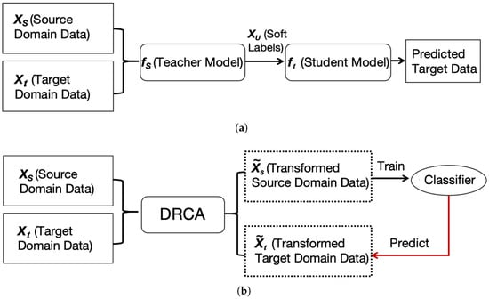
Figure 1.
Pipeline of KD and DRCA for drift compensation: (a) training a teacher model on the source domain to generate soft labels, which supervise the student model; (b) DRCA maps the source and target domain data into a shared domain-invariant feature subspace. The transformed source data is used to learn a predictor for the transformed target domain data.
2.2.1. Training the Teacher Model Using Source Domain Data
Consider a set of annotated samples from a source domain , where represents a d-dimensional feature and is its corresponding label in one-hot coding. Assuming there is a set that holds functions , we first aim to learn a feature representation (teacher model) via the minimization of a cross-entropy loss function, l, according to Equation (1) [26]:
Similar to standard supervised learning, the teacher network is optimized using the cross-entropy loss function.
2.2.2. Training the Student Model for the Target Domain
Even if is suitable for classifying the observations from the source domain , it may not be suitable for data coming from a different testing distribution (target domain ). We aim to find another function , which is suitable for classifying data from . Assuming we have access to a limited set of unlabeled samples in the target domain (where denotes the number of target domain samples), we can create a set
that is used to optimize a student model using the distillation loss. Through soft labels of this union , the student is expected to learn a better mapping to the labels than the teacher network by mitigating the overfitting to the source domain data [26]. When training the student network, we consider probability distributions over the labels as targets. This representation reflects the uncertainty of the prediction by the teacher network. The function is found by (approximately) solving,
Here, is the temperature parameter that controls the smoothness of the class probability prediction given by . The student minimizes the divergence to the teacher’s soft distributions for source and target samples, as in Equation (4), without additional task-specific losses. Because soft labels cover both domains, the student acquires target domain distributional information while maintaining dependence on source domain regularities and label supervision, which helps avoid catastrophic forgetting. Compared with hard-label supervision, soft targets provide fine-grained signals that more robustly convey class boundary information under domain shift [34]. We keep the rest of the training setup the same as the baseline (optimizer, schedule, etc.) to isolate the effect of KD for sensor-drift compensation; samples from both domains are randomly interleaved before forming mixed-ratio mini-batches. The exact T is selected via hyperparameter tuning on the target domain validation split.
2.2.3. Hyperparameter Selection
Two KD-specific hyperparameters are critical in our setting: the temperature T, used to generate the teacher’s soft targets, and the source/target data ratio, used when constructing mini-batches for student training.
Temperature . In Equation (4), the teacher logits are scaled by T before the softmax operation, i.e., . A larger T yields a softer probability distribution (higher entropy) that emphasizes inter-class similarity and provides smoother gradients, which can improve generalization under domain shift; in contrast, a smaller T yields a sharper distribution closer to hard labels, which may preserve discriminative information but can also increase the risk of overfitting to the source domain supervision. To account for both regimes, we consider a broad candidate set of T values (Section 2.5) and select T via validation-based selection for each task/target batch. Specifically, T is chosen to maximize the validation accuracy on the target domain validation split, and the selected T is then fixed when reporting results on the corresponding test split (repeated over 30 random partitions).
Source/target data ratio. When training the student, we interleave source and target samples within each mini-batch to stabilize learning signals from both domains. Unless otherwise stated, we use an approximately balanced ratio (about 1:1) by sampling an equal number of source domain () and target domain () instances per mini-batch. This design prevents the student from being dominated by either domain and keeps the optimization of Equation (4) numerically stable across tasks.
2.3. Domain-Regularized Component Analysis
As shown in the conceptual diagram in Figure 1b, Domain-Regularized Component Analysis (DRCA) projects source and target samples into a shared low-dimensional subspace, where inter-domain differences are compressed while intra-domain structures are preserved. We use DRCA as a feature-alignment step, following prior benchmarking on the same dataset [23]: first align features between the source and target domains, then train the downstream predictor on the aligned representation to improve target domain classification performance [23,24,25].
Domain-Regularized Component Analysis (DRCA) [23,24], a representative domain adaptation approach from a data perspective, transforms features into a subspace through a linear projection that minimizes scatter between the source and target domains while preserving within-domain scatter. Specifically, DRCA [23] projects features onto a hyperplane that minimizes scatter between the source and target domains after projection. Let the data in the source domain be denoted as , where , and represents the number of samples in the source domain. Similarly, samples in the target domain are denoted as , where , and D denotes the dimension of the original feature space [25]. Summary statistics of the data distribution in the original feature space include the following:
- (a)
- Mean of source domain measurements:Mean of target domain measurements:and overall mean:
- (b)
- Within-domain scatter for source and target domains:
- (c)
- Between-domain scatter:
The optimization objective of DRCA is to find a projection matrix that minimizes between-domain scatter while maintaining within-domain scatter on the projected hyperplane [23,25]. Here, d is the dimension of the new feature space after projection. For a measurement projected to , where , summary statistics on the projected space include the following: 1. Within-domain scatter for projected source and target domain measurements: and . 2. Between-domain scatter on the projection hyperplane: . The problem is formulated to maximize
where is a hyperparameter. By introducing a Lagrangian multiplier, the Lagrangian is expressed as
where is the Lagrange multiplier and is a constant. Taking the derivative with respect to P and setting it to zero transforms the problem into an eigenvalue decomposition [23,24,25]:
Sorting eigenvectors by eigenvalues, the top d eigenvectors form the projection matrix. This projects data from and to and . The projection dimension d and the target domain weight are chosen through hyperparameter tuning that (i) balances the weights on the source and target domain data, and (ii) favors combinations that yield stable downstream classification and a smaller projected between-domain term. This avoids excessive noise from overly large d and loss of discriminative variance from overly small d [25].
As a result, our final DRCA pipeline can be summarized as follows: (1) estimate statistics on the source domain and the target domain to learn the DRCA projection matrix ; (2) project both domains into the learned low-dimensional subspace; (3) train the downstream predictor only on projected source samples; (4) at inference, apply the trained predictor to projected target samples; and (5) keep the downstream classification model structure and hyperparameters consistent with the baseline (except input dimension after projection) so improvements can be attributed to DRCA itself [25]. Here, P is the linear projection matrix learned by DRCA that maps the original D-dimensional feature vector x to a d-dimensional subspace via , where z is used for downstream classification.
2.4. Hybrid Method: KD–DRCA
To address the limitations of existing methods and improve the effectiveness of domain adaptation, we integrated DRCA with KD, two domain adaptation approaches from different perspectives. First, we used DRCA to project the data onto a feature subspace to mitigate differences between the target and source domains. Subsequently, we used KD to train a teacher model and a student model on the projected data. After domain alignment via DRCA, KD transfers knowledge from the teacher model to the student model. We validated the effectiveness of the proposed method through a series of experiments.
2.5. Model Development and Evaluation
A Fully Connected Neural Network (FCNN) with four layers was used for all prediction tasks. The hidden units were [100, 50, 20], with rectified linear unit (ReLU) activation and a final softmax output layer for 6 classes. This architecture was first optimized under within-batch classification using a 70%/15%/15% train/validation/test split, and we used the same architecture for all cross-domain experiments to ensure fair comparison.
For the two cross-domain prediction tasks, we randomly partitioned the target batch into 50% validation and 50% test data. To account for randomness and evaluate robustness, we repeated this random partitioning 30 times (with different random seeds) and reported the distribution and statistics of the results across the 30 runs.
We tuned the key hyperparameters via validation-based grid search, including the KD temperature , the DRCA subspace dimensionality , and the DRCA target domain weight . These ranges were chosen to cover both sharp (low T) and soft (high T) teacher distributions and to span multiple orders of magnitude for , since the optimal target domain weighting is data-dependent. For each task/target batch, we selected hyperparameters by maximizing the mean validation accuracy over the 30 random 50%/50% target validation/test splits. On the validation and test sets, we evaluated performance using four metrics: accuracy, F1 score, recall, and precision. The within-batch classification performance was also reported as the ideal performance without domain drift.
We tuned the KD temperature T for each target batch by selecting the value that maximized the mean validation accuracy over 30 random 50%/50% validation/test splits (Table 1). Since a larger T yields a softer teacher distribution while a smaller T produces a sharper one, we further performed a sensitivity analysis on a representative task (Task 2: train on Batches 1–9 → test on Batch 10) by sweeping T over the same range; Figure S1 reports the mean ± std test accuracy across 30 splits, indicating that performance was relatively stable around the selected temperature.

Table 1.
KD temperature T selected for each target batch in Task 1 and Task 2 (chosen through validation-based grid search to maximize mean validation accuracy over 30 random validation/test splits).
2.6. Statistical Test
To test whether there were statistically significant differences between methods, paired t-tests were conducted on the results of 30 parallel experiments.
3. Results
3.1. Data Visualization Under Sensor Drift
The feature-space data distribution of the ten batches is visualized in Figure 2. The results show that clusters of different classes drifted in the feature space across the batches, illustrating the effect of sensor drift across data collection times.
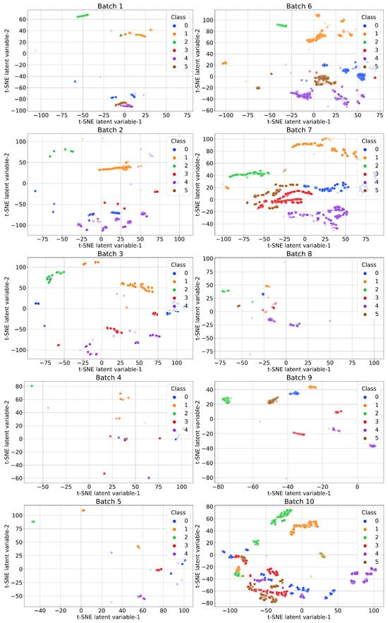
Figure 2.
Visualization of sensor drift in the feature space of the ten batches of data with t-SNE. Classes: 0—ethanol; 1—ethylene; 2—ammonia; 3—acetaldehyde; 4—acetone; 5—toluene.
3.2. Performance of Drift Compensation Methods
With hyperparameters tuned, classification performance on the test sets is presented in Figure 3. It should be noted that drift compensation does not guarantee improvements for every metric at every drift stage (target batch), and some methods may underperform compared to the baseline on specific batches or metrics. To make the comparison clearer, we additionally report the relative change (Δ%) with respect to the baseline (computed from the mean over 30 splits) in Figures S2 and S3, and summarize the overall trends and significance in Figure 4 and Table 2 and Table 3. It can be observed that on the test sets across the batches, KD consistently outperformed the baseline, DRCA, and KD–DRCA methods in most cases. In Task 1, over time (from Batch 2 to Batch 10), overall classification performance with Batch 1 as the source domain and any other batch as the target domain decreased, demonstrating the gradually worsening sensor drift. The results on the validation sets are shown in Figure S4. Beyond mean performance, Figure 3 visualizes the run-to-run variability across the 30 random target splits. Overall, KD tended to produce a more compact distribution (smaller interquartile range and fewer extreme outliers) than DRCA and KD–DRCA, suggesting more stable adaptation under drift. In contrast, DRCA (and KD–DRCA in some batches) showed a larger spread and occasional low-performance outliers, which can be attributed to the sensitivity of the learned projection to the specific target split and to increased drift severity in later batches. This further motivated our use of repeated experiments and statistical tests rather than single-run reporting. For most experiments, there was at least one drift compensation method that outperformed the baseline. As a reference for ideal classification performance without any sensor drift, the mean and standard deviation of the classification accuracy, F1-score, recall, and precision across 10 within-batch classification tasks were 0.979 (0.035), 0.978 (0.039), 0.979 (0.035), and 0.981 (0.037). It can be seen that under sensor drift, performance was generally worse than that on the within-batch classification tasks. As a summary of cross-domain classification, Table 2 presents the statistical test results comparing all test experiments and metrics to the baseline. Table 3 presents the results on the test sets for Task 1 and Task 2 separately.
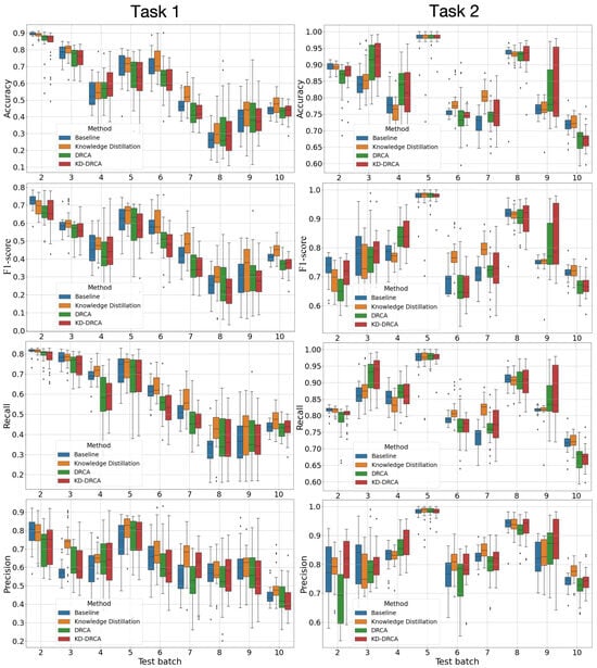
Figure 3.
Classification performance of the baseline, KD, DRCA, and KD–DRCA methods on the test sets of different data batches. Task 1: Train on the first batch and test on the remaining batches; Task 2: Train on all previous batches and test on the next batch.
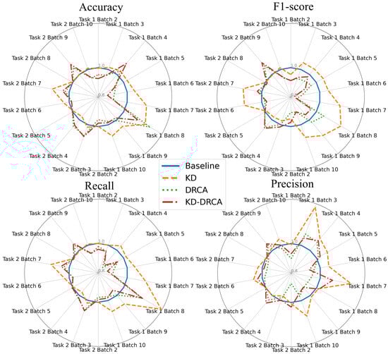
Figure 4.
Summary radar plots of the mean classification performance of different methods relative to the baseline across four metrics for all tasks on the test sets. The radar plots compare four methods—baseline, KD, DRCA, and KD–DRCA—across two tasks and nine target batches per task. Each axis represents a task–batch combination, with values showing the median performance across 30 parallel experiments (normalized to the baseline). Task 1: Train on the first batch and test on the remaining batches; Task 2: Train on all previous batches and test on the next batch.
Table 2.
Counts of statistically significant differences compared with the baseline. Each method has 72 samples: two cross-domain tasks, nine target batches per task, and four metrics. Values in parentheses are the results on the validation sets.
Table 3.
Counts of statistically significant differences on the test sets for Task 1 (left of “/”) and Task 2 (right of “/”) compared with the baseline.
Unless otherwise stated, we report the mean ± standard deviation across 30 random 50%/50% validation/test splits. The relative improvement over the baseline was computed as , where denotes the mean performance across the 30 splits. Across all cross-domain tasks and target batches, the maximum relative improvement in accuracy was 18%, and the maximum relative improvement in the macro-F1-score was 15%.
Table 2 shows that both KD and KD–DRCA resulted in more statistically significant improvements () than DRCA, while KD yielded the fewest statistically significant decreases (). Table 3 shows that KD was the best method, with DRCA and KD–DRCA performing better in Task 2 than in Task 1.
The radar plots in Figure 4 show the mean test-set performance across metrics, batches, and tasks. Figure S5 shows the validation results, while Figure S6 and Figure S7 present the median values on the test and validation sets, respectively.
Overall, KD achieved more frequent and larger performance gains and significantly outperformed the previously validated DRCA method [23]. We further evaluated an exploratory hybrid KD–DRCA approach motivated by potential complementarity between DRCA’s subspace alignment and KD’s soft-target regularization; however, KD–DRCA was not consistently better than KD alone. Therefore, KD remains the most suitable choice for electronic-nose drift compensation in our setting.
4. Discussion
This study systematically evaluated the effectiveness of the KD and DRCA methods, and their combination, to address sensor drift in electronic-nose-based gas classification, a field in which accurate gas classification is critical but often challenged by drift [30]. Although prior studies have confirmed the effectiveness of certain methods on this public dataset, they often relied on single-run evaluations and lacked statistical rigor. The primary contribution of this study lies in the design of a statistically validated experimental setup with robust cross-domain testing. This setup addresses gaps in prior studies, which often lacked randomization and rigorous statistical validation. Additionally, we implemented a teacher–student knowledge distillation (KD) framework as a model-level drift compensation strategy and evaluated it under long-term temporal drift through repeated randomized trials and statistical significance testing on the UCI drift benchmark, using the previously validated DRCA as a benchmark for comparison [23]. Importantly, in the systematic and statistical validation, KD achieved the best performance for electronic-nose drift compensation, marking a significant advancement in this research area.
Although previous studies, such as Zhang et al. [23], have applied DRCA, their evaluation setting differed from a more deployment-like scenario in two key aspects: (1) they mainly evaluated DRCA using consecutive-batch transfers (e.g., train on Batch 2 → test on Batch 3, and Batch 3 → Batch 4), whereas in real-world scenarios, models are typically trained on all prior data (e.g., Batches 1–4) and then used to predict unseen new data (e.g., Batch 5) [35]; and (2) the reported results were largely based on single-run/single-split evaluations without repeated trials and statistical significance testing. This more realistic drift compensation setting is likely more challenging because combining all previous data batches can introduce heterogeneous domain differences, making prediction more difficult than transfer between single batches. Therefore, it is important to evaluate DRCA under more realistic settings with rigorous statistical testing. Our study sought to fill these gaps by testing these methods across multiple cross-domain prediction tasks with repeated random splits and statistical significance tests.
Additionally, we explored a combined approach using KD and DRCA. The hybrid KD–DRCA method aimed to leverage the complementary strengths of data-level and model-level strategies: DRCA was used to minimize domain differences [24], and KD was employed to enhance model generalization by transferring knowledge from a complex teacher model to a simpler student model [36]. However, the results indicated that KD alone outperformed both DRCA and the KD–DRCA hybrid, making it the most suitable method for mitigating sensor drift in gas sensor applications. We further analyzed the underlying reasons why KD consistently outperformed DRCA in our experiments. First, KD leverages soft targets produced by the teacher model, which encode inter-class similarity information rather than only hard one-hot labels. Such soft supervision acts as an implicit regularizer, reducing overfitting to source domain noise and encouraging smoother decision boundaries that generalize better under drift. Second, the student model in KD learns a non-linear mapping that matches the teacher’s probability structure across both source and target samples, which can better preserve class-separation information under complex drift patterns. In contrast, DRCA relies on a linear subspace projection to compress domain discrepancy, which may inadvertently discard discriminative variance when the drift is non-linear or heterogeneous across batches. Therefore, KD can preserve more stable decision boundaries across domains, achieving stronger performance in our cross-domain evaluation. This finding highlights KD’s effectiveness in scenarios in which sensor drift is not as pronounced, as its semi-supervised nature appears to be more adept at handling the nuances of the drift problem [37].
Despite the overall positive results achieved by KD, no drift compensation method is guaranteed to improve performance under sensor drift in all experiments, which highlights the need for better control in electronic-nose deployment in addition to drift compensation. Despite the promising results, there are limitations to this study. Our study did not include a comparison with more complicated methods such as CycleGAN [38] or reliability-based semi-supervised learning approaches [27] that have shown promise in drift compensation. Future research may benefit from incorporating these methods for a more comprehensive evaluation. We acknowledge that the UCI Gas Sensor Array Drift Dataset mainly reflects long-term temporal drift in a fixed experimental setup, and it does not allow us to disentangle temporal drift from other real-world sources of drift such as environmental or operational changes (e.g., humidity/temperature shifts) or sensing material deterioration/poisoning. While KD and DRCA are data-driven and could, in principle, be applied to these broader drift scenarios given representative target domain samples, their effectiveness under cross-environment deployment shifts requires dedicated validation on datasets explicitly covering such factors (e.g., models developed in cold/dry conditions and deployed in hot/humid conditions). We therefore leave cross-environment and multi-factor drift compensation as an important direction for future work. Furthermore, the current study was limited to a single dataset. Therefore, in the future, validating the findings on other datasets could strengthen the generalizability of the results.
5. Conclusions
This study introduced and validated knowledge distillation (KD) as an effective approach for mitigating sensor drift in electronic-nose-based gas recognition. Across extensive cross-domain experiments, KD consistently outperformed Domain-Regularized Component Analysis (DRCA) and the hybrid KD–DRCA, improving accuracy, precision, recall, and F1-score. This represents the first demonstration of semi-supervised KD for sensor-drift compensation, offering a statistically robust foundation for future real-world applications. Future work will extend validation to additional datasets and explore integration with more advanced semi-supervised and generative adaptation techniques.
Supplementary Materials
The following supporting information can be downloaded at https://www.mdpi.com/article/10.3390/informatics13010015/s1: Figure S1: KD temperature sensitivity on a representative cross-domain task; Figure S2: Relative performance change (Δ%) with respect to the baseline on the test sets; Figure S3: Relative performance change (Δ%) with respect to the baseline on the validation sets; Figure S4: Classification performance of baseline, KD, DRCA, and KD-DRCA methods on the test sets across different batches; Figure S5: Mean radar plots of relative classification performance across four metrics on the validation sets; Figure S6: Median radar plots of relative classification performance across four metrics on the test sets; Figure S7: Median radar plots of relative classification performance across four metrics on the validation sets.
Author Contributions
Conceptualization, J.L. and X.Z.; methodology, J.L. and X.Z.; software, J.L.; validation, J.L. and X.Z.; formal analysis, J.L.; investigation, J.L.; resources, X.Z.; data curation, J.L.; writing—original draft preparation, J.L.; writing—review and editing, X.Z.; visualization, J.L.; supervision, X.Z.; project administration, X.Z. All authors have read and agreed to the published version of the manuscript.
Funding
This research received no external funding.
Institutional Review Board Statement
Not applicable.
Informed Consent Statement
Not applicable.
Data Availability Statement
Publicly available datasets were used in this study. The UCI Gas Sensor Array Drift Dataset is available at http://archive.ics.uci.edu/ml/datasets/Gas+Sensor+Array+Drift+Dataset (accessed on 7 November 2024). The code to reproduce the experiments and figures is available at https://github.com/abob7/gas-drift (accessed on 7 November 2024).
Acknowledgments
We acknowledge the University of California, Irvine (UCI) Machine Learning Repository for providing the dataset.
Conflicts of Interest
The authors declare no conflicts of interest.
References
- Bhattacharyya, N.; Bandyopadhyay, R.; Bhuyan, M.; Tudu, B.; Ghosh, D.; Jana, A. Electronic nose for black tea classification and correlation of measurements with “Tea Taster” marks. IEEE Trans. Instrum. Meas. 2008, 57, 1313–1321. [Google Scholar] [CrossRef]
- Sarkodie, K.; Fergusson-Rees, A.; Diaz, P. A review of the application of non-intrusive infrared sensing for gas–liquid flow characterization. J. Comput. Multiph. Flows 2018, 10, 43–56. [Google Scholar] [CrossRef]
- Wang, Y.; Wang, Z.; Diao, J.; Sun, X.; Luo, Z.; Li, G. Discrimination of different species of dendrobium with an electronic nose using aggregated conformal predictor. Sensors 2019, 19, 964. [Google Scholar] [CrossRef]
- Borowik, P.; Adamowicz, L.; Tarakowski, R.; Wacławik, P.; Oszako, T.; Ślusarski, S.; Tkaczyk, M. Application of a low-cost electronic nose for differentiation between pathogenic oomycetes pythium intermedium and phytophthora plurivora. Sensors 2021, 21, 1326. [Google Scholar] [CrossRef] [PubMed]
- Flammini, A.; Marioli, D.; Taroni, A. A low-cost interface to high-value resistive sensors varying over a wide range. IEEE Trans. Instrum. Meas. 2004, 53, 1052–1056. [Google Scholar] [CrossRef]
- Pace, C.; Fragomeni, L.; Khalaf, W. Developments and applications of electronic nose systems for gas mixtures classification and concentration estimation. In Applications in Electronics Pervading Industry, Environment and Society: APPLEPIES 2014; Springer International Publishing: Cham, Switzerland, 2016; pp. 1–7. [Google Scholar]
- De Vito, S.; Piga, M.; Martinotto, L.; Di Francia, G. CO, NO2 and NOx urban pollution monitoring with on-field calibrated electronic nose by automatic bayesian regularization. Sens. Actuators B Chem. 2009, 143, 182–191. [Google Scholar] [CrossRef]
- Musatov, V.Y.; Sysoev, V.; Sommer, M.; Kiselev, I. Assessment of meat freshness with metal oxide sensor microarray electronic nose: A practical approach. Sens. Actuators B Chem. 2010, 144, 99–103. [Google Scholar] [CrossRef]
- Wojnowski, W.; Majchrzak, T.; Dymerski, T.; Gębicki, J.; Namieśnik, J. Portable electronic nose based on electrochemical sensors for food quality assessment. Sensors 2017, 17, 2715. [Google Scholar] [CrossRef]
- Loutfi, A.; Coradeschi, S.; Mani, G.K.; Shankar, P.; Rayappan, J.B.B. Electronic noses for food quality: A review. J. Food Eng. 2015, 144, 103–111. [Google Scholar] [CrossRef]
- Rodríguez, J.; Durán, C.; Reyes, A. Electronic nose for quality control of Colombian coffee through the detection of defects in “Cup Tests”. Sensors 2009, 10, 36–46. [Google Scholar] [CrossRef]
- Miao, J.; Luo, Z.; Wang, Y.; Li, G. Comparison and data fusion of an electronic nose and near-infrared reflectance spectroscopy for the discrimination of ginsengs. Anal. Methods 2016, 8, 1265–1273. [Google Scholar] [CrossRef]
- Zhan, X.; Guan, X.; Wu, R.; Wang, Z.; Wang, Y.; Li, G. Feature engineering in discrimination of herbal medicines from different geographical origins with electronic nose. In Proceedings of the 2019 IEEE 7th International Conference on Bioinformatics and Computational Biology (ICBCB); IEEE: Piscataway, NJ, USA, 2019; pp. 56–62. [Google Scholar]
- Schmekel, B.; Winquist, F.; Vikström, A. Analysis of breath samples for lung cancer survival. Anal. Chim. Acta 2014, 840, 82–86. [Google Scholar] [CrossRef]
- Zhan, X.; Wang, Z.; Yang, M.; Luo, Z.; Wang, Y.; Li, G. An electronic nose-based assistive diagnostic prototype for lung cancer detection with conformal prediction. Measurement 2020, 158, 107588. [Google Scholar] [CrossRef]
- Rodriguez-Lujan, I.; Fonollosa, J.; Vergara, A.; Homer, M.; Huerta, R. On the calibration of sensor arrays for pattern recognition using the minimal number of experiments. Chemom. Intell. Lab. Syst. 2014, 130, 123–134. [Google Scholar] [CrossRef]
- Jha, S.K.; Hayashi, K.; Yadava, R. Neural, fuzzy and neuro-fuzzy approach for concentration estimation of volatile organic compounds by surface acoustic wave sensor array. Measurement 2014, 55, 186–195. [Google Scholar] [CrossRef]
- Zhan, X.; Guan, X.; Wu, R.; Wang, Z.; Wang, Y.; Luo, Z.; Li, G. Online conformal prediction for classifying different types of herbal medicines with electronic nose. In IET Doctoral Forum on Biomedical Engineering, Healthcare, Robotics and Artificial Intelligence 2018 (BRAIN 2018); IET: Stevenage, UK, 2018. [Google Scholar]
- Yang, S.; Zhang, H.; Li, Z.; Duan, S.; Yan, J. Identification of industrial exhaust based on an electronic nose with an interleaved grouped residual convolutional compression network. Sens. Actuators A Phys. 2023, 363, 114692. [Google Scholar] [CrossRef]
- Hossein-Babaei, F.; Ghafarinia, V. Compensation for the drift-like terms caused by environmental fluctuations in the responses of chemoresistive gas sensors. Sens. Actuators B Chem. 2010, 143, 641–648. [Google Scholar] [CrossRef]
- Zhang, L.; Tian, F.; Liu, S.; Dang, L.; Peng, X.; Yin, X. Chaotic time series prediction of E-nose sensor drift in embedded phase space. Sens. Actuators B Chem. 2013, 182, 71–79. [Google Scholar] [CrossRef]
- Zhan, X.; Liu, Y.; Cecchi, N.J.; Gevaert, O.; Zeineh, M.M.; Grant, G.A.; Camarillo, D.B. Brain deformation estimation with transfer learning for head impact datasets across impact types. IEEE Trans. Biomed. Eng. 2024, 71, 1853–1863. [Google Scholar] [CrossRef]
- Zhang, L.; Liu, Y.; He, Z.; Liu, J.; Deng, P.; Zhou, X. Anti-drift in E-nose: A subspace projection approach with drift reduction. Sens. Actuators B Chem. 2017, 253, 407–417. [Google Scholar] [CrossRef]
- Wang, H.; Zhan, X.; Liu, L.; Ullah, A.; Li, H.; Gao, H.; Wang, Y.; Hu, R.; Li, G. Unsupervised cross-user adaptation in taste sensation recognition based on surface electromyography. IEEE Trans. Instrum. Meas. 2022, 71, 1–11. [Google Scholar] [CrossRef]
- Zhan, X.; Sun, J.; Liu, Y.; Cecchi, N.J.; Le Flao, E.; Gevaert, O.; Zeineh, M.M.; Camarillo, D.B. Adaptive machine learning head model across different head impact types using unsupervised domain adaptation and generative adversarial networks. IEEE Sens. J. 2024, 24, 7097–7106. [Google Scholar] [CrossRef]
- Orbes-Arteainst, M.; Cardoso, J.; Sørensen, L.; Igel, C.; Ourselin, S.; Modat, M.; Nielsen, M.; Pai, A. Knowledge distillation for semi-supervised domain adaptation. In Proceedings of the OR 2.0 Context-Aware Operating Theaters and Machine Learning in Clinical Neuroimaging: Second International Workshop, OR 2.0 2019, and Second International Workshop, MLCN 2019, Held in Conjunction with MICCAI 2019, Shenzhen, China, 13 and 17 October 2019; Proceedings 2; Springer: Cham, Switzerland, 2019; pp. 68–76. [Google Scholar]
- Liu, L.; Zhan, X.; Wu, R.; Guan, X.; Wang, Z.; Zhang, W.; Pilanci, M.; Wang, Y.; Luo, Z.; Li, G. Boost AI power: Data augmentation strategies with unlabeled data and conformal prediction, a case in alternative herbal medicine discrimination with electronic nose. IEEE Sens. J. 2021, 21, 22995–23005. [Google Scholar] [CrossRef]
- Liu, L.; Zhan, X.; Yang, X.; Guan, X.; Wu, R.; Wang, Z.; Luo, Z.; Wang, Y.; Li, G. Cpsc: Conformal prediction with shrunken centroids for efficient prediction reliability quantification and data augmentation, a case in alternative herbal medicine classification with electronic nose. IEEE Trans. Instrum. Meas. 2022, 71, 1–11. [Google Scholar] [CrossRef]
- Vergara, A. Gas Sensor Array Drift Dataset. UCI Machine Learning Repository. 2012. Available online: https://archive.ics.uci.edu/ml/datasets/Gas+Sensor+Array+Drift+Dataset (accessed on 7 November 2024).
- Vergara, A.; Vembu, S.; Ayhan, T.; Ryan, M.A.; Homer, M.L.; Huerta, R. Chemical gas sensor drift compensation using classifier ensembles. Sens. Actuators B Chem. 2012, 166, 320–329. [Google Scholar] [CrossRef]
- Chang, I.S.; Byun, S.W.; Lim, T.B.; Park, G.M. A study of drift effect in a popular metal oxide sensor and gas recognition using public gas datasets. IEEE Access 2023, 11, 26383–26392. [Google Scholar] [CrossRef]
- Dennler, N.; Rastogi, S.; Fonollosa, J.; Van Schaik, A.; Schmuker, M. Drift in a popular metal oxide sensor dataset reveals limitations for gas classification benchmarks. Sens. Actuators B Chem. 2022, 361, 131668. [Google Scholar] [CrossRef]
- Rehman, A.U.; Belhaouari, S.B.; Ijaz, M.; Bermak, A.; Hamdi, M. Multi-classifier tree with transient features for drift compensation in electronic nose. IEEE Sens. J. 2020, 21, 6564–6574. [Google Scholar] [CrossRef]
- Hinton, G.; Vinyals, O.; Dean, J. Distilling the knowledge in a neural network. arXiv 2015, arXiv:1503.02531. [Google Scholar] [CrossRef]
- Liang, J.; Jiang, L.; Hauptmann, A.G. SimAug: Learning Robust Representations from Simulation for Trajectory Prediction. In Proceedings of the Computer Vision–ECCV 2020; Vedaldi, A., Bischof, H., Brox, T., Frahm, J.M., Eds.; Lecture Notes in Computer Science; Springer: Cham, Switzerland, 2020; Volume 12358, pp. 275–292. [Google Scholar] [CrossRef]
- Abbasi, S.; Hajabdollahi, M.; Karimi, N.; Samavi, S. Modeling teacher-student techniques in deep neural networks for knowledge distillation. In Proceedings of the 2020 International Conference on Machine Vision and Image Processing (MVIP); IEEE: Piscataway, NJ, USA, 2020; pp. 1–6. [Google Scholar]
- Gomes, H.M.; Grzenda, M.; Mello, R.; Read, J.; Le Nguyen, M.H.; Bifet, A. A survey on semi-supervised learning for delayed partially labelled data streams. ACM Comput. Surv. 2022, 55, 1–42. [Google Scholar] [CrossRef]
- Zhu, J.Y.; Park, T.; Isola, P.; Efros, A.A. Unpaired image-to-image translation using cycle-consistent adversarial networks. In Proceedings of the IEEE International Conference on Computer Vision, Venice, Italy, 22–29 October 2017; pp. 2223–2232. [Google Scholar]


Disclaimer/Publisher’s Note: The statements, opinions and data contained in all publications are solely those of the individual author(s) and contributor(s) and not of MDPI and/or the editor(s). MDPI and/or the editor(s) disclaim responsibility for any injury to people or property resulting from any ideas, methods, instructions or products referred to in the content. |
© 2026 by the authors. Licensee MDPI, Basel, Switzerland. This article is an open access article distributed under the terms and conditions of the Creative Commons Attribution (CC BY) license.