Claim Watching and Individual Claims Reserving Using Classification and Regression Trees

Abstract

We present an approach to individual claims reserving and claim watching in general insurance based on classification and regression trees (CART). We propose a compound model consisting of a frequency section, for the prediction of events concerning reported claims, and a severity section, for the prediction of paid and reserved amounts. The formal structure of the model is based on a set of probabilistic assumptions which allow the provision of sound statistical meaning to the results provided by the CART algorithms. The multiperiod predictions required for claims reserving estimations are obtained by compounding one-period predictions through a simulation procedure. The resulting dynamic model allows the joint modeling of the case reserves, which usually yields useful predictive information. The model also allows predictions under a double-claim regime, i.e., when two different types of compensation can be required by the same claim. Several explicit numerical examples are provided using motor insurance data. For a large claims portfolio we derive an aggregate reserve estimate obtained as the sum of individual reserve estimates and we compare the result with the classical chain-ladder estimate. Backtesting exercises are also proposed concerning event predictions and claim-reserve estimates.

1. Introduction

In the settlement process of a general insurance claims portfolio we denote as claim watching the insurer’s activityconsisting of monitoring and controlling the cost development at single-claim level. Claim watching encompasses prediction of specific events regarding individual claims that can be relevant for cost development and could be influenced by possible appropriate management actions. Obviously, the estimation of the ultimate cost, hence the individual claims reserving, is also a typical claim watching activity. Early-warning systems at single-claim or group-of-claims level can be also included.

In this paper, we propose a machine-learning approach to claim watching, and individual claims reserving, using a prediction model based on the classification and regression trees (CART). The paper is largely based on a path-breaking article produced in 2016 by Mario Wüthrich (Wüthrich 2016) where individual claims reserving is addressed by CART techniques. The method proposed by Wüthrich was restricted “for pedagogical reasons” to the prediction of events and the estimation of the number of payments related to individual claims. We extend Wüthrich’s paper providing a so-called frequency-severity model where claim amounts paid are also considered. Moreover, we enlarge the set of the response and explanatory variables of the model to allow prediction under a double-claim regime, i.e., when two different types of compensation can be required by the same claim. This multi-regime extension enables us to provide meaningful applications to Italian motor insurance claims data. We also propose a further enhancement of the CART approach allowing the joint dynamic modeling of the case reserves, which usually yield useful predictive information.

The claim watching idea and a related frequency-severity model based on CARTs were introduced and developed in D’Agostino et al. (2018) and large part of the material presented here was already contained in that paper.

According to a point of view proposed in Hiabu et al. (2015), a possible inclusion of a granular data approach in claims reserving could be provided by extending classical aggregate methods, adding more model structure to include underlying effects which are supposed to emerge at an individual claim level. In Hiabu et al. (2015) this approach is illustrated by referring to a series of extensions of the Double Chain-Ladder (DCL) model, originated in Verral et al. (2010) and developed in successive papers, (see e.g., Martínez-Miranda et al. 2011, 2012, 2013). Approaches to claims reserving recently proposed based on embedding a classical actuarial model in a neural net (see e.g., Gabrielli et al. 2018; Wüthrich and Merz 2019) could also be interpreted as going in a similar “top-down” direction. A different path is followed in this paper. We use the large model flexibility provided by machine-learning methods for directly modeling individual claim histories. In this approach model assumptions are specified at granular level and are, in some sense, the minimal required to guarantee a sound statistical meaning to results provided by the powerful algorithms currently available. This allows implantation of claim watching activities which can be considered even more general than traditional claims reserving.

This paper, however, has several limitations. In particular, only point estimates of the ultimate claim cost are considered and the important problem of prediction uncertainty is not addressed, yet. Moreover, these cost estimates do not fully include underwriting year inflation, then an appropriate model should be added to this aim. Therefore, the present paper should be considered to be only a starting point in applying CARTs to claims reserving and claims handling. By analogy, one could say that in introducing machine learning to individual reserving data this paper is playing the same role as Verral et al. (2010) was playing in DCL: many improvements and developments should follow.

The present paper is composed of two parts. In the first part one-period prediction problems are considered. Prediction problems typical in claim watching and individual claims reserving are presented in Section 2 and notation and a basic assumption (i.e., the dependence of the prediction functions on the observation time-lag) are introduced in Section 3. In Section 4 we describe the general structure of the frequency-severity approach, providing details on the model assumptions for both the model components. The structure of the feature space, both for static and dynamic variables, is described in Section 5 and the organization of data required for the CART calibrations is illustrated in Section 6. In Section 7 the use of classification trees for the frequency prediction, and regression trees for (conditional) severity predictions is illustrated. In Section 8 a first extensive example of one-year predictions for a claims portfolio in Italian motor insurance is presented using the rpart routine implemented in R. The results of the CART calibration are discussed in detail and a possible use of event predictions for early warning is illustrated.

The second part of the paper considers multiperiod predictions and includes numerical examples and backtesting exercises. In Section 9 we consider multiperiod predictions and describe the properties required for deriving multiyear forecasts by compounding one-year forecasts. In Section 10 a simulation approach to multiperiod forecasts is also presented and additional assumptions allowing the joint dynamic modeling of the case reserves are discussed. A first numerical example of multiperiod prediction of a single-claim cost is also provided. Section 11 is devoted to numerical examples of applications to a large claims portfolio in motor insurance and to some backtesting exercises providing insights into the predictive performance of our CART approach. We first illustrate backtesting results for predictions of one-year event occurrences useful for claim watching. Finally, a typical claim reserving exercise is provided, composed of two steps. In a first step the individual reserve estimate is derived by simulation for all the claims in the portfolio and the resulting total reserve, after the addition of an IBNYR (incurred but not yet reported) reserve estimate, is compared with the classical chain-ladder reserve, estimated on aggregate payments at portfolio level (an ancillary model for IBNYR reserves is outlined in Appendix A). Since we perform these estimates on data deprived of the last calendar year observations, we analyze the predictive accuracy of the CART approach with respect to the chain-ladder approach by comparing the realized aggregate payments in the “first next diagonal” with those predicted by the two methods. Some conclusions are presented in Section 12.

Part I. One-period Predictions

2. A First Look at the Problem and the Model

Let us consider the claim portfolio of a given line of business of a non-life insurer. We are interested in the individual claim settlement processes of this portfolio. For example, for a given claim $\mathcal{C}$ in the portfolio, we would like to answer questions like these:

(a)

What is the probability that $\mathcal{C}$ is closed in the next year?

(b)

What is the probability that a lawyer will be involved in the settlement of $\mathcal{C}$ in two years?

(c)

What is the expectation of a payment in respect of $\mathcal{C}$ in the next year?

(d)

What is the expectation of the total claim payments in respect of $\mathcal{C}$ until finalization?

In general, we will refer to the activity of dealing with this kind of questions as claim watching. In particular, question (b) could be relevant in a possible early-warning system, while questions as (c) and (d) are more concerned with individual claims reserving. The classical claims reserving, i.e., the estimation of the outstanding loss liabilities aggregate over the entire portfolio, could be obtained by summing all the individual claim reserves with some corrections due to non-modeled effects (typically, reserve for IBNYR claims).

For a specified claim $\mathcal{C}$ in the portfolio, a typical claim watching question at time t can be formulated as a prediction problem with the form:

$$\mathbb{E}\left[Y_{t+\tau }^{(\mathcal{C})}|{\mathcal{F}}_t\right]=\mu \left({\mathit{x}}_t^{(\mathcal{C})}\right),\tau >0,$$

(1)

where:

·

${\mathcal{F}}_t$ denotes the information available at time t,

·

the vector ${\mathit{x}}_t^{(\mathcal{C})}\in \mathcal{X}$ is the claim feature (also covariates, explanatory variables, independent variables, …), which is observed up to time t, i.e., is ${\mathcal{F}}_t$-measurable,

·

$\mu :\mathcal{X}\to \mathbb{R}$ is the prediction function,

·

$Y_{t+\tau }^{(\mathcal{C})}$ is the response variable (or dependent variable).

Referring to the previous examples, the response in (1) can be specified as follows:

(a)

$Y_{t+\tau }^{(\mathcal{C})}$ is the indicator function of the event {$\mathcal{C}$ is closed at time $t+\tau$} (with $\tau =1$),

(b)

$Y_{t+\tau }^{(\mathcal{C})}$ is the indicator function of {$\mathcal{C}$ will involve a lawyer by the time $t+\tau$} (with $\tau =2$),

(c)

$Y_{t+\tau }^{(\mathcal{C})}$ is the random variable denoting the amount paid in respect of $\mathcal{C}$ at time $t+\tau$ (with $\tau =1$),

(d)

$Y_{t+\tau }^{(\mathcal{C})}$ is the random variable denoting the cumulated paid amount in respect of $\mathcal{C}$ at time $t+\tau$ (with $\tau \to \infty$).

The response and the feature can be both quantitative or qualitative variables and we do not assume for the moment a particular structure for the prediction function $\mu$, which must be estimated from the data. Usually, the prediction model (1) is referred to as regression model if the response is a quantitative variable and classification model if the response is qualitative (categorical). The prediction function is named, accordingly, as regression or classifier function1.

Questions such as (a) and (b) involve prediction of events while questions such as (c) and (d) concern prediction of paid amounts. With some abuse of actuarial jargon, we will refer to a prediction model for event occurrences as a frequency model. Similarly, we will refer to a prediction model for paid amounts as a severity model. Then, altogether, we need a frequency-severity model. We will develop a frequency-severity model for claim watching with a conditional severity component that is the paid amounts are predicted conditionally on the payment is made. This is because the probability distribution of a paid amount, with a discrete mass in 0, is better modeled by separate recognition of the mass and the remainder of the distribution (assumed continuous).

Remark 1.

A model with such a structure can be also referred to as a cascaded model, see  Taylor (2019) for a discussion of this kind of models. This model structure also bears some resemblance to Double Chain-Ladder (DCL), see Martínez-Miranda et al. (2012). In DCL a micro-model of the claims generating process is first introduced to predict the reported number of claims. Future payments are then predicted through a delay function and a severity model. In DCL, however, individual information is assumed to be “(in practice often) unobservable” and the micro-model is only aimed to derive a suitable reserving model for aggregate data. In this paper, instead, extensive individual information is assumed to be always available and each individual claim is identifiable. Moreover, we are interested in both claim watching and individual claims reserving, aggregate reserving being a possible byproduct of the approach.

To deal with the prediction problems both in the frequency and the severity component we shall use the classification and regression trees (CART) techniques, namely classification trees for the frequency section and regression trees for the severity section. One of the main advantages of CART methods is the large modeling flexibility (for aggregate claims reserving methods with a good degree of model flexibility though not using machine learning, see e.g., Pešta and Okhrin 2014). Carts can deal with any sort of structured and unstructured information, an underlying structural form of the prediction function $\mu$ can be learned from the data, many explanatory variables can be used, both quantitative and qualitative and observed at different dates. Moreover, the interpretability of results is generally allowed. As methods for providing expectations, CARTs can also be referred to as prediction trees.

3. Notation and Basic Assumptions

The notation used in this paper is essentially the same as in Wüthrich (2016). For simplicity sake we model the claim settlement process using an annual time grid. If allowed by the available data, a discrete time grid with a shorter time step (semester, quarter, month, …) could be used.

Accident year. For a given line of business in non-life insurance, let us consider a claims portfolio containing observations at the current date on the claims occurred during the last I accident years (ay). The accident years are indexed as $i=1,\dots ,I$. Then we are at time (calendar year) $t=I$.

Reporting delay. For each accident year i, claims may have been observed with a reporting delay (rd) $j=0,1,\dots$. A claim with accident year i and reporting delay j will have reporting date $i+j$. As usual, we assume that there exists a maximum possible delay $J\ge 0$.

Claims identification. Each claim is identified by a claim code cc. For each block $(i,j)$ there are $N_{i,j}$ claims and we denote by $\nu =1,\dots ,N_{i,j}$ the index numbering the claims in block $(i,j)$; the $\nu$-th claim in $(i,j)$ is denoted by ${\mathcal{C}}_{i,j}^{(\nu )}$.

IBNYR claims. Because of the possible reporting delay, at a given date t we can have incurred but not yet reported (IBNYR) claims. Since there is a maximal delay J, at the current date the IBNYR claims are those with delay $j>(I-i)\wedge J$. The maximum observed reporting delay is $(I-1)\wedge J$.

Remark 2.

At time I, claims with $j\le I-i$ can be closed or reported but not settled (RBNS). We can estimate a reserve required for these claims. For the IBNYR reserve estimate a specific reserving model is needed (see Appendix A).

Predictions in the claim settlement process. For given $i,j,\nu$, the claim settlement process of ${\mathcal{C}}_{i,j}^{(\nu )}$ is defined on the calendar dates $i+j,i+j+1,i+j+2,\dots$. Let us denote by:

·

${\mathit{X}}_{i,j|k}^{(\nu )}$ a generic random variable, possibly multidimensional, involved in the claim settlement process of ${\mathcal{C}}_{i,j}^{(\nu )}$ and observed at time $t=i+j+k$, for $k\in {\mathbb{N}}_0$,

·

$\ell :=j+k=t-i$ the time-lag of ${\mathit{X}}_{i,j|k}^{(\nu )}$.

Using this notation, the prediction problem (1) for $\tau =1$ is reformulated as follows:

$$\mathbb{E}[{\mathit{Y}}_{\underset{datet+1}{\underbrace{i,j|t-(i+j)+1}}}^{(\nu )}|{\mathcal{F}}_{i+j+k}]=\mu ({\mathit{x}}_{\underset{datet}{\underbrace{i,j|t-(i+j)}}}^{(\nu )}),$$

(2)

where the claim feature ${\mathit{x}}_{i,j|t-(i+j)}^{(\nu )}\in \mathcal{X}$ is ${\mathcal{F}}_{i+j+k}$-measurable, $\mu :\mathcal{X}\to \mathbb{R}$, and the response is possibly multidimensional. In the rest of the paper the prediction function $\mu$ will refer solely to one-year forecast problems. Multiyear prediction problems will be treated compounding one-year predictions.

To give some statistical structure to the prediction model, we make the following basic assumption on the prediction function:

(H0)

At any date t the one-year prediction function $\mu \left({\mathit{x}}_{i,j|t-(i+j)}^{(\nu )}\right)$ depends only on the time-lag $\ell =t-i$. i.e.,:

$${\mu }_{t-i}:\mathcal{X}\to \mathbb{R},{\mathit{x}}_{i,j|t-(i+j)}^{(\nu )}\mapsto {\mu }_{t-i}\left({\mathit{x}}_{i,j|t-(i+j)}^{(\nu )}\right).$$

Then the ${\mu }_{t-i}$ function is independent of $\nu$ and is applied to all the features with the same time-lag $\ell =t-i$, providing the expectation of ${\mathit{Y}}_{i,j|t-(i+j)+1}^{(\nu )}$ (which has time-lag $\ell +1$).

Under assumption (H0) we can build statistical samples of observed pairs feature-response which can be used to derive an estimate of unobserved responses based on observed features.

In what follows it will be often convenient to rewrite the prediction problem using the k index. Since $t=i+j+k$ expression (2), taking account of assumption (H0), takes the form:

$$\mathbb{E}\left[{\mathit{Y}}_{i,j|k+1}^{(\nu )}|{\mathcal{F}}_{i+j+k}\right]={\mu }_{j+k}\left({\mathit{x}}_{i,j|k}^{(\nu )}\right).$$

(3)

4. The General Structure of the Frequency-Severity Model

To give a formal characterization of the entire claim settlement process we have to recall that $N_{i,j}$ denotes the number of claims occurred in accident year i reported in calendar year $i+j$. Then in a general setting we let the relevant indexes vary as follows:

$$i=1,\dots ,I,j=0,\dots ,J,\nu \in {\mathbb{N}}_1,k\in {\mathbb{N}}_0,$$

and we consider also $N_{i,j}$ as a stochastic process.

4.1. Frequency and Severity Response Variables

The peculiarity of the frequency model is that the response variables ${\mathit{Y}}_{i,j|k}^{(\nu )}$ are defined as a multi-event, which is a vector of 0–1 random variables. Precisely, for all values of $i,j,\nu$ and k we assume that a frequency-type response at time $i+j+k$ for the claim ${\mathcal{C}}_{i,j}^{(\nu )}$ takes the form:

$${\mathit{F}}_{i,j|k}^{(\nu )}={\left({}_h^{\phantom{|}}{F}_{i,j|k}^{(\nu )},h=1,\dots ,d\right)}^{\prime }with{}_h^{\phantom{|}}{F}_{i,j|k}^{(\nu )}\in \{0,1\},h=1,\dots ,d.$$

As concerning severity, we shall assume that in the claim settlement process two different kinds of claim payments are possible, say type-1 and type-2 payments. Then we shall indicate with ${S\mathit{1}}_{i,j|k}^{(\nu )}$ and ${S\mathit{2}}_{i,j|k}^{(\nu )}$ the random variable denoting a claim payment of type 1 and type 2, respectively, made at time $i+j+k$. For all values of $i,j,\nu$ and k, a severity-type response for ${\mathcal{C}}_{i,j}^{(\nu )}$ will be denoted in general as $S_{i,j|k}^{(\nu )}$, which will be specified as ${S\mathit{1}}_{i,j|k}^{(\nu )}$ or ${S\mathit{2}}_{i,j|k}^{(\nu )}$ according to a type-1 or type-2 cash flow is to be predicted. We shall also denote by ${\overline{S\mathit{1}}}_{i,j|k}^{(\nu )}$ and ${\overline{S\mathit{2}}}_{i,j|k}^{(\nu )}$) the binary variables:

$${\overline{S\mathit{1}}}_{i,j|k}^{(\nu )}={\mathbf{1}}_{\left\{{S\mathit{1}}_{i,j|k}^{(\nu )}\ne 0\right\}},{\overline{S\mathit{2}}}_{i,j|k}^{(\nu )}={\mathbf{1}}_{\left\{{S\mathit{2}}_{i,j|k}^{(\nu )}\ne 0\right\}},$$

i.e., the indicator of the event {A claim payment of type 1 for ${\mathcal{C}}_{i,j}^{(\nu )}$ is made at time $i+j+k$} and {A claim payment of type 2 for ${\mathcal{C}}_{i,j}^{(\nu )}$ is made at time $i+j+k$}, respectively.

Remark 3.

The assumption of multiple payment types will be necessary in our applications to Italian Motor Third Party Liability (MTPL) data. Essentially, in Italian MTPL incurred claims can be handled, according to their characteristics, under (at least) two different regimes: direct compensation ("CARD" regime) and indirect compensation ("NoCARD" regime). Case reserves in the two regimes are different and a claim can activate one or both, as well as can change regime. In our numerical examples we shall denote NoCARD and CARD payments/reserves as type-1 and type-2 payments/reserves, respectively.

The following model assumptions extend the set of assumptions used in Wüthrich (2016).

4.2. Model Assumptions

Let $(\mathsf{\Omega },\mathcal{F},\mathbb{P},\mathbb{F})$ be a filtered probability space with filtration $\mathbb{F}={({\mathcal{F}}_t)}_{t\in {\mathbb{N}}_0}$ such that for $i=1,\dots ,I,j=0,\dots ,J,\nu =1,\dots ,N_{i,j},k\in {\mathbb{N}}_0$, the process ${(N_{i,j})}_{i,j}$ is $\mathbb{F}$-adapted for $t=i+j$ and all the processes:

$${({\mathit{F}}_{i,j|k}^{(\nu )})}_{i,j,k,\nu },{({S\mathit{1}}_{i,j|k}^{(\nu )})}_{i,j,k,\nu },{({S\mathit{2}}_{i,j|k}^{(\nu )})}_{i,j,k,\nu },$$

are $\mathbb{F}$-adapted for $t=i+j+k$. We make the following assumptions:

(H1)

The processes${(N_{i,j})}_{i,j}$, ${({\mathit{F}}_{i,j|k}^{(\nu )})}_{i,j,k,\nu }$, ${({S\mathit{1}}_{i,j|k}^{(\nu )})}_{i,j,k,\nu }$and${({S\mathit{2}}_{i,j|k}^{(\nu )})}_{i,j,k,\nu }$are independent.

(H2)

The random variables in${(N_{i,j})}_{i,j}$, ${({\mathit{F}}_{i,j|k}^{(\nu )})}_{i,j,k,\nu }$, ${({S\mathit{1}}_{i,j|k}^{(\nu )})}_{i,j,k,\nu }$and${({S\mathit{2}}_{i,j|k}^{(\nu )})}_{i,j,k,\nu }$for different accident years are independent.

(H3)

The processes${({\mathit{F}}_{i,j|k}^{(\nu )})}_k$, ${({S\mathit{1}}_{i,j|k}^{(\nu )})}_{i,j,k,\nu }$and${({S\mathit{2}}_{i,j|k}^{(\nu )})}_{i,j,k,\nu }$for different reporting delays j and different claims ν are independent.

(H4)

The conditional distribution of ${\mathit{F}}_{i,j|k}^{(\nu )}$ is the d-dimensional Bernoulli:

$${\mathit{F}}_{i,j|k+1}^{(\nu )}|{\mathcal{F}}_{i+j+k}\sim d\text{-}\mathrm{Bernoulli}\left(p_{j+k}^{(\mathit{f})}\left({\mathit{x}}_{i,j|k}^{(\nu )}\right)\right),$$

with $\mathit{f}=(f_1,\dots ,f_d),f_1,\dots ,f_d\in \{0,1\}$ and where ${\mathit{x}}_{i,j|k}^{(\nu )}\in \mathcal{X}$ is the ${\mathcal{F}}_{i+j+k}$-measurable frequency feature of ${\mathcal{C}}_{i,j|k}^{(\nu )}$ and $p_{j+k}^{(\mathit{f})}:\mathcal{X}\mapsto {[0,1]}^{2^d}$ is a probability function, i.e.:

$$\sum _{f_1,\dots ,f_d\in \{0,1\}}{p}_{j+k}^{(\mathit{f})}\left({\mathit{x}}_{i,j|k}^{(\nu )}\right)=1.$$

(H5)

For the conditional distribution of${S\mathit{1}}_{i,j|k}^{(\nu )}|({\overline{S\mathit{1}}}_{i,j|k}^{(\nu )}=1)$and${S\mathit{2}}_{i,j|k}^{(\nu )}|({\overline{S\mathit{2}}}_{i,j|k}^{(\nu )}=1)$one has:

$$\begin{array}{cc}\hfill & {S\mathit{1}}_{i,j|k+1}^{(\nu )}|\left({\overline{S\mathit{1}}}_{i,j|k+1}^{(\nu )}=1\right)\sim \mathcal{N}\left({\tilde{\mu }}_{j+k}^{(1)}\left({\tilde{\mathit{x}}}_{i,j|k}^{(\nu )}\right),{\sigma }_1^2\right),\hfill \\ \hfill & {S\mathit{2}}_{i,j|k+1}^{(\nu )}|\left({\overline{S\mathit{2}}}_{i,j|k+1}^{(\nu )}=1\right)\sim \mathcal{N}\left({\tilde{\mu }}_{j+k}^{(2)}\left({\tilde{\mathit{x}}}_{i,j|k}^{(\nu )}\right),{\sigma }_2^2\right),\hfill \end{array}$$

(4)

where ${\tilde{\mathit{x}}}_{i,j|k}^{(\nu )}\in \mathcal{X}$ is the ${\mathcal{F}}_{i+j+k}$-measurable severity feature of ${\mathcal{C}}_{i,j|k}^{(\nu )}$.

Assumption (H4) implies that for every claims ${\mathcal{C}}_{i,j|k}^{(\nu )}$ reported at time $i+j+k$:

$$\mathbb{P}\left[{}_1^{\phantom{|}}{F}_{i,j|k+1}^{(\nu )}=f_1,\dots ,{}_d^{\phantom{|}}{F}_{i,j|k+1}^{(\nu )}=f_d|{\mathcal{F}}_{i+j+k}\right]=p_{j+k}^{(\mathit{f})}\left({\mathit{x}}_{i,j|k}^{(\nu )}\right)\ge 0,$$

(5)

and:

$$\sum _{f_1,\dots ,f_d\in \{0,1\}}{p}_{j+k}^{(\mathit{f})}\left({\mathit{x}}_{i,j|k}^{(\nu )}\right)=1.$$

Therefore, there exists an ${\mathcal{F}}_{i+j+k}$-measurable frequency feature ${\mathit{x}}_{i,j|k}^{(\nu )}$ which determines the conditional probability of each (binary) component of the response variable. Expression (5) provides the specification of the prediction problem (3) for the frequency model.

Similarly, assumption (4) implies that for every claims ${\mathcal{C}}_{i,j|k}^{(\nu )}$ reported at time $i+j+k$:

$$\begin{array}{cc}\hfill & \mathbb{E}\left[{S\mathit{1}}_{i,j|k+1}^{(\nu )}|{\mathcal{F}}_{i+j+k},\left({\overline{S\mathit{1}}}_{i,j|k+1}^{(\nu )}=1\right)\right]={\tilde{\mu }}_{j+k}^{(1)}\left({\tilde{\mathit{x}}}_{i,j|k}^{(\nu )}\right),\hfill \\ \hfill & \mathbb{E}\left[{S\mathit{2}}_{i,j|k+1}^{(\nu )}|{\mathcal{F}}_{i+j+k},\left({\overline{S\mathit{2}}}_{i,j|k+1}^{(\nu )}=1\right)\right]={\tilde{\mu }}_{j+k}^{(2)}\left({\tilde{\mathit{x}}}_{i,j|k}^{(\nu )}\right).\hfill \end{array}$$

(6)

Then there exists an ${\mathcal{F}}_{i+j+k}$-measurable severity feature ${\tilde{\mathit{x}}}_{i,j|k}^{(\nu )}$ which determines the conditional expectation of the cash flows ${S\mathit{1}}_{i,j|k}^{(\nu )}$ and ${S\mathit{2}}_{i,j|k}^{(\nu )}$. The previous assumptions specify a compound frequency-severity model. From (6):

$$\begin{array}{cc}\hfill & \mathbb{E}\left[{S\mathit{1}}_{i,j|k+1}^{(\nu )}|{\mathcal{F}}_{i+j+k}\right]={\tilde{\mu }}_{j+k}^{(1)}\left({\tilde{\mathit{x}}}_{i,j|k}^{(\nu )}\right)\mathbb{P}\left[{\overline{S\mathit{1}}}_{i,j|k+1}^{(\nu )}=1|{\mathcal{F}}_{i+j+k}\right],\hfill \\ \hfill & \mathbb{E}\left[{S\mathit{2}}_{i,j|k+1}^{(\nu )}|{\mathcal{F}}_{i+j+k}\right]={\tilde{\mu }}_{j+k}^{(2)}\left({\tilde{\mathit{x}}}_{i,j|k}^{(\nu )}\right)\mathbb{P}\left[{\overline{S\mathit{2}}}_{i,j|k+1}^{(\nu )}=1|{\mathcal{F}}_{i+j+k}\right].\hfill \end{array}$$

(7)

If the indicators ${\overline{S\mathit{1}}}_{i,j|k+1}^{(\nu )}$ and ${\overline{S\mathit{2}}}_{i,j|k+1}^{(\nu )}$ have been included in the response vector for the frequency model, the corresponding probabilities are provided by (5) and the severity expectations are then obtained by this compound model. Expression (7) provides the specification of the prediction problem (3) for the (two types of) severity model in the framework of this compound model.

Remark 4.

As regards model assumptions:

• The independence assumptions (H1), (H2) and (H3) were taken to receive a not too much complex model. In particular, assumptions in (H1) are necessary to obtain compound distributions, assumptions in (H3) allow the modeling of variables of individual claims independently for different ν.
• However, the specified model is rather general as regarding the prediction functions p and $\tilde{\mu }$ in (5) and (6). These functions at the moment are fully non-parametric and can have any form. In the following sections we will show how these functions can be calibrated with machine-learning methods provided by CARTs.
• The value of the variance parameters ${\sigma }_1^2,{\sigma }_2^2$ in (4) is irrelevant since the normality assumption is used in this paper only to support the sum of squared errors (SSE) minimization for the calibration of the regression trees. The value of the variance is irrelevant in this minimization.
• Our model assumptions concern only one-year forecasting (from time t to $t+1$). Under proper conditions multiyear predictions can be obtained by compounding one-period predictions. This will be illustrated in Section 9.

4.3. Equivalent One-Dimensional Formulation of Frequency Responses

The frequency prediction problem can be reformulated equivalently by replacing the d-dimensional binary random variables ${\mathit{F}}_{i,j|k+1}^{(\nu )}$ by the one-dimensional random variable:

$$W_{i,j|k+1}^{(\nu )}=\sum _{h=1}^d{2}^{h-1}{}_h^{\phantom{|}}{F}_{i,j|k+1}^{(\nu )}\in \{0,\dots ,2^d-1\}.$$

(8)

In this case, assumption (H4) is replaced by:

(H4’)

For the conditional distribution of $W_{i,j|k}^{(\nu )}$ one has:

$$W_{i,j|k+1}^{(\nu )}|{\mathcal{F}}_{i+j+k}\sim \mathrm{Categorical}\left(p_{j+k}^{(w)}\left({\mathit{x}}_{i,j|k}^{(\nu )}\right)\right),$$

where$p_{j+k}^{(w)}:\mathcal{X}\mapsto {[0,1]}^{2^d}$is a probability function, i.e.:

$$\sum _{w=0}^{2^d-1}{p}_{j+k}^{(w)}\left({\mathit{x}}_{i,j|k}^{(\nu )}\right)=1.$$

Expression (5) is then rewritten accordingly:

$$\mathbb{P}\left[W_{i,j|k+1}^{(\nu )}=w|{\mathcal{F}}_{i+j+k}\right]=p_{j+k}^{(w)}\left({\mathit{x}}_{i,j|k}^{(\nu )}\right)\ge 0,w=0,\dots ,2^d-1.$$

(9)

In the numerical examples presented in this paper we shall use formulation (8) for the frequency response since the R package rpart we use in these examples, multidimensional responses are not supported.

5. Characterizing the Feature Space

Given the high modeling flexibility of CARTs, the feature space $\mathcal{X}$ in our applications can be very large and with rather general characteristics. In the following discussion we refer to the frequency features ${\mathit{x}}_{i,j|k}^{(\nu )}$ ; the same properties hold for the severity features ${\tilde{\mathit{x}}}_{i,j|k}^{(\nu )}$. Typically, for all $i,j,\nu ,k$ the feature ${\mathit{x}}_{i,j|k}^{(\nu )}$ is a vector with a large number of components. The feature components can be categorical, ordered or numerical. As pointed out by Taylor et al. (2008) the concept of static and dynamic variable is also important when considering the feature components.

Static variables. These are components of ${\mathit{x}}_{i,j|k}^{(\nu )}$ which remain unchanged during the life of the claim ${\mathcal{C}}_{i,j}^{(\nu )}$. Typical static variables are the claim code cc (categorical), the accident year i and the reporting delay j (ordered).

Dynamic variables. These feature components may randomly change over time. This implies that in general we have to understand ${\mathit{x}}_{i,j|k}^{(\nu )}$ as containing information on ${\mathcal{C}}_{i,j}^{(\nu )}$ up to time $i+j+k$. For example, the entire payment history of the claim up to time $i+j+k$ may be included in ${\mathit{x}}_{i,j|k}^{(\nu )}$. Therefore, when time passes more and more information is collected and the dimension of ${\mathit{x}}_{i,j|k}^{(\nu )}$ increases.

Typical examples of dynamic feature components are the categorical variable ${\overline{S\mathit{1}}}_{i,j|k}^{(\nu )}$ which can take different 0-1 values for $k\in {\mathbb{N}}_0$, or the numerical variable ${S2}_{i,j|k}^{(\nu )}$ which can take different values in $\mathbb{R}$ for $k\in {\mathbb{N}}_0$. The categorical variable:

$$Z_{i,j|k}^{(\nu )}={\mathbf{1}}_{\left\{{\mathcal{C}}_{i,j}^{(\nu )}is closed at time i+j+k\right\}},$$

is better modeled as a dynamic variable, since we observe that a closed claim can be reopened.

At time $i+j+k$ the structure of feature ${\mathit{x}}_{i,j|k}^{(\nu )}$ of ${\mathcal{C}}_{i,j}^{(\nu )}$ can be expressed as:

$${\mathit{x}}_{i,j|k}^{(\nu )}={\left({\mathit{A}}_{i,j}^{(\nu )},{\mathit{B}}_{i,j|0}^{(\nu )},\dots ,{\mathit{B}}_{i,j|k}^{(\nu )}\right)}^{\prime },$$

(10)

where:

·

${\mathit{A}}_{i,j}^{(\nu )}$ is a column vector of static variables,

·

${\mathit{B}}_{i,j|h}^{(\nu )},h=0,\dots ,k$, is a column vector of dynamic variables observed in year $i+j+h$.

Following Wüthrich (2016), if $j>0$ for each variable in ${\mathit{B}}_{i,j|0}^{(\nu )}$ the observed value is preceded by a sequence of j zeros. An alternative choice could be to insert “NA” instead of zeros, provided that we are able to control how the CART routine used for calibration handles missing values in predictors.

From (10) one can say that ${\mathit{x}}_{i,j|k}^{(\nu )}$ provides the feature history of ${\mathcal{C}}_{i,j}^{(\nu )}$ up to time $i+j+k$, while the vector ${\mathit{B}}_{i,j|k+1}^{(\nu )}$ provides its development in the next year $i+j+k+1$.

For example, for claim ${\mathcal{C}}_{i,1}^{(\nu )}$ the feature at time $i+2$ could be specified as:

$${\mathit{x}}_{i,1|1}^{(\nu )}={\left({\mathit{A}}_{i,1}^{(\nu )},{\mathit{B}}_{i,1|0}^{(\nu )},{\mathit{B}}_{i,1|1}^{(\nu )}\right)}^{\prime },$$

where:

·

${\mathit{A}}_{i,1}^{(\nu )}={\left(\mathtt{cc},i,j\right)}^{\prime }$,

·

${\mathit{B}}_{i,1|0}^{(\nu )}={\left(0,Z_{i,1|0}^{(\nu )},0,{\overline{S\mathit{1}}}_{i,1|0}^{(\nu )},0,{\overline{S\mathit{2}}}_{i,1|0}^{(\nu )},\right)}^{\prime }$,

·

${\mathit{B}}_{i,1|1}^{(\nu )}={\left(Z_{i,1|1}^{(\nu )},{\overline{S\mathit{1}}}_{i,1|1}^{(\nu )},{\overline{S\mathit{2}}}_{i,1|1}^{(\nu )},{S\mathit{1}}_{i,1|1}^{(\nu )},{S\mathit{2}}_{i,1|1}^{(\nu )},\right)}^{\prime }$.

In this example the covariates ${S\mathit{1}}_{i,1}^{(\nu )},{S\mathit{2}}_{i,1}^{(\nu )}$ are observed only on the current date $i+2$ and the covariates $Z_{i,1}^{(\nu )},{\overline{S\mathit{1}}}_{i,1}^{(\nu )},{\overline{S\mathit{2}}}_{i,1}^{(\nu )}$ are observed on dates $i+1$ and $i+2$. Then it is implicitly assumed a Markov property of order 1 for the processes ${({S\mathit{1}}_{i,j|k}^{(\nu )})}_{k\in {\mathbb{N}}_0}$ and ${({S\mathit{2}}_{i,j|k}^{(\nu )})}_{k\in {\mathbb{N}}_0}$ and of order 2 for the processes ${(Z_{i,j|k}^{(\nu )})}_{k\in {\mathbb{N}}_0},{({\overline{S\mathit{1}}}_{i,j|k}^{(\nu )})}_{k\in {\mathbb{N}}_0}$ and ${({\overline{S\mathit{2}}}_{i,j|k}^{(\nu )})}_{k\in {\mathbb{N}}_0}$. In this respect it is useful to introduce the following definition. Let $b_{i,j|k}^{(\nu )}$ be a dynamic variable included in the feature ${\mathit{x}}_{i,j|k}^{(\nu )}$. We denote by historical depth of $b_{i,j|k}^{(\nu )}$ the maximum $\theta \in \{1,\dots ,k\}$ for which $b_{i,j|k-(\theta -1)}^{(\nu )}$ is included in ${\mathit{x}}_{i,j|k}^{(\nu )}$. Generalizing the previous example, we can say that if $b_{i,j|k}^{(\nu )}$ has historical depth $\theta$, then a Markov property of order $\theta$ is implicitly assumed for the process ${(b_{i,j|k}^{(\nu )})}_{k\in {\mathbb{N}}_0}$.

As previously mentioned, in Section 9 we shall consider multiyear predictions. It is important to observe that in this case a dynamic variable can play the role of both an explanatory and a response variable. This is typical in dynamic modeling. For example, in a prediction from t to $t+2$, the variable ${\overline{S\mathit{1}}}_{i,j|t-(i+j)+1}^{(\nu )}$ could be chosen as a component of the frequency response variable ${\mathit{F}}_{i,j|t-(i+j)+1}^{(\nu )}$ in the prediction from t to $t+1$ and as a component of the feature ${\mathit{x}}_{i,j|t-(i+j)+1}^{(\nu )}$ in the next prediction from $t+1$ to $t+2$.

As is also clearly recognized in Taylor et al. (2008), an important issue in multiperiod prediction concerns the use of the case reserves. The amount of the type-1 and type-2 case reserve ${R\mathit{1}}_{i,j|k}^{(\nu )}$ and ${R\mathit{2}}_{i,j|k}^{(\nu )}$ should provide useful information for the claim settlement process. A correct use of this information will typically require a joint dynamic modeling of the claim payment and the case reserve processes. A set of additional model assumptions useful to this aim is provided in Section 10.3.

6. Organization of Data for the Estimation

Since the considerations we present in this section apply to both the frequency and the severity model, we use here the more general notation of problem (2), where $(\mathit{x},\mathit{Y})$ is used to denote the feature-response pairs. The exposition can be specified for the frequency or the severity model by skipping to the $(\mathit{x},\mathit{F})$ or $(\tilde{\mathit{x}},S)$ notation, respectively.

Since the regression functions in (2) depend on the lag ℓ, in order to make predictions at time I we need the $I-1$ estimates:

$${\widehat{\mu }}_{\ell },\ell =0,1,\dots ,I-2.$$

Each of these estimates is based on historical observations, which are given by the relevant pairs feature-response of claims reported at time $t=I$. Precisely, the estimate ${\widehat{\mu }}_{\ell }$ at time $t=I$, for $\ell =0,1,\dots ,I-2$, is based on the set of lag observations:

$${\mathcal{D}}_{\ell }:={\mathcal{D}}_{\ell }^C\cup {\mathcal{D}}_{\ell }^P,$$

where:

$$\begin{array}{cc}\hfill & {\mathcal{D}}_{\ell }^C:=\left\{\left({\mathit{x}}_{i,j|\ell -j}^{(\nu )},{\mathit{Y}}_{i,j|\ell -j+1}^{(\nu )}\right);1\le i\le I-\ell -1,{\underline{j}}_i\le j\le \ell ,1\le \nu \le N_{i,j}\right\}:calibration set,\hfill \\ \hfill & {\mathcal{D}}_{\ell }^P:=\left\{\left({\mathit{x}}_{I-\ell ,j|\ell -j}^{(\nu )},·\right);{\underline{j}}_{I-\ell }\le j\le \ell ,1\le \nu \le N_{I-\ell ,j}\right\}:prediction set,\hfill \end{array}$$

with ${\underline{j}}_i\ge 0$ the minimum reporting delay observed for accident year i2. Given the model assumptions the pairs $\left({\mathit{x}}_{i,j|\ell -j}^{(\nu )},{\mathit{Y}}_{i,j|\ell -j+1}^{(\nu )}\right)$ in the calibration set can be considered independent observations of the random variables feature-response for lag ℓ and can be used for the estimation of the corresponding prediction function in the prediction set. Therefore, we calibrate using CARTs the prediction function ${\mu }_{\ell }$ on ${\mathcal{D}}_{\ell }^C$, where the pairs feature-response are observed, and apply the resulting calibrated function ${\widehat{\mu }}_{\ell }$ to the features in ${\mathcal{D}}_{\ell }^P$ in order to forecast the corresponding, not yet observed, response variables ${\mathit{Y}}_{I-\ell ,j|\ell -j+1}^{(\nu )}$. These are predicted as:

$${\widehat{\mathit{Y}}}_{I-\ell ,j|\ell -j+1}^{(\nu )}:=\widehat{\mathbb{E}}\left[{\mathit{Y}}_{I-\ell ,j|\ell -j+1}^{(\nu )}|{\mathcal{F}}_I\right]={\widehat{\mu }}_{\ell }\left({\mathit{x}}_{I-\ell ,j|\ell -j}^{(\nu )}\right),{\underline{j}}_{I-\ell }\le j\le \ell ,1\le \nu \le N_{I-\ell ,j}.$$

In Table 1 the data structure is illustrated for a very simplified portfolio with $I=4$ accident years, ${\underline{j}}_i\equiv 0$ and only one claim for each block $(i,j)$, i.e., $N_{i,j}\equiv 1$. Columns refer to calendar years $t=1,\dots ,4$. Cells with “·” refer to dates where the claims are not yet occurred. Cells with “no” (not observed) refer to dates where the claims are occurred, but their feature is not yet observed because of reporting delay (these features would have $k<0$). Observations in the last column cannot be used because at date I the responses with $k>I-(i+j)$ are not yet observed. Cells with observations useful for the calibration are highlighted in pink color.

Table 1. Pairs feature-response observed at time $I=4$ for a claims portfolio with $N_{i,j}\equiv 1$. In cells with “no” features are not observed because of reporting delay. Responses on the last column are not yet observed.

				Feature-response Pairs at Calendar Years $\mathit{t}=\mathit{i}+\mathit{j}+\mathit{k},{\mathit{t}}^{\prime }=\mathit{t}+1$
cc	ay: i	rd: j	$\nu$	$t=1$	$t=2$	$t=3$	$t=4=I$
1	1	0	1	$\left({\mathit{x}}_{1,0|0}^{(1)},{\mathit{Y}}_{1,0|1}^{(1)}\right)$	$\left({\mathit{x}}_{1,0|1}^{(1)},{\mathit{Y}}_{1,0|2}^{(1)}\right)$	$\left({\mathit{x}}_{1,0|2}^{(1)},{\mathit{Y}}_{1,0|3}^{(1)}\right)$	$\left({\mathit{x}}_{1,0|3}^{(1)},·\right)$
2	1	1	1	no	$\left({\mathit{x}}_{1,1|0}^{(1)},{\mathit{Y}}_{1,1|1}^{(1)}\right)$	$\left({\mathit{x}}_{1,1|1}^{(1)},{\mathit{Y}}_{1,1|2}^{(1)}\right)$	$\left({\mathit{x}}_{1,1|2}^{(1)},·\right)$
3	1	2	1	no	no	$\left({\mathit{x}}_{1,2|0}^{(1)},{\mathit{Y}}_{1,2|1}^{(1)}\right)$	$\left({\mathit{x}}_{1,2|1}^{(1)},·\right)$
4	1	3	1	no	no	no	$\left({\mathit{x}}_{1,3|0}^{(1)},·\right)$
5	2	0	1	.	$\left({\mathit{x}}_{2,0|0}^{(1)},{\mathit{Y}}_{2,0|1}^{(1)}\right)$	$\left({\mathit{x}}_{2,0|1}^{(1)},{\mathit{Y}}_{2,0|2}^{(1)}\right)$	$\left({\mathit{x}}_{2,0|2}^{(1)},·\right)$
6	2	1	1	.	no	$\left({\mathit{x}}_{2,1|0}^{(1)},{\mathit{Y}}_{2,1|1}^{(1)}\right)$	$\left({\mathit{x}}_{2,1|1}^{(1)},·\right)$
7	2	2	1	.	no	no	$\left({\mathit{x}}_{2,2|0}^{(1)},·\right)$
8	3	0	1	.	.	$\left({\mathit{x}}_{3,0|0}^{(1)},{\mathit{Y}}_{3,0|1}^{(1)}\right)$	$\left({\mathit{x}}_{3,0|1}^{(1)},·\right)$
9	3	1	1	.	.	no	$\left({\mathit{x}}_{3,1|0}^{(1)},·\right)$
10	4	0	1	.	.	.	$\left({\mathit{x}}_{4,0|0}^{(1)},·\right)$

A more convenient presentation of data is provided in Table 2 where the observations are organized by lag, i.e., with columns corresponding to lags $\ell =0,\dots ,I-1=3$. Intuitively, the feature ${\mathit{x}}_{i,j|k}^{(\nu )}$ can be thought of as being allocated on the row $(i,j,\nu )$ of the table from column $j+k$ back to the first column. Data on the last column $\ell =3$ can be dropped, since responses have never been observed at time I for this lag. Similarly, row 4, corresponding to claims ${\mathcal{C}}_{1,3}^{(\nu )}$, can also be dropped.

Table 2. Pairs feature-response observed at time $I=4$ organized by lag. Data on last column and row 4 cannot be used for prediction.

				Feature-response Pairs Reorganized by Lag ($\mathit{\ell }=\mathit{j}+\mathit{k}$)
cc	ay: i	rd: j	$\nu$	$\ell =0$	$\ell =1$	$\ell =2$	$\ell =3$
1	1	0	1	$\left({\mathit{x}}_{1,0|0}^{(1)},{\mathit{Y}}_{1,0|1}^{(1)}\right)$	$\left({\mathit{x}}_{1,0|1}^{(1)},{\mathit{Y}}_{1,0|2}^{(1)}\right)$	$\left({\mathit{x}}_{1,0|2}^{(1)},{\mathit{Y}}_{1,0|3}^{(1)}\right)$	$\left({\mathit{x}}_{1,0|3}^{(1)},·\right)$
2	1	1	1	no	$\left({\mathit{x}}_{1,1|0}^{(1)},{\mathit{Y}}_{1,1|1}^{(1)}\right)$	$\left({\mathit{x}}_{1,1|1}^{(1)},{\mathit{Y}}_{1,1|2}^{(1)}\right)$	$\left({\mathit{x}}_{1,1|2}^{(1)},·\right)$
3	1	2	1	no	no	$\left({\mathit{x}}_{1,2|0}^{(1)},{\mathit{Y}}_{1,2|1}^{(1)}\right)$	$\left({\mathit{x}}_{1,2|1}^{(1)},·\right)$
4	1	3	1	no	no	no	$\left({\mathit{x}}_{1,3|0}^{(1)},·\right)$
5	2	0	1	$\left({\mathit{x}}_{2,0|0}^{(1)},{\mathit{Y}}_{2,0|1}^{(1)}\right)$	$\left({\mathit{x}}_{2,0|1}^{(1)},{\mathit{Y}}_{2,0|2}^{(1)}\right)$	$\left({\mathit{x}}_{2,0|2}^{(1)},·\right)$	.
6	2	1	1	no	$\left({\mathit{x}}_{2,1|0}^{(1)},{\mathit{Y}}_{2,1|1}^{(1)}\right)$	$\left({\mathit{x}}_{2,1|1}^{(1)},·\right)$	.
7	2	2	1	no	no	$\left({\mathit{x}}_{2,2|0}^{(1)},·\right)$	.
8	3	0	1	$\left({\mathit{x}}_{3,0|0}^{(1)},{\mathit{Y}}_{3,0|1}^{(1)}\right)$	$\left({\mathit{x}}_{3,0|1}^{(1)},·\right)$	$\left(·,·\right)$	.
9	3	1	1	no	$\left({\mathit{x}}_{3,1|0}^{(1)},·\right)$	$\left(·,·\right)$	.
10	4	0	1	$\left({\mathit{x}}_{4,0|0}^{(1)},·\right)$	$\left(·,·\right)$	$\left(·,·\right)$	.

We are then led to the representation in Table 3, which shows a “triangular” structure resembling the data structure typically used in classical claims reserving. In this table observations highlighted in pink color in column ℓ (where the response is observed) provide the dataset ${\mathcal{D}}_{\ell }^C$ used for the calibration of ${\widehat{\mu }}_{\ell }$. For example, for $\ell =1$ data refers to claims with identification number cc$=1,2,5,6$. The feature of claims 1 and 2, belonging to accident year 1, is observed up to time $t=i+\ell =4$, but only features observed up to time $t=3$ can be used for the estimation. For claims 2, 3, which are reported with a one-year delay, historical data is missing for calendar year 1, 2, respectively. Cells highlighted in green color correspond to the data sets ${\mathcal{D}}_{\ell }^P,\ell =0,1,2$, used for the estimates ${\widehat{\mathit{Y}}}_{I-\ell ,j|\ell -j+1}^{(\nu )}$ of the responses, which replace the missing values in Table 2.

Table 3. Pairs feature-response organized by lag relevant for prediction at time $I=4$. Responses on the “last diagonal” (green cells) are not yet observed and require one-year forecasts, which are denoted by $\widehat{\mathit{Y}}$. In the two remaining “diagonals” neither the responses nor the features are yet observed; two-year and three-year forecasts are required in these cases.

				Calibration Set and Prediction Set, by Lag
cc	ay: i	rd: j	$\nu$	$\ell =0$	$\ell =1$	$\ell =2$
1	1	0	1	$\left({\mathit{x}}_{1,0|0}^{(1)},{\mathit{Y}}_{1,0|1}^{(1)}\right)$	$\left({\mathit{x}}_{1,0|1}^{(1)},{\mathit{Y}}_{1,0|2}^{(1)}\right)$	$\left({\mathit{x}}_{1,0|2}^{(1)},{\mathit{Y}}_{1,0|3}^{(1)}\right)$
2	1	1	1	no	$\left({\mathit{x}}_{1,1|0}^{(1)},{\mathit{Y}}_{1,1|1}^{(1)}\right)$	$\left({\mathit{x}}_{1,1|1}^{(1)},{\mathit{Y}}_{1,1|2}^{(1)}\right)$
3	1	2	1	no	no	$\left({\mathit{x}}_{1,2|0}^{(1)},{\mathit{Y}}_{1,2|1}^{(1)}\right)$
5	2	0	1	$\left({\mathit{x}}_{2,0|0}^{(1)},{\mathit{Y}}_{2,0|1}^{(1)}\right)$	$\left({\mathit{x}}_{2,0|1}^{(1)},{\mathit{Y}}_{2,0|2}^{(1)}\right)$	$\left({\mathit{x}}_{2,0|2}^{(1)},{\widehat{\mathit{Y}}}_{2,0|3}^{(1)}\right)$
6	2	1	1	no	$\left({\mathit{x}}_{2,1|0}^{(1)},{\mathit{Y}}_{2,1|1}^{(1)}\right)$	$\left({\mathit{x}}_{2,1|1}^{(1)},{\widehat{\mathit{Y}}}_{2,1|2}^{(1)}\right)$
7	2	2	1	no	no	$\left({\mathit{x}}_{2,2|0}^{(1)},{\widehat{\mathit{Y}}}_{2,2|1}^{(1)}\right)$
8	3	0	1	$\left({\mathit{x}}_{3,0|0}^{(1)},{\mathit{Y}}_{3,0|1}^{(1)}\right)$	$\left({\mathit{x}}_{3,0|1}^{(1)},{\widehat{\mathit{Y}}}_{3,0|2}^{(1)}\right)$	·
9	3	1	1	no	$\left({\mathit{x}}_{3,1|0}^{(1)},{\widehat{\mathit{Y}}}_{3,1|1}^{(1)}\right)$	·
10	4	0	1	$\left({\mathit{x}}_{4,0|0}^{(1)},{\widehat{\mathit{Y}}}_{4,0|1}^{(1)}\right)$	·	·

7. Using CARTs for Calibration

7.1. Basic Concepts of CART Techniques

As we have seen, the general form of our one-year prediction problems at time I can be given by:

$$\mathbb{E}\left[{\mathit{Y}}_{I-\ell ,j|\ell -j+1}^{(\nu )}|{\mathcal{F}}_I\right]={\mu }_{\ell }\left({\mathit{x}}_{I-\ell ,j|\ell -j}^{(\nu )}\right),\ell =0,\dots ,I-2,$$

(11)

which will be specified as a frequency or a severity model according to the specific application. For each lag we calibrate the prediction function ${\mu }_{\ell }$ in (11) with CART techniques. Classical references for CART methods are the work Breiman et al. (1998) and Section 9.2 in Hastie et al. (2008). In a CART approach to the prediction problem (11) the ${\widehat{\mu }}_{\ell }$ function is piece-wise constant on a specified partition:

$${\mathcal{P}}_{\ell }:=\left\{{\mathcal{R}}_{\ell }^{(1)},\dots ,{\mathcal{R}}_{\ell }^{(R_{\ell })}\right\},$$

(12)

of the feature space $\mathcal{X}$, where the elements (regions) ${\mathcal{R}}_{\ell }^{(r)},r=1,\dots ,R_{\ell },$ of ${\mathcal{P}}_{\ell }$ are (hyper)rectangles, i.e., for given ℓ there exist $R_{\ell }$ constants ${\overline{\mu }}_{\ell }^{(r)},r=1,\dots ,R_{\ell },$ such that:

$${\widehat{\mu }}_{\ell }\left({\mathit{x}}_{I-\ell ,j|\ell -j}^{(\nu )}\right)=\sum _{r=1}^{R_{\ell }}{\overline{\mu }}_{\ell }^{(r)}{\mathbf{1}}_{\left\{{\mathit{x}}_{I-\ell ,j|\ell -j}^{(\nu )}\in {\mathcal{R}}_{\ell }^{(r)}\right\}}.$$

(13)

The peculiarity of CART techniques consists of the method of choice of partition ${\mathcal{P}}_{\ell }$. This is determined on the calibration set ${\mathcal{D}}_{\ell }^C$ by assigning to the same rectangle observations $(\mathit{x},\mathit{Y})$ which are in some sense more similar. The region ${\mathcal{R}}_{\ell }^{(r)}$ is the r-th leaf of a binary tree which is grown by successively partitioning ${\mathcal{D}}_{\ell }^C$ through the solution of standardized binary split questions (see Section 5.1.2 in Wüthrich and Buser (2019) for definition). According to the method chosen for the recursive splitting, a loss function, or impurity measure, $\mathcal{L}$ is specified, and at each step, the split which reduces $\mathcal{L}$ most is the one chosen for the next binary split. The rule by which ${\overline{\mu }}_{\ell }^{(r)}$ is computed depends on the method chosen. For example, ${\overline{\mu }}_{\ell }^{(r)}$ can be the empirical mean of the response variables if these are quantitative or it can be the category with maximal empirical frequency (maximal class) if the responses are categorical.

In a first stage a binary tree is grown with a large size, i.e., many leaves. In a second stage the initial tree is pruned using K-fold cross-validation techniques. Using the cross-validation error a cost-complexity parameter is computed as a function of the tree size and the optimal size is that corresponding to a cost-complexity value sufficiently low, according to a given criterion (usually we use the one-standard-error rule). The leaves of this optimally pruned tree are the elements ${\mathcal{R}}_{\ell }^{(r)}$ of the partition ${\mathcal{P}}_{\ell }$ in (12). The expectations in (11) are then estimated by applying the optimal partition ${\mathcal{P}}_{\ell }$ to the prediction set ${\mathcal{D}}_{\ell }^P$, i.e.,:

$${\widehat{\mathit{Y}}}_{I-\ell ,j|\ell -j+1}^{(\nu )}=\widehat{\mathbb{E}}\left[{\mathit{Y}}_{I-\ell ,j|\ell -j+1}^{(\nu )}|{\mathcal{F}}_I\right]={\widehat{\mu }}_{\ell }\left({\mathit{x}}_{I-\ell ,j|\ell -j}^{(\nu )}\right),\ell =0,\dots ,I-2,$$

where ${\widehat{\mu }}_{\ell }$ is given by (13). In D’Agostino et al. (2018) regions ${\mathcal{R}}_{\ell }^{(r)}$ and partition ${\mathcal{P}}_{\ell }$ are also referred to, respectively, as explanatory classes and explanatory structure (for lag ℓ).

In our applications of CARTs, we shall use the rpart routine implemented in R, see e.g., Therneau et al. (2015).

7.2. Applying CARTs in the Frequency Model

In the frequency section of our frequency-severity model the responses are categorical, then we use classification trees for calibration. In rpart this is obtained with the option method=‘class’, which also implies that the Gini index is used as impurity measure. As previously pointed out, since the rpart routine supports only one-dimensional response variables, instead of using the d-dimensional variables F we formulate the classification problem using the one-dimensional variables defined in (8). From (9) we have:

$$\mathbb{P}\left[W_{I-\ell ,j|\ell -j+1}^{(\nu )}=w|{\mathcal{F}}_I\right]=p_{\ell }^{(w)}\left({\mathit{x}}_{I-\ell ,j|\ell -j}^{(\nu )}\right),w=0,\dots ,2^d-1.$$

(14)

Therefore, the calibration of the prediction function for lag ℓ is performed by determining the optimal partition ${\mathcal{P}}_{\ell }$ of the calibration set:

$${\mathcal{D}}_{\ell }^C:=\left\{\left({\mathit{x}}_{i,j|\ell -j}^{(\nu )},W_{i,j|\ell -j+1}^{(\nu )}\right);1\le i\le I-\ell -1,{\underline{j}}_i\le j\le \ell ,1\le \nu \le N_{i,j}\right\},$$

where the calibration of the prediction function reduces to the estimation of the probability distribution $\{p_{\ell }^{(w)}(·);w=0,\dots ,2^d-1\}$ on each leaf ${\mathcal{R}}_{\ell }^{(r)}$ of the optimal partition ${\mathcal{P}}_{\ell }$. Formally, for each $r=1,\dots ,R_{\ell }$, the rpart routine provides the probabilities:

$${\widehat{p}}_{\ell }^{(w,r)}\left({\mathit{x}}_{i,j|\ell -j}^{(\nu )}\right)=\mathbb{P}\left[W_{i,j|\ell -j+1}^{(\nu )}=w|{\mathit{x}}_{i,j|\ell -j}^{(\nu )}\in {\mathcal{R}}_{\ell }^{(r)}\right],w=0,\dots ,2^d-1,$$

(15)

which are estimated as the empirical frequencies on each leaf of the partition ${\mathcal{P}}_{\ell }$ of ${\mathcal{D}}_{\ell }^C$. The estimates $\widehat{\mathbb{P}}\left[W_{I-\ell ,j|\ell -j+1}^{(\nu )}=w|{\mathcal{F}}_I\right]$ required in (14) are finally obtained by applying ${\mathcal{P}}_{\ell }$ to the prediction set ${\mathcal{D}}_{\ell }^P$.

7.3. Applying CARTs in the Severity Model

In the severity section the prediction problem takes the form, from (6):

$$\mathbb{E}\left[S_{I-\ell ,j|\ell -j+1}^{(\nu )}|{\mathcal{F}}_I,({\overline{S}}_{I-\ell ,j|\ell -j+1}^{(\nu )}=1)\right]={\tilde{\mu }}_{\ell }\left({\tilde{\mathit{x}}}_{I-\ell ,j|\ell -j}^{(\nu )}\right),$$

(16)

where we use the generic notations S for $S\mathit{1},S\mathit{2}$, and $\overline{S}$ for $\overline{S\mathit{1}},\overline{S\mathit{2}}$. Since the severity is a quantitative variable we use regression trees, which are obtained in rpart with the option method=‘anova’. In this case, the loss function used is the sum of squared errors (SSE). Given the normality assumption (H5) the SSE minimization performed by the binary splitting algorithm provides a log-likelihood minimization in this non-parametric setting.

The important point here is that since (16) is a conditional model, the set of observed feature-response pairs where the prediction function is calibrated must include only claims for which a payment was made at the response date. Therefore, the calibration set is formally specified as:

$${\mathcal{D}}_{\ell }^C:=\left\{\left({\tilde{\mathit{x}}}_{i,j|\ell -j}^{(\nu )},S_{i,j|\ell -j+1}^{(\nu )}\right)|\right({\overline{S}}_{i,j|\ell -j+1}^{(\nu )}=1\left);1\le i\le I-\ell -1,{\underline{j}}_i\le j\le \ell ,1\le \nu \le N_{i,j}\right\}.$$

Similarly, the prediction set is given by:

$${\mathcal{D}}_{\ell }^P:=\left\{\left({\tilde{\mathit{x}}}_{I-\ell ,j|\ell -j}^{(\nu )},·\right)|\right({\overline{S}}_{I-\ell ,j|\ell -j+1}^{(\nu )}=1\left);{\underline{j}}_i\le j\le \ell ,1\le \nu \le N_{i,j}\right\}.$$

This corresponds to the fact that the severity calibration, as being a conditional calibration, must be run after the corresponding frequency calibration has been made, and must be performed on the leaves of the frequency model where a claim payment was made at time $i+\ell +1$. From the function ${\widehat{\tilde{\mu }}}_{\ell }$ calibrated in this way one obtains:

$$\widehat{\mathbb{E}}\left[S_{I-\ell ,j|\ell -j+1}^{(\nu )}|{\mathcal{F}}_I,\left({\overline{S}}_{I-\ell ,j|\ell -j+1}^{(\nu )}=1\right)\right]={\overline{\tilde{\mu }}}_{\ell }^{(r)}\left({\tilde{\mathit{x}}}_{I-\ell ,j|\ell -j}^{(\nu )}\right),{\tilde{\mathit{x}}}_{I-\ell ,j|\ell -j}^{(\nu )}\in {\mathcal{R}}_{\ell }^{(r)},r=1,\dots ,R_{\ell }.$$

As in (7) the estimate of the payment-unconditional expectations is then given by:

$${\widehat{S}}_{I-\ell ,j|\ell -j+1}^{(\nu )}=\widehat{\mathbb{E}}\left[S_{I-\ell ,j|\ell -j+1}^{(\nu )}|{\mathcal{F}}_I\right]={\widehat{\tilde{\mu }}}_{\ell }\left({\tilde{\mathit{x}}}_{I-\ell ,j|\ell -j}^{(\nu )}\right)\widehat{\mathbb{P}}\left[{\overline{S}}_{I-\ell ,j|\ell -j+1}^{(\nu )}=1|{\mathcal{F}}_I\right].$$

The final probability estimate in this expression is given by the frequency model, provided that the binary variable ${\overline{S}}_{I-\ell ,j|\ell -j+1}^{(\nu )}$ has been included in the response $W_{I-\ell ,j|\ell -j+1}^{(\nu )}$.

8. Examples of One-Year Predictions in Motor Insurance

In these first examples we consider one-year predictions based on data from the Italian MTPL line at the observation date 2015. As previously mentioned, we denote by $S\mathit{1}$ NoCARD payments and by $S\mathit{2}$ CARD payments (for details on CARD and NoCARD regime see D’Agostino et al. 2018). We have:

·

Observed accident years: from 2010 to 2015. Then $i=1,\dots ,I$ with $I=6$.

·

Only claims reported from 2013 onwards are observed, hence for accident year i, one has $j={\underline{j}}_i,\dots ,6-i$, with ${\underline{j}}_i=(4-i)\vee 0$.

·

The pairs feature-response are observed for lags $\ell =0,\dots ,I-2=4$ (5 estimation steps).

The total number of reported claims in this portfolio is ${\sum }_{i,j}{N}_{i,j}=468,108$. The “triangular” structure of the data is illustrated in Table 4, where the number $N_{i,j}$ of claims in each block $(i,j)$ is also reported. In each column, i.e., for each lag, the cells in the calibration set ${\mathcal{D}}_{\ell }^C$ are highlighted in pink and those in the prediction set ${\mathcal{D}}_{\ell }^P$ in green color. A rather short claim history (“last 3 diagonals”) is observed in this portfolio. This data however is interesting because the information on lawyer involved is available, which can be useful to illustrate early-warning applications of claim watching.

Table 4. Pairs feature-response organized by lag relevant for prediction at time $I=6$ in the considered claims portfolio.

			Feature-response at Lag ℓ
ay: i	rd: j	$\nu$	$\ell =0$	$\ell =1$	$\ell =2$	$\ell =3$	$\ell =4$
1	3	$1,\dots ,130$	no	no	no	$\left({\mathit{x}}_{1,3|0}^{(\nu )},{\mathit{F}}_{1,3|1}^{(\nu )}\right)$	$\left({\mathit{x}}_{1,3|1}^{(\nu )},{\mathit{F}}_{1,3|2}^{(\nu )}\right)$
1	4	$1,\dots ,68$	no	no	no	no	$\left({\mathit{x}}_{1,4|0}^{(\nu )},{\mathit{F}}_{1,4|1}^{(\nu )}\right)$
2	2	$1,\dots ,871$	no	no	$\left({\mathit{x}}_{2,2|0}^{(\nu )},{\mathit{F}}_{2,2|1}^{(\nu )}\right)$	$\left({\mathit{x}}_{2,2|1}^{(\nu )},{\mathit{F}}_{2,2|2}^{(\nu )}\right)$	$\left({\mathit{x}}_{2,2|2}^{(\nu )},·\right)$
2	3	$1,\dots ,119$	no	no	no	$\left({\mathit{x}}_{2,3|0}^{(\nu )},{\mathit{F}}_{2,3|1}^{(\nu )}\right)$	$\left({\mathit{x}}_{2,3|1}^{(\nu )},·\right)$
2	4	$1,\dots ,30$	no	no	no	no	$\left({\mathit{x}}_{2,4|0}^{(\nu )},·\right)$
3	1	$1,\dots ,10,778$	no	$\left({\mathit{x}}_{3,1|0}^{(\nu )},{\mathit{F}}_{3,1|1}^{(\nu )}\right)$	$\left({\mathit{x}}_{3,1|1}^{(\nu )},{\mathit{F}}_{3,1|2}^{(\nu )}\right)$	$\left({\mathit{x}}_{3,1|2}^{(\nu )},·\right)$	.
3	2	$1,\dots ,623$	no	no	$\left({\mathit{x}}_{3,2|0}^{(\nu )},{\mathit{F}}_{3,2|1}^{(\nu )}\right)$	$\left({\mathit{x}}_{3,2|1}^{(\nu )},·\right)$	.
3	3	$1,\dots ,97$	no	no	no	$\left({\mathit{x}}_{3,3|0}^{(\nu )},·\right)$	.
4	0	$1,\dots ,144,820$	$\left({\mathit{x}}_{4,0|0}^{(\nu )},{\mathit{F}}_{4,0|1}^{(\nu )}\right)$	$\left({\mathit{x}}_{4,0|1}^{(\nu )},{\mathit{F}}_{4,0|2}^{(\nu )}\right)$	$\left({\mathit{x}}_{4,0|2}^{(\nu )},·\right)$	.	.
4	1	$1,\dots ,10,767$	no	$\left({\mathit{x}}_{4,1|0}^{(\nu )},{\mathit{F}}_{4,1|1}^{(\nu )}\right)$	$\left({\mathit{x}}_{4,1|1}^{(\nu )},·\right)$	.	.
4	2	$1,\dots ,519$	no	no	$\left({\mathit{x}}_{4,2|0}^{(\nu )},·\right)$	.	.
5	0	$1,\dots ,140,256$	$\left({\mathit{x}}_{5,0|0}^{(\nu )},{\mathit{F}}_{5,0|1}^{(\nu )}\right)$	$\left({\mathit{x}}_{5,0|1}^{(\nu )},·\right)$	.	.	.
5	1	$1,\dots ,10,112$	no	$\left({\mathit{x}}_{5,1|0}^{(\nu )},·\right)$	.	.	.
6	0	$1,\dots ,148,918$	$\left({\mathit{x}}_{6,0|0}^{(\nu )},·\right)$	.	.	.	.

8.1. Prediction of Events Using the Frequency Model

In this section, we consider the prediction problem of event occurrences in the next year $I+1$ and, for illustration, we present a frequency model for the lag $\ell =1$, thus considering for prediction only the claims of accident year $I-1=5$, i.e., the claims ${\mathcal{C}}_{5,j}^{(\nu )},j=0,1,\nu =1,\dots ,N_{5,j}$. In our data $N_{5,0}=140,256$ and $N_{5,1}=10,112$, therefore $\left|{\mathcal{D}}_1^P\right|=150,368$. The observations in the calibration set are $\left|{\mathcal{D}}_1^C\right|=N_{3,1}+N_{4,0}+N_{4,1}=166,365$. Let us suppose we want to make prediction of the following indicators at time $I+1=7$, $j=0,1$:

$$\begin{array}{cc}\hfill & {\overline{S\mathit{1}}}_{5,j|2-j}^{(\nu )}={\mathbf{1}}_{\left\{{\mathcal{C}}_{5,j}^{(\nu )}has a type\text{-}\mathit{1} payment at time 7\right\}},\hfill \\ \hfill & {\overline{S\mathit{2}}}_{5,j|2-j}^{(\nu )}={\mathbf{1}}_{\left\{{\mathcal{C}}_{5,j}^{(\nu )}has a type\text{-}\mathit{2} payment at time 7\right\}},\hfill \\ \hfill & Z_{5,j|2-j}^{(\nu )}={\mathbf{1}}_{\left\{{\mathcal{C}}_{5,j}^{(\nu )}is closed at time 7\right\}},\hfill \\ \hfill & L_{5,j|2-j}^{(\nu )}={\mathbf{1}}_{\left\{{\mathcal{C}}_{5,j}^{(\nu )}will involve a lawyer at time 7\right\}}.\hfill \end{array}$$

This choice produces the 4-dimensional response:

$${\mathit{F}}_{5,j|2-j}^{(\nu )}={\left({\overline{S\mathit{1}}}_{5,j|2-j}^{(\nu )},{\overline{S\mathit{2}}}_{5,j|2-j}^{(\nu )},Z_{5,j|2-j}^{(\nu )},L_{5,j|2-j}^{(\nu )}\right)}^{\prime }.$$

We work however with the variable:

$$W_{5,j|2-j}^{(\nu )}={\overline{S\mathit{1}}}_{5,j|2-j}^{(\nu )}+2{\overline{S\mathit{2}}}_{5,j|2-j}^{(\nu )}+4Z_{5,j|2-j}^{(\nu )}+8L_{5,j|2-j}^{(\nu )},$$

which is a scalar with the 16 possible values $0,\dots ,15$. These values correspond to 16 “states” of the response, as illustrated in Table 5.

Table 5. Structure of the response variables $W_{I-1,j|2-j}^{(\nu )}$.

$\overline{\mathit{S}\mathit{1}}$	$\overline{\mathit{S}\mathit{2}}$	Z	L	W	State of the Response
0	0	0	0	0	ONN0: open without payments and without lawyer
1	0	0	0	1	OYN0: open with $S\mathit{1}$ payment and without lawyer
0	1	0	0	2	ONY0: open with $S\mathit{2}$ payment and without lawyer
1	1	0	0	3	OYY0: open with $S\mathit{1}$ and $S\mathit{2}$ payment and without lawyer
0	0	1	0	4	CNN0: closed without payments and without lawyer
1	0	1	0	5	CYN0: closed with $S\mathit{1}$ payment and without lawyer
0	1	1	0	6	CNY0: closed with $S\mathit{2}$ payment and without lawyer
1	1	1	0	7	CYY0: closed with $S\mathit{1}$ and $S\mathit{2}$ payment and without lawyer
0	0	0	1	8	ONNL: open without payments and with lawyer
1	0	0	1	9	OYNL: open with $S\mathit{1}$ payment and with lawyer
0	1	0	1	10	ONYL: open with $S\mathit{2}$ payment and with lawyer
1	1	0	1	11	OYYL: open with $S\mathit{1}$ and $S\mathit{2}$ payment and with lawyer
0	0	1	1	12	CNNL: closed without payments and with lawyer
1	0	1	1	13	CYNL: closed with $S\mathit{1}$ payment and with lawyer
0	1	1	1	14	CNYL: closed with $S\mathit{2}$ payment and with lawyer
1	1	1	1	15	CYYL: closed with $S\mathit{1}$ and $S\mathit{2}$ payment and with lawyer

For the feature components of ${\mathit{x}}_{i,j|2-j}^{(\nu )},i=1,\dots ,5,j=0,1$, we choose the following variables:

$$\begin{array}{cc}\hfill & {\overline{S\mathit{1}}}_{i,j|1-j}^{(\nu )}={\mathbf{1}}_{\left\{{\mathcal{C}}_{i,j}^{(\nu )}has a type\text{-}\mathit{1} payment at time i+1\right\}},\hfill \\ \hfill & {\overline{S\mathit{2}}}_{i,j|1-j}^{(\nu )}={\mathbf{1}}_{\left\{{\mathcal{C}}_{i,j}^{(\nu )}has a type\text{-}\mathit{2} payment at time i+1\right\}},\hfill \\ \hfill & Z_{i,j|1-j}^{(\nu )}={\mathbf{1}}_{\left\{{\mathcal{C}}_{i,j}^{(\nu )}is closed at time i+1\right\}},\hfill \\ \hfill & L_{i,j|1-j}^{(\nu )}={\mathbf{1}}_{\left\{{\mathcal{C}}_{i,j}^{(\nu )}involves a lawyer at time i+1\right\}},\hfill \\ \hfill & {\overline{R\mathit{1}}}_{i,j|1-j}^{(\nu )}={\mathbf{1}}_{\left\{{\mathcal{C}}_{i,j}^{(\nu )}has a type\text{-}\mathit{1} case reserve at time i+1\right\}},\hfill \\ \hfill & {\overline{R\mathit{2}}}_{i,j|1-j}^{(\nu )}={\mathbf{1}}_{\left\{{\mathcal{C}}_{i,j}^{(\nu )}has a type\text{-}\mathit{2} case reserve at time i+1\right\}}.\hfill \end{array}$$

All these variables are of 0-1 type; however, frequency features need not be of this kind. For example also the case reserve amounts ${R\mathit{1}}_{i,j|1-j}^{(\nu )}$ and ${R\mathit{2}}_{i,j|1-j}^{(\nu )}$ could be considered.

With this choice for the response variable and the feature components the prediction problem (14) takes the form:

$$\mathbb{P}\left[W_{5,j|2-j}^{(\nu )}=w\right]=p_1^{(w)}\left({\mathit{x}}_{5,j|1-j}^{(\nu )}\right)\ge 0,w=0,\dots ,15,$$

where the probability function $p_1^{(w)}:\mathcal{X}\mapsto {[0,1]}^{16}$ is estimated on ${\mathcal{D}}_1^C$.

As already mentioned, we estimate the probability function $p_1^{(w)}$ under side constraint ${\sum }_{w=0}^{15}{p}_1^{(w)}=1$ using the routine rpart implemented in R. The input data in ${\mathcal{D}}_1^C$ is organized as a table (a data frame) where each row corresponds to a claim and in each column the value of the response and of all the feature components observed at different historical dates is reported.

The following R command is used for the calibration, see Therneau et al. (2015) for details3:

$$\begin{array}{cc}\hfill \mathtt{freqtree}\mathtt{1}<-\mathtt{rpart}(\mathtt{W}\sim & \mathtt{rd}+\mathtt{Z}\_\mathtt{0}+\mathtt{Z}\_\mathtt{1}+\mathtt{L}\_\mathtt{0}+\mathtt{L}\_\mathtt{1}+\mathtt{P}\mathtt{1}\_\mathtt{0}+\mathtt{P}\mathtt{1}\_\mathtt{1}+\mathtt{P}\mathtt{2}\_\mathtt{0}+\mathtt{P}\mathtt{2}\_\mathtt{1}+\hfill \\ \hfill & \mathtt{T}\mathtt{1}\_\mathtt{0}+\mathtt{T}\mathtt{1}\_\mathtt{1}+\mathtt{T}\mathtt{2}\_\mathtt{0}+\mathtt{T}\mathtt{2}\_\mathtt{1},\mathtt{data}=\mathtt{dt}\_\mathtt{freq}\mathtt{1},\hfill \\ \hfill & \mathtt{method}=‘\mathtt{class}’,\mathtt{control}=\mathtt{rpart}.\mathtt{control}(\mathtt{cp}=\mathtt{0.01}))\hfill \end{array}$$

where dt_freq1 is the calibration set ${\mathcal{D}}_1^C$, and the variables are relabeled as follows:

$$\begin{array}{c}{W}_{i,j|2-j}^{(\nu )}=\mathtt{W},Z_{i,j|1-j}^{(\nu )}=\mathtt{Z}\_\mathtt{1},L_{i,j|1-j}^{(\nu )}=\mathtt{L}\_\mathtt{1},{\overline{S\mathit{1}}}_{i,j|1-j}^{(\nu )}=\mathtt{P}\mathtt{1}\_\mathtt{1},{\overline{S\mathit{2}}}_{i,j|1-j}^{(\nu )}=\mathtt{P}\mathtt{2}\_\mathtt{1},\hfill \\ {\overline{R\mathit{1}}}_{i,j|1-j}^{(\nu )}=\mathtt{T}\mathtt{1}\_\mathtt{1},{\overline{R\mathit{2}}}_{i,j|1-j}^{(\nu )}=\mathtt{T}\mathtt{2}\_\mathtt{1},{\underline{j}}_i\le j\le 1,\hfill \end{array}$$

and:

$$\begin{array}{cc}\hfill & Z_{i,0|0}^{(\nu )}=\mathtt{Z}\_\mathtt{0},L_{i,0|0}^{(\nu )}=\mathtt{L}\_\mathtt{0},{\overline{S\mathit{1}}}_{i,0|0}^{(\nu )}=\mathtt{P}\mathtt{1}\_\mathtt{0},{\overline{S\mathit{2}}}_{i,0|0}^{(\nu )}=\mathtt{P}\mathtt{2}\_\mathtt{0},{\overline{R\mathit{1}}}_{i,0|0}^{(\nu )}=\mathtt{T}\mathtt{1}\_\mathtt{0},{\overline{R\mathit{2}}}_{i,0|0}^{(\nu )}=\mathtt{T}\mathtt{2}\_\mathtt{0}.\hfill \end{array}$$

The rationale of this labelling is that variables with subscript _h, $\mathtt{h}=0,\dots ,\ell$, are observed at time $i+\mathtt{h}$ i.e., have historical depth $\theta =\ell -\mathtt{h}+1$. Therefore for $\ell =1$ variables with _1 have $\theta =1$ and variables with _0 have $\theta =2$.

With the previous command a large binary tree, freqtree1, was grown by rpart. In a second step freqtree1 has been pruned using 10-fold cross-validation and applying the one-standard-error rule. The resulting pruned tree is reported in Figure 1, which is obtained by the package rpart.plot.

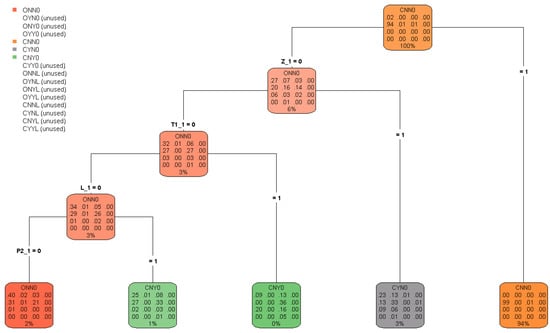
Figure 1. Frequency model: pruned classification tree for lag $\ell =1$.

The tree has $R_1=5$ leaves. In the “palette” associated with each node of the tree the corresponding frequency distribution of the response variable W observed in the calibration set ${\mathcal{D}}_1^C$ is reported. Therefore the palettes associated with the leaves provide the probability estimates ${\widehat{p}}_1^{(w,r)}$ associated with the regions ${\mathcal{R}}_1^{(r)},r=1,\dots ,5$, of the optimal partition ${\mathcal{P}}_1$, as shown by expression (15). Frequencies in the palettes are expressed in percent and are rounded to the nearest whole number. The rpart numerical output provides more precise figures.

To illustrate Figure 1 we order the leaves in sequence from left to right, so that the r-th leaf from the left corresponds to the region ${\mathcal{R}}_1^{(r)}$ of ${\mathcal{P}}_1$. Let us consider, for example, the claims in the fifth leaf ${\mathcal{R}}_1^{(5)}$, which have $\mathtt{Z}\_\mathtt{1}=1$. These are the claims in the calibration set that were closed at time 4 and 5 (then with $Z_{i,j|1-j}^{(\nu )}=1,i=3,4$); these claims are the $94\%$ of all claims in the calibration set. Since, under model assumptions, the observed frequencies provide the estimate of the corresponding probabilities at the current time I for event occurrences at time $I+1$, one can observe that for claims closed at time I there is (about) a $99\%$ probability that they will be closed without payments at time $I+1$, while there is (about) a $1\%$ probability that they will reopened with a payment. Leaf 4 in the tree contains the claims with $\mathtt{Z}\_\mathtt{1}=0$ and $\mathtt{T}\mathtt{1}\_\mathtt{1}=1$. These are the claims in the calibration set ($3\%$ of the total) which were open with a type-1 reserve placed on at time 4 and 5, i.e., $(Z_{i,j|1-j}^{(\nu )}=0)\cap ({\overline{R\mathit{1}}}_{i,j|1-j}^{(\nu )}=1),i=3,4$. From the frequency table reported in the palette, we conclude that for the claims open with type-1 reserve at time I the most probable state at time $I+1$ ($33\%$ probability) is CYN0, i.e., the state with a type-1 payment and claim closing ($W_{5,j|2-j}^{(\nu )}=5$). In leaf 3 we find the claims in the calibration set which at time 4 and 5 were open without type-1 reserve and with a lawyer involved, i.e., $(Z_{i,j|1-j}^{(\nu )}=0)\cap ({\overline{R\mathit{1}}}_{i,j|1-j}^{(\nu )}=0)\cap (L_{i,j|1-j}^{(\nu )}=1),i=3,4$. These claims are $0.2\%$ of the total. From the frequency table we conclude that for claims that at time I have the same feature the most probable state at time $I+1$ ($36\%$ probability) is CNY0, i.e., the state with a type-2 payment and claim closing ($W_{5,j|2-j}^{(\nu )}=6$). In the fourth binary split, which produces the first two leaves in the tree, the splitting criterion is the existence of a type-2 payment (indicator P2_1) for claims which at time 4 and 5 were open without type-1 reserve and without a lawyer. From the frequency tables in the second and the first leaf (referring to about $1\%$ and $2\%$ of the claims of the calibration set, respectively), one finds that if at time I the claim has a type-2 payment, the most probable state at time $I+1$ ($33\%$) is CNY0; otherwise the most probable state ($40\%$) is ONN0, i.e., it remains open without payments and without involving a lawyer.

It is interesting to note that although we included in the model also explanatory variables observed with historical depth $\theta =2$ (i.e., feature variables with subscript _0), none of these variables has been considered useful for prediction by the algorithm (after pruning). Only explanatory variables with $\theta =1$ (subscript _1) has been used for the splits in the pruned tree.

8.2. Possible Use for Early Warnings

For a given claim with $\ell =1$ let us consider questions as those of type (b) presented in Section 2 (with $\tau =1$). Formally, for a given claim ${\mathcal{C}}_{5,j}^{(\nu )}$ in ${\mathcal{D}}_1^P$ let us consider the event $\left\{{\mathcal{C}}_{5,j}^{(\nu )}will involve a lawyer at time 7\right\}$, with indicator $L_{5,j|2-j}^{(\nu )}$. This corresponds to the events $W_{5,j|2-j}^{(\nu )}\in \{8,\dots ,15\}$ hence:

$$\mathbb{P}\left[L_{5,j|2-j}^{(\nu )}=1\right]=\sum _{w=8}^{15}\mathbb{P}\left[W_{5,j|2-j}^{(\nu )}=w\right].$$

This probability is different in different leaves of the classification tree, then we write:

$${\lambda }^{(r)}:=\widehat{\mathbb{P}}\left[L_{5,j|2-j}^{(\nu )}=1|{\mathcal{C}}_{5,j}^{(\nu )}\in {\mathcal{R}}_1^{(r)}\right]=\sum _{w=8}^{15}{\widehat{p}}_1^{(w,r)},r=1,\dots R_1.$$

If $n^{(r)}$ denotes the number of claims ${\mathcal{C}}_{5,j}^{(\nu )}$ belonging to leaf r, the expected number of claims with lag 1 that will involve a lawyer in the next year is given by $\Lambda :={\sum }_{r=1}^{R_1}{\lambda }^{(r)}{n}^{(r)}$.

The values of ${\lambda }^{(r)}$ and $n^{(r)}$ are reported in Table 6, where the leaves are ordered by decreasing value of the probability ${\lambda }^{(r)}$. It results that the expected number is $\Lambda =920$. Since $|{\mathcal{D}}_1^P|={\sum }_{r=1}^5{n}^{(r)}=150,368$, only $0.6\%$ of the claims in ${\mathcal{D}}_1^P$ is expected to involve a lawyer in one year. This data could also be useful for providing information to an early-warning system. For example, a list could be provided of the first 323 claims in the table, i.e., the claims in ${\mathcal{D}}_1^P$ for which ${\lambda }^{(r)}>40\%$.

Table 6. Expectations of involving a lawyer in different leaves.

r	${\mathit{\lambda }}^{(\mathit{r})}$	${\mathit{n}}^{(\mathit{r})}$
3	40.50%	323
4	16.46%	3204
2	5.89%	1495
1	1.63%	1878
5	0.10%	143,468

In Section 11.2 we will present a backtesting exercise for this kind of predictions.

8.3. Prediction of Claim Payments Using the Conditional Severity Model

Once the optimal classification tree in Figure 1 has been obtained for the frequency, for each leaf in this tree two regression functions must be calibrated for the severity, one for type-1 and one for type-2 payments. For the sake of brevity, we illustrate two cases:

• The estimate of a type-1 (i.e., NoCARD) payment for open claims with type-1 reserve placed on, for which we consider the claims in leaf 4 in the frequency tree in Figure 1.
• The estimate of a type-2 (i.e., CARD) payment for open claims without type-1 reserve placed on and with lawyer involved, for which we consider the claims in leaf 3 in Figure 1.

Case 1. As pointed out in Section 7.3, since the severity model is a conditional model, for the calibration of the regression function ${\tilde{\mu }}_{\ell }^{(1)}$ only the claims for which a type-1 payment is made at the response date are considered. Hence the calibration set for this regression estimate is the subset of claims in leaf 4 of the frequency tree for which a type-1 payment was observed in the response. It results in this calibration set consisting of 2564 claims. For the calibration of this regression tree the following R command is used:

$$\begin{array}{cc}\hfill \mathtt{sevtree}\mathtt{4}<-\mathtt{rpart}(\mathtt{S}\mathtt{1}\_\mathtt{2}\sim & \mathtt{rd}+\mathtt{L}\_\mathtt{0}+\mathtt{L}\_\mathtt{1}+\mathtt{S}\mathtt{1}\_\mathtt{0}+\mathtt{S}\mathtt{1}\_\mathtt{1}+\mathtt{S}\mathtt{2}\_\mathtt{0}+\mathtt{S}\mathtt{2}\_\mathtt{1}+\hfill \\ \hfill & \mathtt{R}\mathtt{1}\_\mathtt{0}+\mathtt{R}\mathtt{1}\_\mathtt{1}+\mathtt{R}\mathtt{2}\_\mathtt{0}+\mathtt{R}\mathtt{2}\_\mathtt{1},\mathtt{data}=\mathtt{dt}\_\mathtt{sev}\mathtt{4},\hfill \\ \hfill & \mathtt{method}=‘\mathtt{anova}’,\mathtt{control}=\mathtt{rpart}.\mathtt{control}(\mathtt{cp}=\mathtt{0.001}))\hfill \end{array}$$

where dt_sev4 is the calibration set and the relabeling is used:

$$\begin{array}{cc}\hfill & {S\mathit{1}}_{i,j|2-j}^{(\nu )}=\mathtt{S}\mathtt{1}\_\mathtt{2},L_{i,j|1-j}^{(\nu )}=\mathtt{L}\_\mathtt{1},{S\mathit{1}}_{i,j|1-j}^{(\nu )}=\mathtt{S}\mathtt{1}\_\mathtt{1},{S\mathit{2}}_{i,j|1-j}^{(\nu )}=\mathtt{S}\mathtt{2}\_\mathtt{1},\hfill \\ \hfill & {R\mathit{1}}_{i,j|1-j}^{(\nu )}=\mathtt{R}\mathtt{1}\_\mathtt{1},{R\mathit{2}}_{i,j|1-j}^{(\nu )}=\mathtt{R}\mathtt{2}\_\mathtt{1},{\underline{j}}_i\le j\le 1;\hfill \\ \hfill & L_{i,0|0}^{(\nu )}=\mathtt{L}\_\mathtt{0},{S\mathit{1}}_{i,0|0}^{(\nu )}=\mathtt{S}\mathtt{1}\_\mathtt{0},{S\mathit{2}}_{i,0|0}^{(\nu )}=\mathtt{S}\mathtt{2}\_\mathtt{0},{R\mathit{1}}_{i,0|0}^{(\nu )}=\mathtt{R}\mathtt{1}\_\mathtt{0},{R\mathit{2}}_{i,0|0}^{(\nu )}=\mathtt{R}\mathtt{2}\_\mathtt{0}.\hfill \end{array}$$

As for the frequency case, after the large binary tree sevtree4 was grown by rpart, this was pruned using 10-fold cross-validation and applying the one-standard-error rule. The pruned tree thus obtained is illustrated in Figure 2, provided by rpart.plot.

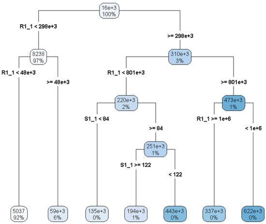
Figure 2. Severity model: pruned regression tree for claims in leaf 4 of the frequency tree.

The feature variable and its critical value used for the binary split are indicated on each node. On the palette attached to the node the empirical mean of payments and the percentage number of observations is reported. The partition provided by the pruned tree consists of 7 leaves. Under model assumptions, the average payment reported in the palette provides the expected value at time $I=6$ of the type-1 payment at time $I+1=7$.

Case 2. In this case, the calibration set for the severity tree is the subset of claims in leaf 3 of the frequency tree for which a type-2 payment was observed in the response. This calibration set consists of 281 claims. The R command used for this regression tree is similar to that for Case 1. The tree pruned with the usual method is reported in Figure 3.

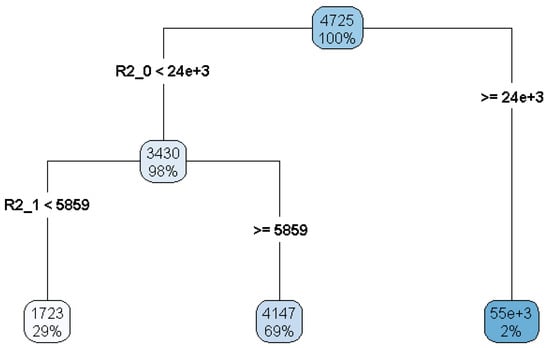
Figure 3. Severity model: pruned regression tree for claims in leaf 3 of the frequency tree.

The partition provided by this tree consists now of 3 leaves. The average payment reported in the palette of each leaf provides the expected value at time 6 of the type-2 payment at time 7 for these claims.

Part II. Multiperiod Predictions and Backtesting

9. Multiperiod Predictions

9.1. The Shift-Forward Procedure and the Self-Sustaining Property

The basic idea underlying the extension of a one-period prediction to a multiperiod prediction in the frequency model can be illustrated as follows. At time $i+j+k=I$, let us consider the claims referring to two contiguous prediction sets ${\mathcal{D}}_{\ell }^P,{\mathcal{D}}_{{\ell }^{\prime }}^P$ with ${\ell }^{\prime }=\ell +1,\ell =0,\dots ,I-3$, that is the claims classes:

$$\begin{array}{cc}\hfill \mathcal{H}& =\left({\mathcal{C}}_{i,j}^{(\nu )}:i=I-\ell ,{\underline{j}}_{I-\ell }\le j\le \ell ,1\le \nu \le N_{I-\ell ,j}\right),\hfill \\ \hfill {\mathcal{H}}^{\prime }& =\left({\mathcal{C}}_{i,j}^{({\nu }^{\prime })}:i=I-{\ell }^{\prime },{\underline{j}}_{I-{\ell }^{\prime }}\le j\le {\ell }^{\prime },1\le {\nu }^{\prime }\le N_{I-{\ell }^{\prime },j}\right).\hfill \end{array}$$

For these two classes the corresponding one-year prediction problem in the frequency model is given by:

$$\begin{array}{cc}\hfill \mathbb{E}\left[{\mathit{F}}_{I-\ell ,j|\ell -j+1}^{(\nu )}|{\mathcal{F}}_I\right]& =p_{\ell }^{(\mathit{f})}\left({\mathit{x}}_{I-\ell ,j|\ell -j}^{(\nu )}\right),\hfill \\ \hfill \mathbb{E}\left[{\mathit{F}}_{I-{\ell }^{\prime },j|{\ell }^{\prime }-j+1}^{({\nu }^{\prime })}|{\mathcal{F}}_I\right]& =p_{{\ell }^{\prime }}^{(\mathit{f})}\left({\mathit{x}}_{I-{\ell }^{\prime },j|{\ell }^{\prime }-j}^{({\nu }^{\prime })}\right).\hfill \end{array}$$

Assume that the prediction functions of the two problems have been calibrated on the sets ${\mathcal{D}}_{\ell }^C$ and ${\mathcal{D}}_{{\ell }^{\prime }}^C$ , respectively, with the resulting estimates for time $I+1$:

$$\begin{array}{ccc}\hfill {\widehat{\mathit{F}}}_{I-\ell ,j|\ell -j+1}^{(\nu )}& =& {\widehat{p}}_{\ell }^{(\mathit{f})}\left({\mathit{x}}_{I-\ell ,j|\ell -j}^{(\nu )}\right),\hfill \\ \hfill {\widehat{\mathit{F}}}_{I-{\ell }^{\prime },j|{\ell }^{\prime }-j+1}^{({\nu }^{\prime })}& =& {\widehat{p}}_{{\ell }^{\prime }}^{(\mathit{f})}\left({\mathit{x}}_{I-{\ell }^{\prime },j|{\ell }^{\prime }-j}^{({\nu }^{\prime })}\right).\hfill \end{array}$$

Our aim is to derive an estimate of the two-year response ${\mathit{F}}_{I-\ell ,j|\ell -j+2}^{(\nu )}$ for the claims ${\mathcal{C}}_{i,j}^{(\nu )}$ in class $\mathcal{H}$, i.e., with accident year $I-\ell$.

Assume that the feature and the response for claims in class $\mathcal{H}$ are specified so that:

$${\widehat{\mathit{F}}}_{I-\ell ,j|\ell -j+1}^{(\nu )}\supseteq {\widehat{\mathit{B}}}_{I-\ell ,j|\ell -j+1}^{(\nu )},$$

(17)

i.e., the estimated response variable for claims in class $\mathcal{H}$ contains an estimate of the next year dynamic component of the feature ${\mathit{x}}_{I-\ell ,j|\ell -j+1}^{(\nu )}$ of these claims, see expression (10). Following D’Agostino et al. (2018) a property such as (17) is referred to as self-sustaining property. Then we can estimate the response at time $I+2$ as:

$${\widehat{\mathit{F}}}_{I-\ell ,j|\ell -j+2}^{(\nu )}={\widehat{p}}_{\ell +1}^{(\mathit{f})}\left({\widehat{\mathit{x}}}_{I-\ell ,j|\ell -j+1}^{(\nu )}\right),$$

where ${\widehat{\mathit{x}}}_{i,j|I-i-j+1}^{(\nu )}={\left({\mathit{x}}_{i,j|I-i-j}^{(\nu )},{\widehat{\mathit{B}}}_{i,j|I-i-j+1}^{(\nu )}\right)}^{\prime }$ is the one-year updated feature of ${\mathcal{C}}_{i,j}^{(\nu )}\in \mathcal{H}$. In this procedure the two-year response estimate for claims in class $\mathcal{H}$ (whose one-year response has been estimated using the ${\widehat{\mu }}_{\ell }$ prediction function) is obtained by the ${\widehat{\mu }}_{{\ell }^{\prime }}$ prediction function, which has been estimated for claims in class ${\mathcal{H}}^{\prime }$ but is now applied to the claim feature updated using ${\widehat{\mu }}_{\ell }$.

The previous shift-forward procedure applied for all lags $\ell =0,\dots ,I-3$ provides all the two-year predictions, i.e., the entire “second new diagonal” of estimates in the “data triangle”, provided that property (17) holds for each lag.

As an example, let us consider in Table 7 the time I estimates for claims of accident year $I=6$ (class $\mathcal{H}$) and of accident year $I-1=5$ (class ${\mathcal{H}}^{\prime }$), with corresponding lags $\ell =0$ and ${\ell }^{\prime }=1$. We have the problems:

$$\mathbb{E}\left[{\mathit{F}}_{6,0|1}^{(\nu )}|{\mathcal{F}}_6\right]={\widehat{p}}_0^{(\mathit{f})}\left({\mathit{x}}_{6,0|0}^{(\nu )}\right),\mathbb{E}\left[{\mathit{F}}_{5,0/1|1/0+1}^{(\nu )}|{\mathcal{F}}_6\right]={\widehat{p}}_1^{(\mathit{f})}\left({\mathit{x}}_{5,0/1|1/0}^{(\nu )}\right),$$

which, after calibration at time 6 on ${\mathcal{D}}_0^C$ and ${\mathcal{D}}_1^C$, respectively, provide the estimates for time 7:

$${\widehat{\mathit{F}}}_{6,0|1}^{(\nu )}={\widehat{p}}_0^{(\mathit{f})}\left({\mathit{x}}_{6,0|0}^{(\nu )}\right),{\widehat{\mathit{F}}}_{5,0/1|1/0+1}^{(\nu )}={\widehat{p}}_1^{(\mathit{f})}\left({\mathit{x}}_{5,0/1|1/0}^{(\nu )}\right).$$

Table 7. Creating “future diagonals” by multiyear predictions.

We want to derive an estimate of the two-year response ${\mathit{F}}_{6,0|2}^{(\nu )}$ for the claims with accident year 6.

If ${\widehat{\mathit{F}}}_{6,0|1}^{(\nu )}\supseteq {\widehat{\mathit{B}}}_{6,0|1}^{(\nu )}$, i.e., if the one-year response variable for claims of accident year 6 includes an estimate of the next-year updating component of the features ${\mathit{x}}_{6,0|0}^{(\nu )}$, then we can estimate the response at time 8 as:

$${\widehat{\mathit{F}}}_{6,0|2}^{(\nu )}={\widehat{p}}_1^{(\mathit{f})}\left({\widehat{\mathit{x}}}_{6,0|1}^{(\nu )}\right),$$

where ${\widehat{\mathit{x}}}_{6,0|1}^{(\nu )}={\left({\mathit{x}}_{6,0|0}^{(\nu )},{\widehat{\mathit{B}}}_{6,0|1}^{(\nu )}\right)}^{\prime }$. This shift-forward procedure allowed by the self-sustaining property is represented in Table 7 by the first red arrow on the bottom. The same procedure applied for all lags $\ell =0,\dots ,I-3$ provides the entire “second new diagonal” of estimates i.e., the cells in light blue color in Table 7.

To derive the third new diagonal of estimates, i.e., the three-year predictions for lags $\ell =0,\dots ,I-3$, we can repeat the previous procedure, provided that the self-sustaining properties hold:

$${\widehat{\mathit{F}}}_{I-\ell ,j|\ell -j+2}^{(\nu )}\supseteq {\widehat{\mathit{B}}}_{I-\ell ,j|\ell -j+2}^{(\nu )},\ell =0,\dots ,I-3.$$

In the example of Table 7 the second shift-forward procedure providing the lowest element of the second new diagonal (darker blue cells) is represented by a blue arrow.

In general, for the h-th new diagonal, the required properties are:

$${\widehat{\mathit{F}}}_{I-\ell ,j|\ell -j+h}^{(\nu )}\supseteq {\widehat{\mathit{B}}}_{I-\ell ,j|\ell -j+h}^{(\nu )},h=1,\dots ,I-1,\ell =0,\dots ,I-1-h.$$

It should be noted that in all these multiyear prediction procedures only the calibrations for lags $\ell =0,\dots ,I-3$ made at time I are used.

9.2. Illustration in Terms of Partitions

The multiperiod prediction can be also illustrated in terms of partitions of $\mathcal{X}$. We refer here to the one-dimensional formulation of the frequency response. Following D’Agostino et al. (2018), in terms of the partition elements provided by the classification trees, the self-sustaining property requires that:

For $i=1,\dots ,I,j=0,\dots ,J,\nu =1,\dots ,N_{i,j},k\in {\mathbb{N}}_0$, the response $W_{i,j|k+1}^{(\nu )}$ and the features ${\mathit{x}}_{i,j|k}$, ${\mathit{x}}_{i,j|k+1}$ are such that for $u=1,\dots ,R_{j+k}$ and $w=0,1,\dots ,2^d-1$ it is always possible to calculate the function ${\varphi }_{j+k+1}(u,w)$ defined as:

$${\varphi }_{j+k+1}(u,w)=r:\left({\mathit{x}}_{i,j|k+1}^{(\nu )}\in {\mathcal{R}}_{j+k+1}^{(r)}\right)|\left(\left({\mathit{x}}_{i,j|k}^{(\nu )}\in {\mathcal{R}}_{j+k}^{(u)}\right)\cap \left(W_{i,j|k+1}^{(\nu )}=w\right)\right),r=1,\dots R_{j+k+1}.$$

That is for all $i,j,\nu ,k$ the features ${\mathit{x}}_{i,j|k}^{(\nu )},{\mathit{x}}_{i,j|k+1}^{(\nu )}$ and the response $W_{i,j|k+1}^{(\nu )}$ are specified so that any element of the partition ${\mathcal{P}}_{j+k}$ is mapped by ${\varphi }_{j+k+1}$ into a unique element of the partition ${\mathcal{P}}_{j+k+1}$. In principle, this could lead to formulate the multiyear prediction in terms of transition probabilities ${\pi }_{\ell }(u,w)$, i.e., the probability of transitioning from one state u of the response $W_{I-\ell ,j|\ell -j}^{(\nu )}$ to one state w of the response $W_{I-\ell ,j|\ell -j+1}^{(\nu )}$.

9.3. Illustration in Terms of Conditional Expectations

As in Wüthrich (2016) the multiperiod prediction can also be expressed in terms of conditional expectations. For the two-year prediction we have:

$$\begin{array}{cc}\hfill \mathbb{E}\left[{\mathit{F}}_{I-\ell ,j|\ell -j+2}^{(\nu )}|{\mathcal{F}}_I\right]& =\mathbb{E}\left[\mathbb{E}\left[{\mathit{F}}_{I-\ell ,j|\ell -j+2}^{(\nu )}|{\mathcal{F}}_{I+1}\right]|{\mathcal{F}}_I\right]\hfill \\ \hfill & =\mathbb{E}\left[\sum _{f_1,\dots ,f_d}{\mathit{f}}^{\prime }{p}_{\ell +1}^{(\mathit{f})}\left({\mathit{x}}_{I-\ell ,j|\ell -j+1}^{(\nu )}\right)|{\mathcal{F}}_I\right]\hfill \\ \hfill & =\sum _{f_1,\dots ,f_d}{\mathit{f}}^{\prime }\mathbb{E}\left[p_{\ell +1}^{(\mathit{f})}\left({\mathit{x}}_{I-\ell ,j|\ell -j+1}^{(\nu )}\right)|{\mathcal{F}}_I\right]\hfill \\ \hfill & =\sum _{f_1,\dots ,f_d}{\mathit{f}}^{\prime }{\widehat{p}}_{\ell +1}^{(\mathit{f})}\left({\widehat{\mathit{x}}}_{I-\ell ,j|\ell -j+1}^{(\nu )}\right),\hfill \end{array}$$

where in the last equality we replaced the probabilities $p_{\ell +1}^{(\mathit{f})}$ with their ${\mathcal{F}}_I$-measurable expectations provided by the CART calibration.

10. The Simulation Approach

The analytical calculations involved in both the transition matrix approach and the conditional expectation approach can be very burdensome from a computational point of view. The computational cost depends on the number of dynamic variables to be modeled. For example, with 4 dynamic variables and $I=10$ the number of possible states of the response W for a claim of accident year I is given by is $4^{2^{I-1}}=4^{2^9}=68,719,476,736$. To avoid these difficulties, we take a simulation approach for multiperiod forecasting.

10.1. A Typical Multiperiod Prediction Problem

To illustrate this approach, we consider one of the most important multiperiod prediction problems, which is the basis for individual claims reserving. In the outstanding portfolio, let us consider a specified claim ${\mathcal{C}}_{i,j}^{(\nu )}$ occurred in accident year i and reported with delay j. The claims portfolio has been observed up to the current date I and we want to predict on this date the total cost (of type 1 and type 2) in the next $\tau \in {\mathbb{N}}_1$ years. Let us define the cumulated costs:

$$\begin{array}{cc}\hfill & {K\mathit{1}}_{i,j|I-(i+j)+\tau }^{(\nu )}=\sum _{h=1}^{\tau }{S\mathit{1}}_{i,j|I-(i+j)+h}^{(\nu )},\tau \in {\mathbb{N}}_0,\hfill \\ \hfill & {K\mathit{2}}_{i,j|I-(i+j)+\tau }^{(\nu )}=\sum _{h=1}^{\tau }{S\mathit{2}}_{i,j|I-(i+j)+h}^{(\nu )},\tau \in {\mathbb{N}}_0,\hfill \end{array}$$

where, obviously, ${K\mathit{1}}_{i,j|I-(i+j)+0}^{(\nu )}={K\mathit{2}}_{i,j|I-(i+j)+0}^{(\nu )}=0$. We can say that ${({K\mathit{1}}_{i,j|I-(i+j)+\tau }^{(\nu )})}_{\tau \in {\mathbb{N}}_0}$ and ${({K\mathit{2}}_{i,j|I-(i+j)+\tau }^{(\nu )})}_{\tau \in {\mathbb{N}}_0}$ provide the cumulated cost development path, of type 1 and type 2 respectively, of the claim in the future, i.e., on the dates $I+1,I+2,\dots$. We want to predict these paths, i.e., we want to derive, using prediction trees, the estimates:

$$\begin{array}{cc}\hfill & {\widehat{K\mathit{1}}}_{i,j|I-(i+j)+\tau }^{(\nu )}=\widehat{\mathbb{E}}\left[{K\mathit{1}}_{i,j|I-(i+j)+\tau }^{(\nu )}|{\mathcal{F}}_I\right],\tau \in {\mathbb{N}}_1,\hfill \\ \hfill & {\widehat{K\mathit{2}}}_{i,j|I-(i+j)+\tau }^{(\nu )}=\widehat{\mathbb{E}}\left[{K\mathit{2}}_{i,j|I-(i+j)+\tau }^{(\nu )}|{\mathcal{F}}_I\right],\tau \in {\mathbb{N}}_1.\hfill \end{array}$$

In our data we have not observations to make predictions beyond the date $2I-1$, i.e., for $\tau >I-1$. If one assumes that the claims are finalized at this date, then we can take the expected cumulated cost at time $2I-1$ as an estimate of the individual reserve estimate, i.e.:

$$\begin{array}{cc}\hfill & {E\mathit{1}}_{i,j}^{(\nu )}={\widehat{K\mathit{1}}}_{i,j|2I-(i+j)-1}^{(\nu )}=\widehat{\mathbb{E}}\left[{K\mathit{1}}_{i,j|2I-(i+j)-1}^{(\nu )}|{\mathcal{F}}_I\right],\hfill \\ \hfill & {E\mathit{2}}_{i,j}^{(\nu )}={\widehat{K\mathit{2}}}_{i,j|2I-(i+j)-1}^{(\nu )}=\widehat{\mathbb{E}}\left[{K\mathit{2}}_{i,j|2I-(i+j)-1}^{(\nu )}|{\mathcal{F}}_I\right],\hfill \end{array}$$

(18)

where ${E\mathit{1}}_{i,j}^{(\nu )}$ and ${E\mathit{2}}_{i,j}^{(\nu )}$ denote the type-1 and type-2, respectively, reserve estimate at time I of the claim ${\mathcal{C}}_{i,j}^{(\nu )}$. The total reserve is obviously obtained as $E_{i,j}^{(\nu )}={E\mathit{1}}_{i,j}^{(\nu )}+{E\mathit{2}}_{i,j}^{(\nu )}$.

It is worth noting that if the case reserves are dynamically modeled, one could also obtain the estimates:

$$\begin{array}{cc}\hfill & {T\mathit{1}}_{i,j}^{(\nu )}:={\widehat{R\mathit{1}}}_{i,j|2I-(i+j)-1}^{(\nu )}=\widehat{\mathbb{E}}\left[{R\mathit{1}}_{i,j|2I-(i+j)-1}^{(\nu )}|{\mathcal{F}}_I\right],\hfill \\ \hfill & {T\mathit{2}}_{i,j}^{(\nu )}:={\widehat{R\mathit{2}}}_{i,j|2I-(i+j)-1}^{(\nu )}=\widehat{\mathbb{E}}\left[{R\mathit{2}}_{i,j|2I-(i+j)-1}^{(\nu )}|{\mathcal{F}}_I\right].\hfill \end{array}$$

(19)

If these estimates are different from zero the assumption of claims finalization at time $2I-1$ can be relaxed and the final case reserve estimates ${T\mathit{1}}_{i,j}^{(\nu )}$ and ${T\mathit{2}}_{i,j}^{(\nu )}$ can be used as type-1 and type-2, respectively, tail reserve estimates. In this case, one obtains comprehensive reserve estimates by adding the tail reserves in (19) to the estimates in (18).

10.2. Simulation of Sample Paths and Reserve Estimates

In the simulation approach the expected cumulated costs of the claim ${\mathcal{C}}_{i,j}^{(\nu )}$, and as a byproduct the reserve estimates, are obtained by simulating a number N of possible paths of the cost development and then computing the average path, which is obtained as the sample mean of the costs on each date of the paths. We give some details of this procedure. It is convenient to skip again to the “by lag” language in this exposition.

Let us suppose, as usual, that at time I the historical observations on the claims portfolio are sufficient for calibrating the classification tree for the frequency and the regression trees for the conditional severity (of type 1 and 2) for all lags $\ell =0,\dots ,I-2$. Therefore, at time I all the optimal frequency partitions ${\mathcal{P}}_{\ell }$ of the feature space $\mathcal{X}$ and the optimal severity partitions ${\mathcal{Q}}_{\ell }^{(1)},{\mathcal{Q}}_{\ell }^{(2)}$ corresponding to each leaf of ${\mathcal{P}}_{\ell }$ have been derived for $\ell =0,\dots ,I-2$.

Let ${\mathcal{C}}_{i,j}^{(\nu )}$ be a given claim in the portfolio, with at time I frequency feature ${\mathit{x}}_{i,j|\ell -j}^{(\nu )}$ and severity feature ${\tilde{\mathit{x}}}_{i,j|\ell -j}^{(\nu )}$, with $\ell =I-i$. The simulation procedure for the development cost of this claim is based on the following steps.

0.

Initialization. Set:

$${\ell }_0=\ell ,{K\mathit{2}}_{i,j|{\ell }_0-j}^{(\nu )}=0,{K\mathit{2}}_{i,j|{\ell }_0-j}^{(\nu )}=0,{\widehat{\mathit{x}}}_{i,j|{\ell }_0-j}^{(\nu )}={\mathit{x}}_{i,j|{\ell }_0-j}^{(\nu )},{\widehat{\tilde{\mathit{x}}}}_{i,j|{\ell }_0-j}^{(\nu )}={\tilde{\mathit{x}}}_{i,j|{\ell }_0-j}^{(\nu )}.$$

1.

Find the index r of the leaf of ${\mathcal{P}}_{{\ell }_0}$ to which the feature ${\widehat{\mathit{x}}}_{i,j|{\ell }_0-j}^{(\nu )}$ belongs.

2.

Simulate the state w of the frequency response ${\widehat{W}}_{i,j|{\ell }_0-j+1}^{(\nu )}$ at time ${\ell }_0+i+1$ using the probability distribution corresponding to the r-th leaf of ${\mathcal{P}}_{{\ell }_0}$.

3.

If w implies:

a.

a type-1 payment (i.e., a NoCARD payment) at time ${\ell }_0+i+1$, then assume as the expected paid amount at time ${\ell }_0+i+1$ the estimate ${\widehat{S\mathit{1}}}_{i,j|{\ell }_0-j+1}^{(\nu )}$ corresponding to the leaf of ${\mathcal{Q}}_{{\ell }_0}^{(1)}$ to which the feature ${\widehat{\tilde{\mathit{x}}}}_{i,j|{\ell }_0-j}^{(\nu )}$ belongs.

b.

a type-2 payment (i.e., a CARD payment) at time ${\ell }_0+i+1$, then assume as the expected paid amount at time ${\ell }_0+i+1$ the estimate ${\widehat{S\mathit{2}}}_{i,j|{\ell }_0-j+1}^{(\nu )}$ corresponding to the leaf of ${\mathcal{Q}}_{{\ell }_0}^{(2)}$ to which the feature ${\widehat{\tilde{\mathit{x}}}}_{i,j|{\ell }_0-j}^{(\nu )}$ belongs.

c.

no payments at time ${\ell }_0+i+1$, then all payments at time ${\ell }_0+i+1$ are set to 0.

4.

Set:

$${K\mathit{1}}_{i,j|{\ell }_0-j+1}^{(\nu )}={K\mathit{1}}_{i,j|{\ell }_0-j}^{(\nu )}+{\widehat{S\mathit{1}}}_{i,j|{\ell }_0-j+1}^{(\nu )},{K\mathit{2}}_{i,j|{\ell }_0-j+1}^{(\nu )}={K\mathit{2}}_{i,j|{\ell }_0-j}^{(\nu )}+{\widehat{S\mathit{2}}}_{i,j|{\ell }_0-j+1}^{(\nu )}.$$

5.

If ${\ell }_0<I-2$ then:

5.1.

The features ${\mathit{x}}_{i,j|{\ell }_0-j}^{(\nu )}$ and ${\tilde{\mathit{x}}}_{i,j|{\ell }_0-j}^{(\nu )}$ are updated with the new information provided by the responses ${\widehat{W}}_{i,j|{\ell }_0-j+1}^{(\nu )}$, ${\widehat{S\mathit{1}}}_{i,j|{\ell }_0-j+1}^{(\nu )}$ and ${\widehat{S\mathit{2}}}_{i,j|{\ell }_0-j+1}^{(\nu )}$, and the new features ${\widehat{\mathit{x}}}_{i,j|{\ell }_0-j+1}^{(\nu )}$ and ${\widehat{\tilde{\mathit{x}}}}_{i,j|{\ell }_0-j+1}^{(\nu )}$ are then obtained (this requires that the self-sustaining property holds).

5.2.

Set ${\ell }_0={\ell }_0+1$ and return to step 1.

With this procedure the two sample paths:

$${\left({K\mathit{1}}_{i,j|\ell -j+\tau }^{(\nu )}\right)}_{\tau =0,\dots ,I-1-\ell },{\left({K\mathit{2}}_{i,j|\ell -j+\tau }^{(\nu )}\right)}_{\tau =0,\dots ,I-1-\ell },$$

of the type-1 and type-2 cumulated cost are simulated for the chosen claim ${\mathcal{C}}_{i,j}^{(\nu )}$ with lag $\ell =I-i$. A simulation set of appropriate size is obtained with N independent iterations $h=1,\dots ,N$ of this procedure. The cost estimates are then obtained as the costs on the average path, i.e.,:

$$\begin{array}{cc}\hfill & {\widehat{K\mathit{1}}}_{i,j|\ell -j+\tau }^{(\nu )}=\frac{1}{N}\sum _{h=1}^N{}_h^{\phantom{|}}{K\mathit{1}}_{i,j|\ell -j+\tau }^{(\nu )},\hfill \\ \hfill & {\widehat{K\mathit{2}}}_{i,j|\ell -j+\tau }^{(\nu )}=\frac{1}{N}\sum _{h=1}^N{}_h^{\phantom{|}}{K\mathit{2}}_{i,j|\ell -j+\tau }^{(\nu )},\hfill \\ \hfill & \tau =0,\dots ,I-1-\ell .\hfill \end{array}$$

On the terminal date, i.e., for $\tau =I-1-\ell$, these sample averages provide the reserve estimates ${E\mathit{1}}_{i,j}^{(\nu )}$ and ${E\mathit{2}}_{i,j}^{(\nu )}$ in (18).

Once the CART approach has been extended to multiperiod predictions via simulation, it is convenient to make a further extension of the model to allow a joint dynamic modeling of the case reserves. Indeed, as anticipated in Section 5, to make the best use of the case reserve information in multiperiod predictions also the changes in the case reserve itself must be predicted by a specific model.

10.3. Including Dynamic Modeling of the Case Reserve

To dynamically model the case reserves, we extend the model assumptions in Section 4.2. Also, for the case reserve the conditional model is preferred, for the usual reason of a discrete probability mass typically present in 0 in the reserve distributions. Our additional assumptions are described as follows.

• The filtered probability space $(\mathsf{\Omega },\mathcal{F},\mathbb{P},\mathbb{F})$ must include also the two reserve processes:

  $${({R\mathit{1}}_{i,j|k}^{(\nu )})}_{i,j,k,\nu },{({R\mathit{2}}_{i,j|k}^{(\nu )})}_{i,j,k,\nu },$$

  which are $\mathbb{F}$-adapted for $t=i+j+k$ and for which the independency assumptions (H1), (H2), (H3) also hold.
• For the distribution of the case reserves a property similar to assumption (H5) holds, i.e.,:
  (HR5) For the conditional distribution of${R\mathit{1}}_{i,j|k}^{(\nu )}|({\overline{R\mathit{1}}}_{i,j|k}^{(\nu )}=1)$and${R\mathit{2}}_{i,j|k}^{(\nu )}|({\overline{R\mathit{2}}}_{i,j|k}^{(\nu )}=1)$one has:

  $$\begin{array}{cc}\hfill & {R\mathit{1}}_{i,j|k+1}^{(\nu )}|\left({\overline{R\mathit{1}}}_{i,j|k+1}^{(\nu )}=1\right)\sim \mathcal{N}\left({\dot{\mu }}_{j+k}^{(1)}\left({\dot{\mathit{x}}}_{i,j|k}^{(\nu )}\right),{\dot{\sigma }}_1^2\right),\hfill \\ \hfill & {R\mathit{2}}_{i,j|k+1}^{(\nu )}|\left({\overline{R\mathit{2}}}_{i,j|k+1}^{(\nu )}=1\right)\sim \mathcal{N}\left({\dot{\mu }}_{j+k}^{(2)}\left({\dot{\mathit{x}}}_{i,j|k}^{(\nu )}\right),{\dot{\sigma }}_2^2\right),\hfill \end{array}$$

  (20)

  where ${\dot{\mathit{x}}}_{i,j|k}^{(\nu )}\in \mathcal{X}$ is a ${\mathcal{F}}_{i+j+k}$-measurable feature of ${\mathcal{C}}_{i,j|k}^{(\nu )}$.
  As for the payment variables, these assumptions imply:

  $$\begin{array}{cc}\hfill & \mathbb{E}\left[{R\mathit{1}}_{i,j|k+1}^{(\nu )}|{\mathcal{F}}_{i+j+k},\left({\overline{R\mathit{1}}}_{i,j|k+1}^{(\nu )}=1\right)\right]={\dot{\mu }}_{j+k}^{(1)}\left({\dot{\mathit{x}}}_{i,j|k}^{(\nu )}\right),\hfill \\ \hfill & \mathbb{E}\left[{R\mathit{2}}_{i,j|k+1}^{(\nu )}|{\mathcal{F}}_{i+j+k},\left({\overline{R\mathit{2}}}_{i,j|k+1}^{(\nu )}=1\right)\right]={\dot{\mu }}_{j+k}^{(2)}\left({\dot{\mathit{x}}}_{i,j|k}^{(\nu )}\right),\hfill \end{array}$$

  where the conditional expectations can be calibrated by regression trees. Then there exists an ${\mathcal{F}}_{i+j+k}$-measurable severity feature ${\tilde{\mathit{x}}}_{i,j|k}^{(\nu )}$ which determines the conditional expectation of the cash flows ${S\mathit{1}}_{i,j|k}^{(\nu )}$ and ${S\mathit{2}}_{i,j|k}^{(\nu )}$. The unconditional reserve expectations are then given by:

  $$\begin{array}{cc}\hfill & \mathbb{E}\left[{R\mathit{1}}_{i,j|k+1}^{(\nu )}|{\mathcal{F}}_{i+j+k}\right]={\dot{\mu }}_{j+k}^{(1)}\left({\dot{\mathit{x}}}_{i,j|k}^{(\nu )}\right)\mathbb{P}\left[{\overline{R\mathit{1}}}_{i,j|k+1}^{(\nu )}=1|{\mathcal{F}}_{i+j+k}\right],\hfill \\ \hfill & \mathbb{E}\left[{R\mathit{2}}_{i,j|k+1}^{(\nu )}|{\mathcal{F}}_{i+j+k}\right]={\dot{\mu }}_{j+k}^{(2)}\left({\dot{\mathit{x}}}_{i,j|k}^{(\nu )}\right)\mathbb{P}\left[{\overline{R\mathit{2}}}_{i,j|k+1}^{(\nu )}=1|{\mathcal{F}}_{i+j+k}\right].\hfill \end{array}$$
• To further improve the predictive performance, an assumption similar to assumption (H4) or (H4’) can be added, which we express here in the one-dimensional form (8):
  (HR4’) For the conditional distribution of:

  $${\dot{W}}_{i,j|k}^{(\nu )}={\overline{R\mathit{1}}}_{i,j|k}^{(\nu )}+2{\overline{R\mathit{2}}}_{i,j|k}^{(\nu )},$$
  one has:

  $${\dot{W}}_{i,j|k+1}^{(\nu )}=w|{\mathcal{F}}_{i+j+k},\left(Z_{i,j|k+1}^{(\nu )}=0\right)\sim \mathrm{Categorical}\left({\dot{p}}_{j+k}^{(w)}\left({\mathit{x}}_{i,j|k}^{(\nu )}\right)\right),$$

  (21)

  where ${\dot{p}}_{j+k}^{(w)}:\mathcal{X}\mapsto {[0,1]}^4$ is a probability function, i.e.:

  $$\sum _{w=0}^3{\dot{p}}_{j+k}^{(w)}\left({\mathit{x}}_{i,j|k}^{(\nu )}\right)=1.$$
  This assumption implies:

  $$\mathbb{P}\left[{\dot{W}}_{i,j|k+1}^{(\nu )}=w|{\mathcal{F}}_{i+j+k},\left(Z_{i,j|k+1}^{(\nu )}=0\right)\right]={\dot{p}}_{j+k}^{(w)}\left({\mathit{x}}_{i,j|k}^{(\nu )}\right)\ge 0,w=0,\dots ,3.$$

Assumption (HR4’) is not required if there is only one type of payment, since if we have, say, only type-1 payments, then ${\overline{R\mathit{1}}}_{i,j|k+1}^{(\nu )}=1-Z_{i,j|k+1}^{(\nu )}$.

We can consider additional conditioning in expression (20) and/or (21) in order to better modeling particular effects. For example, one could condition on the state of the indicator $Z_{i,j|k}^{(\nu )}$ at the previous date in order to distinguish predictions concerning open claims and reopened claims. All these enhancements of the model have been applied in the following examples.

10.4. Example of Simulated Cost Development Paths

Using the simulation procedure illustrated in Section 10.2 and the additional assumptions presented in the previous section we can provide examples of multiperiod predictions including the joint dynamic modeling of case reserves. We provide here an example of cost development path simulation for an individual claim, using the data on the same claims portfolio of examples in Section 8. Before considering a specific claim, we derived all the frequency and the severity partitions for all lags $\ell =0,\dots ,4$ by calibrating prediction trees on the entire claims portfolio. The run time of all these calibrations is roughly 3 min on a workstation with one 8-core Intel processor@3.60 GHz (4.30 GHz max turbo) and 32 GB RAM. We then considered an individual claim with the following characteristics:

·

accident year: $i=I=6$;

·

reporting delay: $j=0$, hence we denote the claim as ${\mathcal{C}}_{6,0}^{(\nu )}$;

·

the claim is open at time I: $Z_{6,0|0}^{(\nu )}=0$;

·

the claim does not involve a lawyer at time I: $L_{6,0|0}^{(\nu )}=0$;

·

no type-1 (NoCARD) payment made at time I: ${\overline{S\mathit{1}}}_{6,0|0}^{(\nu )}=0$;

·

no type-2 (CARD) payment made at time I: ${\overline{S\mathit{2}}}_{6,0|0}^{(\nu )}=0$;

·

type-1 reserve at time I: ${R\mathit{1}}_{6,0|0}^{(\nu )}=31,460$ euros;

·

type-2 reserve at time I: ${R\mathit{2}}_{6,0|0}^{(\nu )}=13,820$ euros.

Since $i=I$ we start with ${\ell }_0=0$ in the simulation procedure, which provides the maximum length sample paths $\left({K\mathit{1}}_{6,0|0}^{(\nu )},{K\mathit{1}}_{6,0|1}^{(\nu )},\dots ,{K\mathit{1}}_{6,0|5}^{(\nu )}\right)$ and $\left({K\mathit{2}}_{6,0|0}^{(\nu )},{K\mathit{2}}_{6,0|1}^{(\nu )},\dots ,{K\mathit{2}}_{6,0|5}^{(\nu )}\right)$. In each simulation an execution of the predict.rpart function was invoked for each lag. The computation time required for simulating all sample paths (for the type-1 and type-2 cost) is roughly 4 min. In Figure 4 and Figure 5 $N=5000$ simulated sample paths for the type-1 and type-2 cumulated cost, respectively, of ${\mathcal{C}}_{6,0}^{(\nu )}$ are reported. Since many paths overlap, the simulated paths are shown in blue with the color depth being proportional to the number of overlaps. The average paths in the two figures are shown in red: their final point corresponds to ${\widehat{K\mathit{1}}}_{6,0|5}^{(\nu )}=17,069$ euros and ${\widehat{K\mathit{2}}}_{6,0|5}^{(\nu )}=4314$ euros. If we assume that the claims are finalized at time 11, i.e., after $\tau =5$ years for this claim, then these amounts can be taken as an estimate of the individual claim reserves ${E\mathit{1}}_{6,0}^{(\nu )}$ and ${E\mathit{2}}_{6,0}^{(\nu )}$ to be placed at the current date on ${\mathcal{C}}_{6,0}^{(\nu )}$. This suggests significant decreases in both the outstanding case reserves, namely a decrease of $14,391$ euros for ${R\mathit{1}}_{6,0|0}^{(\nu )}$ and a decrease of 7406 euros for ${R\mathit{2}}_{6,0|0}^{(\nu )}$.

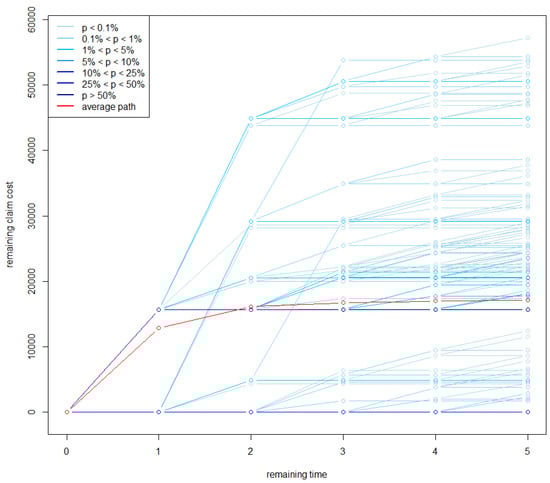
Figure 4. Representation of $N=5000$ simulated paths for the type-1 cost development of the chosen claim ${\mathcal{C}}_{6,0}^{(\nu )}$. In red the average path is reported.

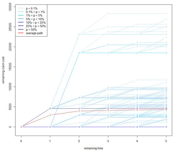
Figure 5. Representation of $N=5000$ simulated paths for the type-2 cost development of the chosen claim ${\mathcal{C}}_{6,0}^{(\nu )}$. The average path is in red.

It is interesting to note that with this dynamic approach we also have an estimate of the tail reserves ${T\mathit{1}}_{6,0}^{(\nu )}$ and ${T\mathit{2}}_{6,0}^{(\nu )}$ which are obtained as the average of the 5000 simulated values of ${\widehat{R\mathit{1}}}_{6,0|5}^{(\nu )}$ and ${\widehat{R\mathit{2}}}_{6,0|5}^{(\nu )}$. These estimates result in being ${T\mathit{1}}_{6,0}^{(\nu )}=386$ euros and ${T\mathit{2}}_{6,0}^{(\nu )}=248$ euros, which should be added to the corresponding expected cumulated costs, thus giving ${E\mathit{1}}_{6,0}^{(\nu )}=17,455$ euros and ${E\mathit{2}}_{6,0}^{(\nu )}=4562$ euros.

The variation coefficient in the simulated sample is $63.6\%$ for type-1 reserve and $91.6\%$ for type-2 reserve. The relative standard error of the mean is $0.9\%$ and $1.3\%$, respectively.

Whether the reserve adjustments indicated by the model are actually done could depend on a specific decision. However, these findings should suggest putting the claim under scrutiny.

11. Testing Predictive Performance of CART Approach

In this section, we propose some backtesting exercises in order to get some insight into the predictive performance of our CART approach. We first illustrate backtesting results for predictions of one-year event occurrences useful for claim watching. Multiperiod occurrence predictions could be similarly tested. Finally, we perform a typical claim reserving exercise, which is composed of two steps. In a first step the individual reserve estimate is derived by simulation for all the claims in the portfolio and the resulting total reserve (after the addition of an IBNYR reserve estimate) is compared with the classical chain-ladder reserve, which is estimated on aggregate payments at portfolio level. We perform these estimates on data deprived of the last calendar year observations. Then in a second step we can assess the predictive performance of the CART approach with respect to the chain-ladder approach by comparing the realized aggregate payments in the “first next diagonal” with those predicted by the two methods.

11.1. The Data

In these predictive efficiency tests, we need to calibrate the CART models assuming time $I-1$ as the current date, since observations at time I are used to measure the forecast error. For this reason, data on claims portfolio used in the previous section has not sufficient historical depth. We then use in this section a different dataset containing a smaller variety of claim features (in particular, the variables $L_{i,j|k}^{(\nu )}$ are not present) but a longer observed claims history. We have:

·

Observed accident years: from 2007 to 2016. Then $i=1,\dots ,10$.

·

All claims reported are observed, hence for accident year i one has $j=0,\dots ,10-i$ (i.e., ${\underline{j}}_i\equiv 0$).

Then there are 55 blocks $(i,j)$ in the original dataset. The total number of reported claims is 1,337,329. However, since we use claims observed in year 2016 (i.e., responses with $i+j+k=10$) for testing predictions, we assume $I=9$ as the current date and we drop from the original dataset all claims with $i+j=10$ and all observations with $i+j+k=10$. This reduces the data for the calibration to 9 observed accident years (45 $(i,j)$ blocks). In this data the pairs feature-response are observed for lags $\ell =0,\dots ,I-3=7$. The total number of reported claims in this portfolio observed at time $I=9$ is ${\sum }_{i,j}{N}_{i,j}=1,211,392$. The number of observations in the calibration set and the prediction set of each lag is reported in Table 8.

Table 8. Number of observations in the calibration and the prediction set of each lag in the claims portfolio observed at time $I=9$.

ℓ	$|{\mathcal{D}}_{\mathit{\ell }}^{\mathit{C}}|$	$|{\mathcal{D}}_{\mathit{\ell }}^{\mathit{P}}|$
0	1,012,099	121,633
1	964,302	119,075
2	852,271	116,207
3	732,116	121,885
4	592,538	139,828
5	445,686	146,965
6	296,880	148,895
7	144,310	152,593

11.2. Prediction of One-Year Event Occurrences

We test the predictive efficiency of some one-year event predictions considering the indicators of type-1 payment, type-2 payment and closure for lag $\ell =0$, i.e., we consider the predicted responses ${\widehat{Z}}_{9,0|1}^{(\nu )},{\widehat{\overline{S\mathit{1}}}}_{9,0|1}^{(\nu )},{\widehat{\overline{S\mathit{2}}}}_{9,0|1}^{(\nu )}$ for $\nu =1,\dots ,N_{9,0}$, i.e., for all the $|{\mathcal{D}}_0^P|=N_{9,0}=121,633$ claims in block $(9,0)$. These response estimates were provided by the classification tree for the frequency calibrated on ${\mathcal{D}}_0^C$ ($1,012,099$ observations). Since these responses are actually observed at time 10, we can assess the predictive performance of the model by comparing predicted and realized values. To this aim, we refer to a specific forecasting exercise.

For a given indicator, let us denote as positive, or negative, a claim in the sample ${\mathcal{D}}_0^P$ for which the indicator will be 1, or 0, respectively. Our forecasting exercise consists of predicting not only how many claims in the sample will be positive, but also which of them will be positive. i.e., we want to provide the claim code cc of the $\Lambda$ claims in the sample we predict as positive, where $\Lambda$ is the number of claims we expect to be positive. Our prediction strategy is very intuitive. Let ${\mathcal{R}}_0^{(r)},r=1,\dots ,R_0$, the r-th leaf of the partition ${\mathcal{P}}_0$ provided by the calibrated frequency tree. Using notations introduced in Section 8.2, we denote by $n^{(r)}$ the number of claims belonging to ${\mathcal{R}}_0^{(r)}$ and by ${\lambda }^{(r)}$ the probability to be positive for each of these claims. We assume that the leaves are ordered by decreasing value of ${\lambda }^{(r)}$ and define $r^{*}=min\{r:N^{(r)}\le \Lambda \}$, where $N^{(r)}={\sum }_{h=1}^r{n}^{(h)}$. Our forecasting strategy consists then in predicting as positive all the $N^{(r^{*})}$ claims in the first $r^{*}$ leaves and, in addition, $\Lambda -N^{(r^{*})}$ claims which are randomly chosen among those in leaf $r^{*}+1$.

The accuracy of our prediction could be measured by introducing an appropriate gain/loss function giving a specified (positive) score to claims correctly classified and a specified (negative) score to claims incorrectly classified. The choice of such a function, however, depends on the specific use one makes of the prediction, then in order to illustrate the results we prefer to resort here to the so-called confusion matrices, which we present in Figure 6. In these matrices blue (brown) cells refer to predicted (realized) values, green (red) cells refer to claims correctly (incorrectly) classified.

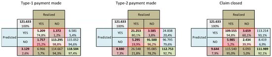
Figure 6. Confusion matrices for prediction of payment and closure indicators for claims with $\ell =0$.

Let us consider, for example, the first matrix, concerning the indicator ${\widehat{\overline{S\mathit{1}}}}_{9,0|1}^{(\nu )}$, i.e., {A type-1 payment is made in the next year}. We observe that 6581 claims of the $121,633$ in the prediction set, i.e., the $5.4\%$, were predicted by the model to have a type-1 payment, while type-1 payments actually realized were 6966 ($5.7\%$). Of the 6581 claims predicted as positive, 5209 resulted in being true positive (TP, green cell) and the remaining 1372 were false positive (FP, red cell). Considering the $115,052$ claims predicted to have not a type-1 payment, i.e., to be negative, 1757 resulted in being false negative (FN, red cell) and the remaining $113,295$ were true negative (TN, green cell). Then, globally, $118,504$ claims were correctly predicted ($97.4\%$ of all the predicted claims) and the remaining 6966 were incorrectly predicted. Ratios typically used are also reported, as:

·

True positive ratio, also known as sensitivity: TPR = TP/(TP+FN)$=74.8\%$;

·

True negative ratio, or specificity: TNR = TN/(TN+FP)$=98.8\%$;

·

False negative ratio: FNR $=1-$ TPR$=25.2\%$;

·

False positive ratio: FPR $=1-$ TNR$=1.2\%$.

The other two matrices have the same structure.

11.3. Prediction of Aggregate Claims Costs

11.3.1. Aggregate RBNS Reserve as Sum of Individual Reserves

We performed the CART calibration for the frequency-severity model extended with the dynamic case reserve model for all the 8 lags in the time-9 dataset. Given the large number of claims in this portfolio these calibrations required 73 min for computations. After the model calibration, for each of the 1,211,392 claims reported at time 9 we simulated $N=50$ cost development paths for the type-1 and type-2 payments using the procedure illustrated in Section 10 and we computed the corresponding average paths. In each simulation and for each lag the predict.rpart function can be invoked only one time for all claims with the same lag. With respect to the simulation of a single claim, this provides, proportionally, a substantial reduction of computation time. The run time for all the simulations was roughly 120 min.

By computing the incremental payments of each average path and summing over the entire portfolio we obtained a CART reserve estimate for the reported but not settled (RBNS) claims. If these total payments are organized by accident year (on the rows) and payment date (on the column) we obtain a “lower triangle” of estimated future payments with the same structure of the usual lower triangles in classical claims reserving.

By the simulation procedure the individual reserve estimates are provided:

$$\begin{array}{cc}\hfill & {\widehat{K\mathit{1}}}_{i,j|8-j}^{(\nu )}=\frac{1}{N}\sum _{h=1}^N{}_h^{\phantom{|}}{K\mathit{1}}_{i,j|8-j}^{(\nu )},\hfill \\ \hfill & {\widehat{K\mathit{2}}}_{i,j|8-j}^{(\nu )}=\frac{1}{N}\sum _{h=1}^N{}_h^{\phantom{|}}{K\mathit{2}}_{i,j|8-j}^{(\nu )},\hfill \\ \hfill & {\widehat{K}}_{i,j|8-j}^{(\nu )}={\widehat{K\mathit{1}}}_{i,j|8-j}^{(\nu )}+{\widehat{K\mathit{2}}}_{i,j|8-j}^{(\nu )},\hfill \\ \hfill & i=2,\dots ,9,j=0,\dots 9-i,\nu =1,\dots ,N_{i,j}.\hfill \end{array}$$

Assuming claims finalization at time $2I-1=17$, one obtains from these cost estimates the corresponding RBNS reserves, at different levels of aggregation:

$$\begin{array}{cc}\hfill & {E\mathit{1}}_i^{R\mathit{B}NS}:=\sum _{j=0}^{9-i}\sum _{\nu =1}^{N_{i,j}}{\widehat{K\mathit{1}}}_{i,j|8-j}^{(\nu )},i=2,\dots ,I;{E\mathit{1}}^{R\mathit{B}NS}=\sum _{i=2}^9{E\mathit{1}}_i^{R\mathit{B}NS};\hfill \\ \hfill & {E\mathit{2}}_i^{R\mathit{B}NS}:=\sum _{j=0}^{9-i}\sum _{\nu =1}^{N_{i,j}}{\widehat{K\mathit{2}}}_{i,j|8-j}^{(\nu )},i=2,\dots ,I;{E\mathit{2}}^{R\mathit{B}NS}=\sum _{i=2}^9{E\mathit{2}}_i^{R\mathit{B}NS};\hfill \\ \hfill & E^{R\mathit{B}NS}={E\mathit{1}}^{R\mathit{B}NS}+{E\mathit{1}}^{R\mathit{B}NS}.\hfill \\ \hfill \end{array}$$

(22)

The simulation procedure also provides the individual tail reserve estimates:

$$\begin{array}{cc}\hfill & {\widehat{R\mathit{1}}}_{i,j|8-j}^{(\nu )}=\frac{1}{N}\sum _{h=1}^N{}_h^{\phantom{|}}{\widehat{R\mathit{1}}}_{i,j|8-j}^{(\nu )},\hfill \\ \hfill & {\widehat{R\mathit{2}}}_{i,j|8-j}^{(\nu )}=\frac{1}{N}\sum _{h=1}^N{}_h^{\phantom{|}}{\widehat{R\mathit{2}}}_{i,j|8-j}^{(\nu )},\hfill \\ \hfill & {\widehat{R}}_{i,j|8-j}^{(\nu )}={\widehat{R\mathit{1}}}_{i,j|8-j}^{(\nu )}+{\widehat{R\mathit{2}}}_{i,j|8-j}^{(\nu )},\hfill \\ \hfill & i=1,\dots ,9,j=0,\dots 9-i,\nu =1,\dots ,N_{i,j},\hfill \end{array}$$

which can be aggregated as:

$$\begin{array}{cc}\hfill & {T\mathit{1}}_i=\sum _{j=0}^{9-i}\sum _{\nu =1}^{N_{i,j}}{\widehat{R\mathit{1}}}_{i,j|8-j}^{(\nu )},i=1,\dots ,I;T\mathit{1}=\sum _{i=1}^9{T\mathit{1}}_i;\hfill \\ \hfill & {T\mathit{2}}_i=\sum _{j=0}^{9-i}\sum _{\nu =1}^{N_{i,j}}{\widehat{R\mathit{2}}}_{i,j|8-j}^{(\nu )},i=1,\dots ,I;T\mathit{2}=\sum _{i=1}^9{T\mathit{2}}_i;\hfill \\ \hfill & T=T\mathit{1}+T\mathit{2}.\hfill \end{array}$$

These estimates can be added to the corresponding estimates in (22) in order to provide an adjustment of the reserves computed under the assumption of finalization at time $2I-1$.

As usual, the aggregate claim cost estimates can be organized by accident year and by development year (dy), indexed as $h=0,\dots ,I-1$, where in the CART model “development year” is a new wording for the “lag” $I+\tau -i$. With this representation we obtain the “lower triangle” for the total costs (type 1 + type 2) reported in Table 9 in green color.

Table 9. Aggregate lower triangle of the incremental RBNS cost estimates and corresponding RBNS reserves. In the last two rows the adjustments for IBNYR claims are reported.

ayi	$\mathtt{dy}=1$	$\mathtt{dy}=2$	$\mathtt{dy}=3$	$\mathtt{dy}=4$	$\mathtt{dy}=5$	$\mathtt{dy}=6$	$\mathtt{dy}=7$	$\mathtt{dy}=8$	reserve: ${\mathit{E}}_{\mathit{i}}^{\mathbf{RBNS}}$	CoVa${}_{\mathit{i}}$
1	$·$	$·$	$·$	$·$	$·$	$·$	$·$	$·$	0	$0.00\%$
2	$·$	$·$	$·$	$·$	$·$	$·$	$·$	548,939	548,939	$5.51\%$
3	$·$	$·$	$·$	$·$	$·$	$·$	841,939	660,135	1,502,074	$9.12\%$
4	$·$	$·$	$·$	$·$	$·$	1,336,090	989,338	679,961	3,005,388	$5.50\%$
5	$·$	$·$	$·$	$·$	1,989,568	1,352,147	1,026,083	663,033	5,030,831	$6.18\%$
6	$·$	$·$	$·$	2,652,175	1,842,702	1,266,884	799,521	595,623	7,156,905	$3.63\%$
7	$·$	$·$	4,658,838	2,609,709	1,584,964	1,170,623	725,353	569,174	11,318,662	$2.97\%$
8	$·$	10,672,731	4,061,362	2,479,849	1,849,869	1,104,580	693,130	543,766	21,405,288	$1.66\%$
9	32,184,296	7,479,426	3,467,081	2,644,659	1,819,141	1,158,269	685,487	593,554	50,031,913	$1.11\%$
RBNS diagonal	54,884,575	18,994,820	10,504,823	7,127,705	4,244,697	2,420,573	1,229,253	593,554	100,000,000	$\mathbf{0}.\mathbf{79}\%$
IBNYR	5,393,583	1,416,003	688,614	518,063	341,608	220,980	126,677	95,314	8,800,841
RBNS+IBNYR	60,278,158	20,410,822	11,193,436	7,645,768	4,586,305	2,641,554	1,355,930	688,868	108,800,841

Figures in the aggregate “upper triangle” (pink color) are not reported in order to point out that this kind of data were not used for the prediction. Total estimated costs summed by diagonal (highlighted by different green intensity) as well as summed by accident year (second last column) are also reported. For confidentiality reasons all paid amounts in this numerical example were rescaled so as to obtain a total reserve $E^{R\mathit{B}NS}=100,000,000$ euros. For each accident year reserve estimate and for the total estimate the coefficient of variation on the simulated sample was computed. These figures, reported in the last column of the table, are rather low. This should be explained by the fact that each aggregate reserve simulation is the sum of a very large number of individual claim costs and the correlation among these individual costs is very low. Obviously, this weak correlation is also a consequence of the independence assumptions in the model.

11.3.2. Inclusion of the IBNYR Reserve Estimate

We are interested in comparing the CART reserve estimates with the classical chain-ladder reserve estimates. To allow this comparison a cost estimate for IBNYR claims must be added to the aggregate RBNS reserve derived in the previous section. Therefore, we complemented the RBNS reserve model with an ancillary model for the IBNYR reserve, which is outlined in Appendix A. This model is a “severity extension” of the “frequency approach” proposed in Wüthrich (2016) for estimating the expected number of IBNYR claims. The results of the ancillary model estimates are summarized (after rescaling) in the second last row of Table 9, where the IBNYR reserves, by diagonal and overall, are reported. Figures in the last row provide the corresponding RBNS claim reserves adjusted for IBNYR claims.

Remark 5.

This separation between RBNS and IBNYR claims is in some respect similar to that obtained in Verral et al. (2010).

11.3.3. Comparison with Chain-Ladder Estimates

In the chain-ladder approach to classical claims reserving the sums of all the individual claim payments in the portfolio observed up to time I are organized by accident year and development year and an upper triangle of observed paid losses, cumulated along development in each accident year, is obtained. The reserve estimates are then derived by the cumulated paid losses in the lower triangle, which is obtained by applying to the upper triangle the well-known chain-ladder algorithm. This is shown in Table 10 where, to allow comparison with Table 9, incremental payments are reported.

Table 10. Chain-ladder reserve estimates on aggregate payments (type-1+type-2, incremental figures). The differences with the CARTs estimates are also reported.

ayi	$\mathtt{dy}=0$	$\mathtt{dy}=1$	$\mathtt{dy}=2$	$\mathtt{dy}=3$	$\mathtt{dy}=4$	$\mathtt{dy}=5$	$\mathtt{dy}=6$	$\mathtt{dy}=7$	$\mathtt{dy}=8$	Reserve ${\mathit{E}}_{\mathit{i}}^{\mathbf{CL}}$
1	35,699,311	37,879,857	12,003,345	6,478,312	3,033,793	1,895,577	1,026,086	922,252	497,792	0
2	41,730,803	36,146,954	14,363,454	4,928,858	3,051,338	2,913,180	1,237,083	899,977	529,656	529,656
3	40,033,745	31,396,571	13,499,535	5,668,671	2,719,742	2,314,666	856,136	868,753	489,839	1,358,592
4	39,027,439	38,571,568	12,499,545	6,084,483	2,903,344	2,930,986	1,075,959	928,216	523,367	2,527,541
5	39,143,444	37,227,132	11,612,033	4,676,458	2,897,767	2,477,989	1,033,956	891,980	502,936	4,906,860
6	33,900,305	33,987,815	11,872,716	5,088,186	2,644,290	2,268,885	946,706	816,711	460,496	7,137,087
7	31,820,892	33,590,427	10,841,703	4,822,608	2,526,694	2,167,983	904,604	780,390	440,016	11,642,296
8	33,667,137	32,084,528	11,173,371	4,865,109	2,548,961	2,187,090	912,576	787,268	443,894	22,918,269
9	39,151,374	37,275,145	12,987,380	5,654,965	2,962,788	2,542,166	1,060,734	915,081	515,961	63,914,221
CL diagonal	$·$	60,867,772	25,100,078	12,733,962	7,374,128	4,695,628	2,288,018	1,358,976	515,961	114,934,523
CL—CARTs	$·$	589,614	4,689,256	1,540,526	−271,640	109,323	−353,535	3,046	−172,907	6,133,683
%	$·$	1.0%	23.0%	13.8%	−3.6%	2.4%	−13.4%	0.2%	−25.1%	5.6%

As in Table 9 the upper triangle is highlighted in pink and the lower triangle in green, and the chain-ladder reserves at different aggregation levels—by diagonal, by accident year, overall—are computed. In the last two rows of the table the differences with the CART estimates in the last row of Table 9 are shown. In some diagonals, i.e., in some future calendar years, there are substantial differences between the chain-ladder and the CART claims cost predictions. However, the overall chain-ladder reserve estimate is $5.6\%$ higher than the corresponding CART estimate. When the results provided by the two methods are compared, one should take into account that the chain-ladder estimates do include an underwriting year inflation forecast, since an estimate of historical underwriting year inflation is implicitly projected on future dates by the algorithm. In the CART approach, instead, some degree of expected inflation might be implicitly included in the predicted costs only through the case reserves. An additional component of expected inflation must however be added to the reserve estimates. A similar problem is found in DCL model, see Martínez-Miranda et al. (2013) for an estimation method of the underwriting year inflation based on incurred data.

11.3.4. Backtesting the Two Methods on the Next Diagonal

Since we deliberately made the reserve estimates for a claims portfolio observed at time 10 (i.e., 2016) using only data observed up to time 9 (2015), we are now able to perform a backtest on the “first next diagonal” since next-year realized payments (of both type 1 and type 2) are actually known. In Table 11 the realized payments and the prediction errors (i.e., realized − predicted) of the two methods are reported for accident years $2\le i\le 9$.

Table 11. Forecast errors of CARTs and chain-ladder method on the next-year claim payments.

ay: i	Realized	Chain-ladder	(%)	CART	(%)
	Payments	Error		Error
2 (2008)	586,099	$-56,443$	$-9.63$	$-37,109$	$-6.33$
3 (2009)	1,145,117	$-276,364$	$-24.13$	$-284,528$	$-24.85$
4 (2010)	2,272,564	$-1,196,605$	$-52.65$	$-916,852$	$-40.34$
5 (2011)	1,734,932	$743,057$	$42.83$	$279,561$	$16.11$
6 (2012)	3,129,167	$-484,877$	$-15.50$	$-445,027$	$-14.22$
7 (2013)	3,902,228	$920,380$	$23.59$	$872,408$	$22.36$
8 (2014)	10,637,406	$535,965$	$5.04$	$394,152$	$3.71$
9 (2015)	38,117,533	$-842,388$	$-2.21$	$-1,109,494$	$-2.91$
total	61,525,046	$-\mathbf{657},\mathbf{275}$	$-\mathbf{1}.\mathbf{07}$	$-\mathbf{1},\mathbf{246},\mathbf{889}$	$-\mathbf{2}.\mathbf{03}$

The backtest exercise shows important errors in some accident years for both the methods. The overall predictions, however, are rather good for the two methods, showing an under-estimate of $1.07\%$ by chain-ladder and $2.03\%$ by CARTs. Considering possible adjustments for the expected inflation of CART prediction, we can say that in this case the predictive accuracy of the two methods is roughly similar.

Remark 6.

In this backtesting exercise the chain-ladder method has good predictive performance on the total reserve and is not easy to improve. A better assessment of the predictive efficiency of the CART approach in providing estimates of the aggregate reserve as sum of individual reserves could be obtained in cases where the chain-ladder approach poorly performs. For example, repeating the same exercise on different claims data (which for the moment are not authorized for disclosure), we observed on the total reserve estimate a forecast error of $18.64\%$ with the chain-ladder and $-5.10\%$ with the CART approach.

12. Conclusions

The CART approach illustrated in this paper seems promising for claims reserving and, more generally, for the claim watching activity. The large model flexibility of CARTs allows inclusion in the model of effects in the claims development process, which are difficult to study with classical methods. CARTs are rather efficient also in variable selection. However, the role of expert opinions in the choice of the explanatory variables to be included in the model is still important. Also, in this respect the interpretability of the results provided by CARTs can be very helpful.

Prediction and claims handling methods provided by the CART approach can also have an impact on business organization, in so far as they suggest and promote a closer connection into the insurance firm between the actuarial and the claims settlement activity.

As usual, the reliability of the results depends crucially on the quality of data available. In the proposed CART applications, it is also true, however, that enlarging the richness of data can also extend the scope and the significance of the results. For example, if information at individual policy level is included in the dataset, our CART approach could also provide indications useful for non-life-insurance pricing.

As is well known, a main disadvantage of CARTs is that they are not very robust towards changes in the data, since a small change in the observations may lead to a largely different optimal tree. Also, the sensitivity of the optimal tree to changes of the calibration parameters should be carefully analyzed. Random forests are proposed as the natural answer to the instability problem; however, the interpretability of the results is an important property which should not be lost. Backtesting exercises as those presented in this paper could help to get the instability effects under control.

References

- Breiman, Leo, Jerome H. Friedman, Richard A. Olshen, and Charles J. Stone. 1998. Classification and Regression Trees. London: Chapman & Hall/CRC. [Google Scholar]
- D’Agostino, Luca, Massimo De Felice, Gaia Montanucci, Franco Moriconi, and Matteo Salciarini. 2018. Machine learning per la riserva sinistri individuale. Un’applicazione R.C. Auto degli alberi di classificazione e regressione. Alef Technical Reports No. 18/02. Available online: http://alef.it/doc/TechRep_18_02.pdf (accessed on 9 October 2019).
- Gabrielli, Andrea, Richman Ronald, and Mario V. Wüthrich. 2018. Neural network embedding of the over-dispersed Poisson reserving model. Scandinavian Actuaria Journal, 1–29. [Google Scholar] [CrossRef]
- Hastie, Trevor, Robert Tibshirani, and Jerome Friedman. 2008. The Elements of Statistical Learning. Data Mining, Inference, and Predictions, 2nd ed. Springer Series in Statistics; Berlin: Springer. [Google Scholar]
- Hiabu, Munir, Carolin Margraf, Maria Dolores Martínez-Miranda, and Jens Perch Nielsen. 2015. The link between classical reserving and granular reserving through double chain ladder and its extensions. British Actuarial Journal 21: 97–116. [Google Scholar] [CrossRef]
- Martinez-Miranda, Maria Dolores, Bent Nielsen, Jens Perch Nielsen, and Richard Verrall. 2011. Cash Flow Simulation for a Model of Outstanding Liabilities Based on Claim Amounts and Claim Numbers. Astin Bulletin 41: 107–29. [Google Scholar]
- Martínez-Miranda, Maria Dolores, Jens Perch Nielsen, and Richard Verrall. 2012. Double Chain Ladder. ASTIN Bulletin 42: 59–76. [Google Scholar]
- Martínez-Miranda, Maria Dolores, Jens Perch Nielsen, and Richard Verrall. 2013. Double Chain Ladder and Bornhuetter-Ferguson. North American Actuarial Journal 17: 101–13. [Google Scholar] [CrossRef][Green Version]
- Pešta, Michal, and Ostap Okhrin. 2014. Conditional least squares and copulae in claims reserving for a single line of business. Insurance: Mathematics and Economics 56: 28–37. [Google Scholar] [CrossRef]
- Taylor, Greg. 2019. Claim Models: Granular and Machine Learning Forms. Sydney: School of Risk and Actuarial Studies, University of South Wales. [Google Scholar]
- Taylor, Greg, Gráinne McGuire, and James Sullivan. 2008. Individual claim loss reserving conditioned by case estimates. Annals of Actuarial Science 3: 215–56. [Google Scholar] [CrossRef]
- Therneau, Terry M., Elizabeth J. Atkinson, and Mayo Foundation. 2015. An Introduction to Recursive Partitioning Using the RPART Routines. R Vignettes, version of June 29. Rochester: Mayo Foundation. [Google Scholar]
- Verrall, Richard, Jens Perch Nielsen, and Anders Hedegaard Jessen. 2010. Prediction of RBNS and IBNR claims using claim amounts and claim counts. ASTIN Bulletin 40: 871–87. [Google Scholar]
- Verrall, Richard J., and Mario V. Wüthrich. 2016. Understanding reporting delay in general insurance. Risks 4: 25. [Google Scholar] [CrossRef]
- Wüthrich, Mario V. 2016. Machine Learning in Individual Claims Reserving. Research Paper No. 16-67. Zürich: Swiss Finance Institute. [Google Scholar]
- Wüthrich, Mario V., and Christoph Buser. 2019. Data Analytics for Non-Life Insurance Pricing. Research Paper No. 16-68. Zürich: Swiss Finance Institute. Available online: https://ssrn.com/abstract=2870308 (accessed on 9 October 2019).
- Wüthrich, Mario V., and Michael Merz. 2019. Editorial: Yes, we CANN! ASTIN Bulletin 49: 1–3. [Google Scholar] [CrossRef]