Abstract
It is intuitive that proximity to hospitals can only improve the chances of survival from a range of medical conditions. This study examines the empirical evidence for this assertion, based on Australian data. While hospital proximity might serve as a proxy for other factors, such as indigenity, income, wealth or geography, the evidence suggests that proximity provides the most direct link to these factors. In addition, as it turns out, a very statistically significant one that transcends economies.
JEL Classification:
I1; I11; R11
1. Introduction
The case of Australia provides an appropriate setting for a proximity study as it is very diverse in terms of hospital locations and population densities, not unlike the United States or Canada, but less densely populated than most parts of Europe or Asia. Whilst there are some studies of the effect of hospital proximity on the outcome of particular conditions (for example, the effect of hospital proximity on young road traffic victims in the UK Bentham (1986)), Nicholl discusses the effect of proximity based on ambulance data, and claims that age, sex and illness are not significant factors. However, that study was for the UK, where distances are much smaller than in Australia. Nonetheless, this paper is broadly consistent with those quantitative findings, allowing for the greater distances involved and the emergency of the situation.
Infant mortality Karra et al. (2017) has also been studied across a range of countries, which are also broadly in line with this paper. This study thus provides a quantitative first step with the general conclusion that proximity affects an increase in mortality according to region; it may provide insight into the optimum location of hospitals, and perhaps the facilities that should be provided to deal with certain conditions.
The geographic and spatial dimensions of mortality have long been recognized, particularly with respect to particular conditions such as cancer and heart disease Haining (2017). There are many variables that affect regional mortality, such as ethnicity, income, familiarity as well as local amenity. In such studies, the issue of heteroscedasticity in statistical models is particularly serious Fung et al. (2017), especially when historical analysis and forecasting are involved.
This paper adopts a simple approach by avoiding all the factors that might be incidentally associated with region. It is based on an Australian census, conducted every three years. Whilst regional data are provided as part of the survey, the only relevance to this paper is the proximity to hospitals that the population enjoys (or suffers), and not any other incidental factor that location might provide. It is possible that proximity is a proxy for income and wealth variables—which are either unavailable or inaccessible. Thus, we are not focused on mortality trends; indeed, the results of this paper highlight the pitfalls of doing so.
In summary, this paper is broadly consistent with the proximity studies cited above, given their limited scope. First, it is relevant to the planning and location of hospitals. Second, it throws a different light on insurance pricing and design.
2. Data
Data were provided by the Australian Bureau of Statistics (ABS) from the inter-census period 2005–2007 Australian Bureau of Statistics (2010), which was used to construct the Australian Life Tables relating to that period. Population data related to the mid-census year 2006 and mortality data to the inter-census period; these were reasonably consistent with the data published in the Australian Life Tables 2005–07 (ALT) Australian Government Actuary (2009). It is acknowledged that more recent data are available, but, given the difficulty in acquiring that data, this should not detract from the principles involved in this study. It should be noted that mortality relates to a three-year period, so that the mortality rates in this study need to be divided by 3 to provide annualized rates.
The statistics were subdivided by age, sex and statistical division (SD). The SD is a concept used by the ABS to denote geographical location: there are 61 SDs in total, covering all states, territories and dependencies in Australia. In this paper, the terms SD and ‘region’ are used interchangeably. The origin of SDs is purely historical and political, based on the establishment of the various Australian states and their settlement since colonization. Thus, they do not afford a truly objective basis for studying mortality, a theme to which we return in this paper.
Of the 61 SDs, mortality data were provided for only 59 SDs. No data were provided for ‘Other Territories’, which cover the outlying islands. Canberra and the Australian Capital Territory were amalgamated into a single SD for the purpose of this study as no separate data was provided for the latter.
The SDs are defined by the ABS in terms of geographical polygons, giving the longitude and latitude of their vertices. This information is available in ESRI shapefile format, which facilitates the calculation of distances and the plotting of charts, as is set out below1. In this study, all positions, distances and areas are expressed in terms of degrees of latitude and longitude, with 1 in spherical coordinates being approximately 60 nautical miles.
Though age was a relevant factor, mortality statistics were provided only to the age of 85. All statistics after that age were aggregated at age 85. The reason is that deaths after that age in individual SDs are few in number and would be identifiable, so it appears that privacy considerations prevail.
The ABS also provided population data for 1755 cities and towns across Australia in the mid census year (the smallest town having a population of only 24), together with their geographical coordinates. Again, this should not detract from the principles involved in this study.
Hospital data were provided by the Australian Institute of Health and Welfare Australian Institute of Health and Welfare (2017), an agency of the Australian government. Hospitals were categorized by the number of beds and geographical location. For the purpose of this study, only 347 of these hospitals, both private and public, have been included, as the number of 50 beds is considered to be the minimum for providing emergency care in critical conditions (such as accidents, cardiac arrest and stroke).
A depiction of the various town/city locations, and those of hospitals, is set out below in Figure 1.
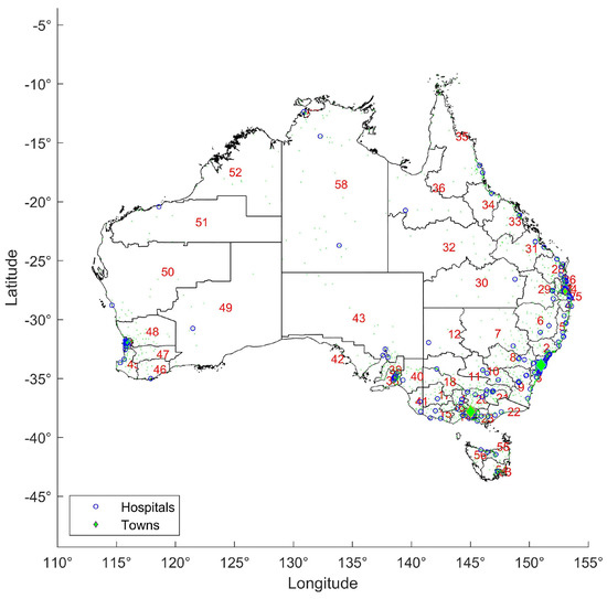
Figure 1.
Towns and hospitals.
2.1. Notation
Denote:
- x age next birthday, for ,
- r region, for ,
- city within region r,
- h hospital,
- age dependent mortality for age x,
- number of deaths at age x in region r,
- number of exposed lives at age x in region r,
- population of city contained in region r,
- the distance (in degrees) from to the nearest hospital
Since not all the population in a given SD resides in a city or town, we assume that the rural population is distributed uniformly within the region and assess the average nearest distance to a hospital accordingly. The technicalities are set out in Appendix A.
Overall statistics in terms of geography, population, urbanization and hospitalization are set out in the following table. The towns in the ‘Other Territories’ are excluded from Table 1 below.

Table 1.
Regional statistics.
It is evident that some SDs are poorly serviced by hospitals—for example, the Northern Territory and Kimberley SDs. These may coincide with the areas of the highest indigenous population. We do not speculate on the reasons for this, whether it be the economics of low population density or the outcome of government health policy. However, a rural population is included with the assessment of the each SD, giving a notional rural population in and its associated hospital proximity .
2.2. A General Model
We hypothesize that deaths D can be explained by natural mortality and the town/city populations within each region, along with the distances of those cities from hospitals. Thus, we investigate a model of the form
where
- is the strength of age-based hospital proximity effects;
- the population-weighted distance to the nearest hospital;
- is a variance term (see below);
- is a normal error term with constant variance.
In general, the suffixes r and x are omitted where the meaning is clear from context.
The variance in the above model allows for heteroscedasticity. It is well known that both the Poisson and binomial models may be approximated by a normal distribution, where the population is high in relation to the mortality rate. This is a result of the Central Limit Theorem. Thus, a ‘continuous’ Poisson distribution may be adopted Ilienko (2013).2
Under the Poisson model for mortality, we could take or under the binomial Alternatively, we could regard the proximity effect as part of the overall mortality, and take In general, we avoid the binomial model in favor of the Poisson, which is simpler and leads to much of the same results. Under a negative binomial approach, for some constant . All of these approaches, which are of increasing complexity, are examined below, in order to assess whether the errors may be found to be normal and have constant (hopefully unit) variance.
As with most statistical mortality models Venter (2001), the method of estimating the parameters in the model is taken as that of maximum likelihood (ML). In this instance, the likelihood is
and thus the log likelihood is, up to an additive constant3,
An appropriate formula for model comparison is the Akaike Information Criterion Brockett (1991)4 that allows for the number of parameters (whether in or ) to be estimated, and favours models with the lowest level of
3. The Model with Heteroscedasticity
Though it is possible to examine models with homoscedastic errors, i.e., is constant across ages and regions, we do not do so as the assumption is entirely unrealistic, as it would not take account of population size. Thus, some form of heteroscedasticity needs to be assumed. It is instructive to consider models with and without proximity effects, in order to gauge their overall significance. The truism is that neglecting heteroscedasticity produces unbiased but inefficient estimators. Thus, mortality estimates may suffer unwarranted volatility.
3.1. The Model without Proximity or Regionality
The raw ALT rates may be derived rigorously by considering a model of the form
where with being a constant across all and ages and regions. The estimators for this model are the naive ratios that ignore regional data completely
However, the estimates of the variance parameter are less intuitive
and with
This type of model has several shortcomings. First, the variance term , whilst allowing the greatest errors for the greatest populations, does not allow for ages where mortality is lowest (say near birth) or highest. Second, it does not discriminate between regions of different age structure and/or mortality. The statistics are poor, which is not surprising as the model does not give any credence to regional data.
3.2. The Model with Regionality but Not Proximity
It is clear that the general model above encapsulates the case where proximity effects are absent, i.e., This may provide a first approximation to the parameter q in the general model. It is of interest in its own right, as it allows comparison with the graduated rates set out in ALT.
In this case, we take , and the estimators for q from maximizing the log likelihood can be derived analytically:
where is the number of SDs. This is a result of the more general model in Section 4, where and
A comparison of these estimated mortality rates, which allow for heteroscedasticity, and both the raw and graduated rates set out in ALT2005-07 are in Figure 2 as follows.
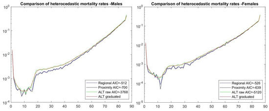
Figure 2.
Regional mortality rates.
It is apparent that, by allowing for heteroscedasticity, which favors the regions with the lowest mortality rates, and thus volatility of deaths, the estimated rates are generally lower than those derived in ALT without such considerations, and with lower inter-age volatility. The graduated rates Australian Government Actuary (2009) were reached using cubic splines and human judgement, so it is not possible to ascribe an However they would not differ significantly from that for the raw rates.
A Regionalized Model
Another model assumes that age and regional effects can be separated:
again with and with overall mortality This is referred to as a ‘Regionalized Model’. It has a high and is the nearest competitor to models with proximity, as it allows for regional effects to manifest directly. This may be depicted in Figure 3 below.
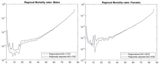
Figure 3.
Regionalized mortality rates = by age.
Under this regionalized model, it is possible to identify the SDs with the highest overall mortality, being those with the highest This is depicted graphically in Figure 4 as follows.
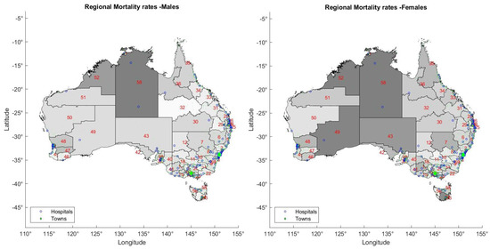
Figure 4.
Regionalized mortality rates—by region.
It comes as no surprise that the SDs with the highest mortality are also those with the highest level of indigenity and sparsest population. It also appears that females do not receive the same level of medical care as males in male dominated regions, where mining or farming predominate. However, it would be highly ethically challenging to price insurance on such as a basis, as this would be arbitrary and discontinuous (for example, how would borderline populations be treated?). To this end, we examine the relevance of an objective variable, which is continuous and largely determined by the population itself, namely proximity to hospitals and medical care. This is the antithesis to regionality.
4. The Model with Proximity
Where proximity effects are allowed for, it is not always possible to derive analytic expressions. Thus, numerical optimization is needed. However the result is that mortality rates specific to both age and proximity may be estimated. To test the robustness of the model from a statistical viewpoint, we employ the to assess whether proximity effects are justified.
The simplest form of a proximity model may be written
where Note that, in this version, the regional factors in Section 3.2 (which are applied to ) are replaced by age-based proximity factors (which are applied to the regional distance data in ). Fortunately, the ML estimates of the parameters and in this simplest version of the model extend the regional model in Section 2, and may be found in closed form. The details are set out in Appendix B.
The significance of the proximity factors may be assessed from the and bounds for the factors in Figure 5:
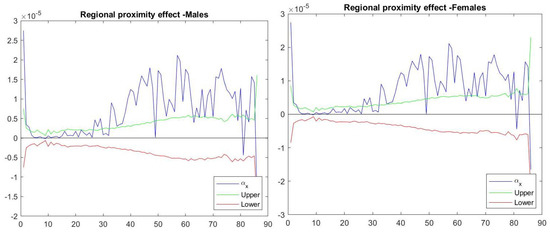
Figure 5.
Bounds for regional mortality factors.
The charts suggest the significance of the proximity factors at the 95% level. However, this type of proximity model has to be diagnosed for the structure of its residual errors, and how they compare with regionally based models. This is the subject of the next section.
5. Diagnostics
It remains to assess whether the residuals arising from estimation of the various models satisfy the usual assumptions of normality.
There are two possible explanations for any absence of normality. The first is that the residuals do not in fact obey a Poisson distribution, which assumes independence of deaths. This is highly likely in an industrial context. The second explanation is simply that the recording of deaths is subject to error, either in terms of age or location of death. Thus, the diagnostics of the residual errors are undertaken with and without exclusion of ages/regions where the number of deaths is recorded as being 6 or below (i.e., less than two deaths per annum). Some 47% of regional/age groups fall into this category,
Since the negative binomial distribution (NB) allows for over dispersion of residuals, we examine whether it provides a better fit to the data. In biostatistics, the Negative Binomial allows for contagion in deaths Kemp and Kemp (2005) and has been successfully employed for mortality data. The Poisson model gives both the mean and variance of deaths as . In contrast, by assuming nonindependence of deaths, the NB gives a variance of for some contagion parameter c. Thus, the variance cannot be directly proportional to exposures. We may extend this to the case where the underlying mortality is affected by proximity. i.e., with
The mortality estimates under both the Poisson and Negative Binomial (NB) models are as follows in Figure 6:
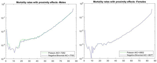
Figure 6.
Comparative mortality rates.
To assess the residuals, normal probability plots are given for the errors as shown below. The following chart examines the residuals resulting from the Poisson model in Figure 7.
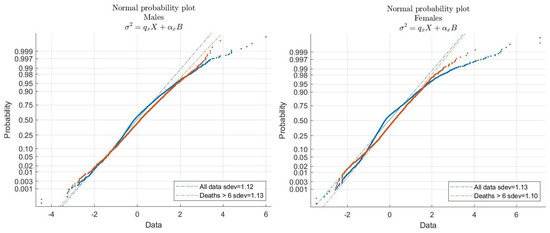
Figure 7.
Normal probability plot—Poisson.
The following chart examines the residuals resulting from the Negative Binomial model in Figure 8.
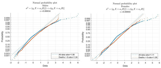
Figure 8.
Normal probability plot—negative binomial.
It may be observed that the residual errors, with the variances shown, do (almost) satisfy the assumption of constant (unit) variance. However, the plots are left (i.e., negatively) skewed.
The conclusion is that the effect of allowing for non-Poisson residuals has only a slight effect on the estimation of the mortality rates and proximity effects. However, they do resolve the issues of skewness and normality with the Poisson model, as the standard deviations of the NB residuals are close to unity, the presumption in estimation.
Moreover, the contagion parameters c in the NB model have a real significance: that for males is well above that for females . The obvious explanation is that males are engaged en masse to a greater extent than females in hazardous industries, such as in mining, energy and construction.
The strength of the proximity effect is tabulated in Appendix C, being the ratio of the proximity effect to total mortality rate The overall effect is small, being dominated by the capital cities, but very significant for some regions. It is not surprising that sparsely populated regions suffer most from the tyranny of distance, notably in the Kimberley and Pilbara, which are mining regions. The major cities are much better served for medical treatment and enjoy the least tyranny of distance. However, there are a few, perhaps counterintuitive, observations.
Expressed as a percentage of total mortality, the proximity effect per 10 km is set out in Appendix D (using 1 nautical mile = 1.852 km). These results indicate overall that 10 km distance is consistent with no more than a 1% increase in mortality rate, a result consistent with the UK Nicholl et al. (2007) but applied to much larger distances in Australia and to all conditions, even those not involving ambulances.
Proximity effects appear strongest near birth, or during the teenage years. This would attest to the efficacy of medical treatment for these age groups, which suffer from accidental causes that are most effectively treated when administered in a timely manner. Infant mortality is also significant and with distances of 10 km are consistent with a 27% increase in mortality Karra et al. (2017).
A surprising result is that proximity for the elderly is a negative factor, even strongly negative in sparse regions, for year 85 onwards. This does not suggest that the elderly suffer from being close to medical treatment. Rather, it suggests that those with terminal illnesses gravitate to where such treatment is more readily available, and vice versa.
A summary of the various models above is as follows in Table 2:
Table 2.
Comparison of .
6. Indigenity
It is controversial why the indigenous people—the aborigines—suggest higher mortality rates than others. The impact on national mortality is limited—they comprise just 3.3% of the population5.
The greatest population is in the Northern Territory (SD 58) and Western Australia (SDs 49–52). While 80% and 40%, respectively, live in remote regions of these SDs, 80% of the total population lives in urbanized areas overall. There are two competing theories for the higher indigenous mortality in regions where they predominate:
- their lifestyle and culture leads to riskier outcomes (a racist argument); or
- their remoteness from health care.
The proximity effects of Appendix D (proximity effect per 10 km) suggest the latter, as it is a form of deprivation. However, much greater data are needed to confirm this conclusion.
7. Conclusions
From a comparison of homoscedastic and heteroscedastic models for mortality, it becomes glaringly obvious that the variance of mortality rates is essential to their estimation. It is also evident that age is not the only explanatory factor in modelling mortality. Region, but more tellingly hospital proximity, is a vital factor. Proximity is a continuous and objective rating factor, largely chosen by the individual that can be employed on a logical and defensible basis. For this to be undertaken appropriately, the structure of residual errors must be chosen carefully. The results of this paper, and common logic, suggest the Negative Binomial for modelling contagion in populations.
The other observation that can be made is that there are numerous difficulties (indeed futility), with forecasting mortality. It is a truism that medical advances drive the trends in mortality, as do warfare and technology. This paper illustrates that the accessibility to medical treatment is equally important.
Unfortunately, this has political and financial dimensions. It is intuitive that distance affects mortality in a causal fashion, as the time taken to be hospitalized impacts directly the promptness of treatment, which is critical for many conditions, especially for the young, and, for example, cardiac conditions and stroke. This aspect is presumed in all the literature Nicholl. The issue then becomes the costs of establishing a hospital, with the appropriate medical facilities, in a given location versus the benefits to the local community. This is beyond the scope of this paper.
Funding
This research received no external funding.
Conflicts of Interest
The author declares no conflict of interest.
Appendix A. Assessing the Impact of Rural Areas
The bulk of the population in each SD is in the cities and towns, for which precise geographical coordinates are known, and the distance from the nearest hospital calculated. However, a significant proportion lies in rural areas, especially for the less developed SDs. For want of better information, we assume that rural populations are distributed uniformly within each SD.
To calculate the average nearest distance for these rural populations is no trivial matter, as the SDs themselves, which are defined by polygons, are in some cases non-convex, or even not simply connected (as there are a large number of islands on Australia’s coastline). Though straightforward in principle, the following procedure may be adopted:
- The ‘catchment area’ of each hospital is calculated. This is a polygon whose interior consists of points, all of which have the given hospital as its nearest. The polygon may be constructed by drawing a line segment between a given hospital, and all other hospitals, and then taking a perpendicular through the midpoint of each line segment, The perpendiculars establish the catchment area of each hospital. By definition, the catchment areas cannot intersect. The process is illustrated in Figure A1 below for SD = 58, which includes numerous outlying islands.
- Each SD is divided into catchment areas for the various hospitals. It should be noted that a hospital need not actually be in a SD, as some remote regions have their nearest hospital in another SD.
- The intersection of SDs and catchment areas is polygons which themselves may not be simply connected. Thus, for the purpose of assessing average nearest distance, a triangulation of each polygon must be made. Integration over the triangles comprising each polygon may then be undertaken to calculate average nearest distance. The results for each SD are set out in Table 1.
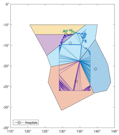
Figure A1.
Northern Territory Triangulation by hospital catchment area.
Appendix B. The Model with Proximity
We examine the heteroscedastic model
with log likelihood
Dropping subscripts, the first derivatives of are
and
For simplicity of notation, denote . Then, the above derivatives may be written as
and
From these first derivatives, we may calculate the second derivatives. It is clear that the off diagonal terms in , and are zero. Hence, the only non-zero terms are:
Equating the first derivatives to zero for a minimum in we get and substituting in Label (A1)
which simplifies to
and hence an exact ML estimator for q is:
We take the positive root above since and from Cauchy’s inequality. In the case that we have and the expression for reduces to that in Equation (1).
The Hessian matrix, which is used to assess the variance of the estimators, is then given by evaluating the second derivatives at the value for
For convenience of notation, note that refers to the diagonal matrix with as its diagonal, etc.
Since can be partitioned into four diagonal matrices, its inverse can be determined exactly:
where The Fisher information matrix may then be used to assess error bounds for the parameter estimates in Section 4.
Appendix C
Table A1.
Proximity Effects—Males.
Table A1.
Proximity Effects—Males.
| SD | Statistical Division | 1–5 | 6–10 | 11–15 | 16–20 | 21–25 | 26–30 | 31–35 | 36–40 | 41–45 | 46–50 | 51–55 | 56–60 | 61–65 | 66–70 | 71–75 | 76–80 | 81–85 | ≥ 86 | Total |
|---|---|---|---|---|---|---|---|---|---|---|---|---|---|---|---|---|---|---|---|---|
| 1 | Sydney | 1.9% | 1.1% | 0.8% | 5.4% | 3.6% | 2.2% | 1.9% | 2.6% | 2.4% | 1.5% | 0.7% | 0.8% | 0.6% | 0.5% | 0.3% | 0.2% | 0.1% | 0.0% | 0.5% |
| 2 | Hunter | 13.4% | 7.7% | 5.5% | 28.9% | 23.9% | 18.2% | 15.1% | 18.5% | 16.2% | 9.7% | 4.8% | 4.8% | 3.5% | 3.1% | 1.9% | 1.1% | 0.6% | −0.1% | 2.7% |
| 3 | Illawarra | 6.1% | 3.1% | 2.2% | 13.9% | 11.4% | 8.5% | 6.8% | 8.6% | 7.0% | 4.1% | 2.0% | 2.0% | 1.4% | 1.1% | 0.7% | 0.4% | 0.2% | −0.1% | 1.1% |
| 4 | Richmond-Tweed | 6.2% | 3.1% | 2.1% | 13.4% | 13.3% | 10.0% | 7.6% | 8.7% | 6.9% | 3.6% | 1.7% | 1.7% | 1.4% | 1.1% | 0.6% | 0.3% | 0.2% | 0.0% | 0.9% |
| 5 | Mid-North-Coast | 17.9% | 9.3% | 6.2% | 34.7% | 37.2% | 29.4% | 22.9% | 25.3% | 20.2% | 11.5% | 5.4% | 5.3% | 3.7% | 3.0% | 1.8% | 1.0% | 0.6% | −0.1% | 2.8% |
| 6 | Northern (NSW) | 19.2% | 11.4% | 8.3% | 40.2% | 37.9% | 30.3% | 25.1% | 28.9% | 25.2% | 15.5% | 7.7% | 7.5% | 5.5% | 4.7% | 3.0% | 2.0% | 1.2% | −0.3% | 4.8% |
| 7 | North-Western | 31.1% | 19.9% | 15.1% | 60.1% | 58.0% | 46.9% | 40.2% | 44.7% | 40.0% | 27.0% | 15.1% | 14.7% | 10.9% | 9.3% | 6.3% | 3.8% | 2.7% | −0.7% | 9.9% |
| 8 | Central-West | 14.6% | 8.3% | 6.1% | 31.3% | 29.1% | 22.1% | 18.0% | 21.8% | 18.9% | 11.3% | 5.5% | 5.4% | 4.1% | 3.5% | 2.2% | 1.4% | 0.8% | −0.2% | 3.4% |
| 9 | South-Eastern | 17.2% | 9.8% | 6.8% | 36.3% | 35.3% | 26.4% | 20.6% | 23.0% | 19.4% | 11.5% | 5.7% | 5.5% | 4.1% | 3.5% | 2.3% | 1.4% | 0.8% | −0.2% | 3.6% |
| 10 | Murrumbidgee | 14.8% | 8.1% | 6.0% | 30.3% | 27.4% | 21.2% | 18.0% | 21.8% | 18.8% | 11.5% | 5.9% | 6.1% | 4.8% | 3.8% | 2.4% | 1.4% | 0.8% | −0.2% | 3.7% |
| 11 | Murray | 23.1% | 13.8% | 9.5% | 44.7% | 42.8% | 32.0% | 27.5% | 32.0% | 27.8% | 16.9% | 8.4% | 8.5% | 6.5% | 5.3% | 3.4% | 1.9% | 1.1% | −0.3% | 5.1% |
| 12 | Far-West | 50.6% | 37.0% | 28.8% | 74.7% | 73.0% | 64.9% | 57.8% | 62.9% | 56.9% | 40.6% | 23.7% | 22.7% | 19.6% | 16.8% | 10.1% | 5.4% | 4.0% | −1.2% | 15.5% |
| 13 | Melbourne | 1.3% | 0.8% | 0.6% | 3.5% | 2.3% | 1.5% | 1.3% | 1.7% | 1.6% | 1.0% | 0.5% | 0.5% | 0.4% | 0.3% | 0.2% | 0.1% | 0.1% | 0.0% | 0.3% |
| 14 | Barwon | 6.3% | 3.4% | 2.3% | 14.6% | 12.4% | 8.8% | 6.9% | 8.6% | 7.5% | 4.4% | 2.1% | 2.1% | 1.6% | 1.4% | 0.8% | 0.5% | 0.2% | −0.1% | 1.2% |
| 15 | Western-District | 27.0% | 14.1% | 9.7% | 46.0% | 44.7% | 35.7% | 29.2% | 33.2% | 28.4% | 18.3% | 9.1% | 9.3% | 7.4% | 6.3% | 3.8% | 2.2% | 1.2% | −0.3% | 5.5% |
| 16 | Centra- | 6.1% | 3.2% | 2.2% | 13.2% | 11.4% | 8.9% | 7.1% | 8.6% | 7.2% | 4.3% | 1.9% | 2.0% | 1.5% | 1.3% | 0.8% | 0.5% | 0.3% | −0.1% | 1.2% |
| 17 | Wimmera | 30.6% | 16.9% | 11.8% | 51.7% | 51.4% | 41.5% | 34.8% | 37.4% | 31.5% | 19.3% | 10.3% | 9.9% | 7.8% | 6.1% | 3.5% | 2.0% | 1.2% | −0.3% | 5.3% |
| 18 | Mallee | 35.2% | 21.5% | 16.0% | 60.6% | 59.0% | 47.0% | 41.9% | 45.4% | 41.5% | 27.9% | 15.6% | 15.8% | 12.3% | 10.0% | 6.6% | 3.5% | 2.0% | −0.5% | 9.1% |
| 19 | Loddon | 7.1% | 3.5% | 2.4% | 15.5% | 14.3% | 11.0% | 8.5% | 9.8% | 8.2% | 4.4% | 2.1% | 2.1% | 1.6% | 1.4% | 0.9% | 0.5% | 0.3% | −0.1% | 1.3% |
| 20 | Goulburn | 9.5% | 5.1% | 3.5% | 22.3% | 22.1% | 16.3% | 12.2% | 13.7% | 11.9% | 6.9% | 3.3% | 3.3% | 2.4% | 2.1% | 1.3% | 0.8% | 0.4% | −0.1% | 2.0% |
| 21 | Ovens-Murray | 21.2% | 12.3% | 8.3% | 39.1% | 38.7% | 30.4% | 24.6% | 28.2% | 24.0% | 15.0% | 7.4% | 7.6% | 6.0% | 5.1% | 3.5% | 1.9% | 1.1% | −0.3% | 4.9% |
| 22 | East-Gippsland | 20.6% | 11.5% | 7.8% | 39.9% | 38.7% | 29.3% | 25.2% | 27.8% | 23.9% | 13.7% | 6.3% | 6.0% | 4.4% | 3.5% | 2.3% | 1.3% | 0.8% | −0.2% | 3.6% |
| 23 | Gippsland | 8.5% | 4.1% | 2.8% | 17.4% | 16.9% | 12.7% | 9.9% | 11.2% | 9.3% | 5.3% | 2.5% | 2.4% | 1.8% | 1.5% | 0.9% | 0.5% | 0.3% | −0.1% | 1.4% |
| 24 | Brisbane | 3.2% | 1.9% | 1.4% | 8.3% | 5.8% | 4.0% | 3.3% | 4.5% | 4.2% | 2.6% | 1.2% | 1.2% | 1.0% | 1.0% | 0.7% | 0.4% | 0.2% | 0.0% | 0.9% |
| 25 | Gold-Coast | 1.7% | 1.0% | 0.7% | 4.4% | 3.1% | 2.0% | 1.7% | 2.3% | 2.1% | 1.2% | 0.6% | 0.6% | 0.4% | 0.4% | 0.2% | 0.1% | 0.1% | 0.0% | 0.3% |
| 26 | Sunshine-Coast | 3.3% | 1.7% | 1.2% | 8.3% | 7.5% | 5.2% | 3.8% | 4.7% | 3.9% | 2.1% | 1.0% | 1.0% | 0.7% | 0.6% | 0.4% | 0.2% | 0.1% | 0.0% | 0.5% |
| 27 | West-Moreton | 9.3% | 4.9% | 3.3% | 22.7% | 22.8% | 16.9% | 12.3% | 13.5% | 10.9% | 6.6% | 3.1% | 2.9% | 2.1% | 1.8% | 1.3% | 0.9% | 0.5% | −0.1% | 2.1% |
| 28 | Wide-Bay-Burnett | 16.3% | 8.6% | 5.8% | 35.4% | 34.1% | 25.8% | 20.4% | 22.9% | 19.5% | 11.3% | 5.4% | 4.8% | 3.2% | 2.6% | 1.8% | 1.1% | 0.7% | −0.2% | 2.9% |
| 29 | Darling | 12.5% | 7.3% | 5.1% | 29.3% | 24.8% | 19.4% | 16.0% | 19.4% | 17.4% | 10.4% | 5.1% | 5.2% | 3.8% | 3.3% | 2.1% | 1.3% | 0.7% | −0.2% | 3.1% |
| 30 | South-West | 43.7% | 31.1% | 28.2% | 76.0% | 70.9% | 59.1% | 52.7% | 59.4% | 55.7% | 41.4% | 27.0% | 26.5% | 22.3% | 20.2% | 13.3% | 9.0% | 7.4% | −1.4% | 20.2% |
| 31 | Fitzroy | 17.5% | 10.6% | 7.6% | 39.0% | 32.7% | 24.6% | 21.1% | 25.3% | 22.2% | 14.0% | 7.5% | 8.1% | 6.6% | 6.0% | 4.0% | 2.5% | 1.6% | −0.4% | 5.9% |
| 32 | Central-West | 53.8% | 42.4% | 39.3% | 81.1% | 75.7% | 67.7% | 62.4% | 67.5% | 64.4% | 51.1% | 30.5% | 34.2% | 25.3% | 22.2% | 14.6% | 9.7% | 6.7% | −1.7% | 22.3% |
| 33 | Mackay | 35.1% | 22.7% | 17.3% | 62.7% | 53.4% | 41.2% | 36.5% | 42.0% | 39.0% | 26.8% | 15.1% | 16.4% | 13.8% | 13.5% | 10.1% | 6.3% | 4.0% | −1.1% | 13.6% |
| 34 | Northern (QLD) | 40.5% | 26.9% | 20.2% | 64.5% | 55.5% | 46.7% | 42.5% | 49.8% | 47.7% | 34.3% | 20.3% | 20.8% | 17.9% | 16.2% | 11.9% | 7.5% | 4.4% | −1.1% | 15.8% |
| 35 | Far- | 24.7% | 15.8% | 11.7% | 53.1% | 46.8% | 34.4% | 28.1% | 33.2% | 30.4% | 20.3% | 10.8% | 11.1% | 9.2% | 8.7% | 6.1% | 4.2% | 2.5% | −0.6% | 8.9% |
| 36 | North-West | 56.3% | 43.2% | 39.3% | 82.9% | 75.0% | 64.9% | 61.3% | 69.3% | 68.2% | 57.1% | 40.6% | 41.7% | 35.7% | 39.7% | 29.9% | 24.9% | 19.5% | −6.4% | 40.2% |
| 37 | Adelaide | 0.6% | 0.4% | 0.2% | 1.5% | 1.1% | 0.7% | 0.6% | 0.8% | 0.7% | 0.4% | 0.2% | 0.2% | 0.2% | 0.1% | 0.1% | 0.0% | 0.0% | 0.0% | 0.1% |
| 38 | Outer-Adelaide | 14.0% | 7.3% | 5.1% | 28.5% | 29.2% | 22.0% | 16.4% | 17.6% | 14.9% | 8.5% | 4.3% | 4.2% | 3.2% | 2.7% | 1.8% | 1.1% | 0.6% | −0.1% | 2.6% |
| 39 | Yorke | 24.4% | 13.0% | 9.4% | 46.0% | 45.2% | 35.8% | 30.3% | 31.1% | 25.0% | 15.6% | 7.1% | 6.7% | 4.4% | 3.6% | 2.3% | 1.3% | 0.8% | −0.2% | 3.6% |
| 40 | Murray-Lands | 25.3% | 14.7% | 10.4% | 47.7% | 45.6% | 34.6% | 28.3% | 30.4% | 27.9% | 17.4% | 8.8% | 8.7% | 6.4% | 5.6% | 3.5% | 2.1% | 1.2% | −0.3% | 5.4% |
| 41 | South-East | 36.7% | 22.6% | 16.4% | 61.2% | 56.0% | 44.6% | 39.6% | 42.3% | 39.1% | 26.6% | 14.7% | 15.4% | 12.9% | 11.4% | 7.6% | 4.1% | 2.5% | −0.6% | 10.3% |
| 42 | Eyre | 46.8% | 29.2% | 22.4% | 70.5% | 66.1% | 55.6% | 49.3% | 52.8% | 50.1% | 34.9% | 19.7% | 20.6% | 16.0% | 14.7% | 10.3% | 5.7% | 3.3% | −0.8% | 13.6% |
| 43 | Northern SA | 44.6% | 28.7% | 22.8% | 69.4% | 66.6% | 54.8% | 48.4% | 52.9% | 47.8% | 34.9% | 20.8% | 21.0% | 16.4% | 13.8% | 9.9% | 6.3% | 4.2% | −1.0% | 14.6% |
| 44 | Perth | 1.5% | 0.9% | 0.6% | 3.6% | 2.6% | 1.8% | 1.6% | 2.0% | 1.8% | 1.1% | 0.5% | 0.5% | 0.4% | 0.4% | 0.3% | 0.2% | 0.1% | 0.0% | 0.4% |
| 45 | South-West | 23.4% | 13.1% | 9.0% | 44.6% | 43.5% | 32.7% | 27.0% | 29.7% | 26.0% | 16.4% | 8.5% | 8.4% | 6.3% | 5.1% | 3.3% | 2.0% | 1.2% | −0.3% | 5.2% |
| 46 | Lower | 42.2% | 26.7% | 20.6% | 66.6% | 66.6% | 54.3% | 48.9% | 52.5% | 45.8% | 32.7% | 17.9% | 18.1% | 15.1% | 12.4% | 8.3% | 5.2% | 3.0% | −0.8% | 12.4% |
| 47 | Upper-Great-Southern | 29.9% | 18.7% | 15.6% | 63.3% | 57.2% | 43.0% | 34.6% | 38.5% | 36.4% | 23.0% | 12.0% | 12.2% | 9.6% | 9.0% | 6.6% | 4.0% | 2.9% | −0.5% | 9.0% |
| 48 | Midlands | 29.2% | 16.6% | 12.6% | 57.5% | 54.6% | 43.3% | 34.2% | 36.7% | 30.8% | 20.4% | 10.7% | 10.0% | 7.7% | 6.5% | 4.6% | 3.1% | 2.1% | −0.6% | 7.7% |
| 49 | South-Eastern | 53.4% | 38.5% | 33.2% | 80.2% | 72.3% | 60.4% | 55.2% | 61.2% | 59.8% | 48.3% | 32.6% | 34.5% | 31.9% | 32.2% | 27.6% | 22.1% | 17.3% | −4.3% | 34.5% |
| 50 | Central | 52.4% | 36.0% | 29.9% | 77.6% | 75.3% | 64.3% | 56.8% | 61.4% | 57.9% | 44.3% | 27.1% | 27.7% | 23.5% | 20.2% | 15.3% | 9.3% | 7.2% | −2.3% | 22.5% |
| 51 | Pilbara | 68.9% | 56.9% | 53.9% | 90.3% | 85.6% | 74.7% | 68.4% | 75.1% | 74.7% | 63.8% | 48.9% | 55.5% | 60.9% | 69.1% | 74.3% | 62.7% | 58.9% | −41.0% | 65.2% |
| 52 | Kimberley | 62.9% | 48.5% | 45.9% | 86.7% | 80.2% | 70.0% | 66.1% | 72.7% | 73.3% | 61.7% | 44.6% | 51.4% | 47.6% | 47.0% | 42.2% | 41.2% | 32.4% | −9.5% | 50.6% |
| 53 | Greater-Hobart | 2.3% | 1.4% | 1.0% | 5.8% | 4.5% | 3.4% | 2.8% | 3.5% | 3.0% | 1.7% | 0.8% | 0.8% | 0.6% | 0.6% | 0.4% | 0.2% | 0.1% | 0.0% | 0.5% |
| 54 | Southern | 13.7% | 8.0% | 5.7% | 33.6% | 33.3% | 24.3% | 17.3% | 18.7% | 16.1% | 8.9% | 4.1% | 3.8% | 2.7% | 2.6% | 1.8% | 1.3% | 0.8% | −0.3% | 3.2% |
| 55 | Northern (TAS) | 6.6% | 3.6% | 2.5% | 15.8% | 13.4% | 10.1% | 8.1% | 9.3% | 8.1% | 4.5% | 2.2% | 2.1% | 1.6% | 1.4% | 0.9% | 0.5% | 0.3% | −0.1% | 1.3% |
| 56 | Mersey-Lyell | 20.0% | 12.0% | 8.5% | 42.4% | 41.4% | 30.8% | 25.4% | 28.3% | 24.1% | 15.4% | 7.6% | 7.7% | 5.6% | 4.7% | 3.1% | 2.0% | 1.1% | −0.3% | 4.7% |
| 57 | Darwin | 3.0% | 2.0% | 1.4% | 9.8% | 6.4% | 3.9% | 3.2% | 4.4% | 4.0% | 2.5% | 1.2% | 1.3% | 1.2% | 1.3% | 1.2% | 0.9% | 0.7% | −0.2% | 1.6% |
| 58 | Northern-Territory | 55.2% | 40.1% | 34.7% | 79.9% | 74.6% | 65.0% | 61.1% | 67.8% | 67.3% | 56.1% | 39.4% | 43.5% | 41.0% | 44.8% | 47.1% | 36.9% | 32.7% | −15.1% | 48.2% |
| 59 | Canberra | 0.7% | 0.4% | 0.3% | 1.8% | 1.1% | 0.8% | 0.7% | 1.0% | 0.9% | 0.5% | 0.3% | 0.3% | 0.2% | 0.2% | 0.2% | 0.1% | 0.0% | 0.0% | 0.2% |
| Total | 10.4% | 6.2% | 4.4% | 24.1% | 18.7% | 13.1% | 11.0% | 13.9% | 12.6% | 7.7% | 3.9% | 3.9% | 3.1% | 2.7% | 1.8% | 1.0% | 0.6% | −0.1% | 2.5% |
Table A2.
Proximity Effects—Females.
Table A2.
Proximity Effects—Females.
| SD | Statistical Division | 1–5 | 6–10 | 11–15 | 16–20 | 21–25 | 26–30 | 31–35 | 36–40 | 41–45 | 46–50 | 51–55 | 56–60 | 61–65 | 66–70 | 71–75 | 76–80 | 81–85 | ≥ 86 | Total |
|---|---|---|---|---|---|---|---|---|---|---|---|---|---|---|---|---|---|---|---|---|
| 1 | Sydney | 1.5% | 0.1% | 1.1% | 2.4% | 1.4% | 1.8% | 1.9% | 2.1% | 2.2% | 1.5% | 0.9% | 0.9% | 0.6% | 0.7% | 0.5% | 0.2% | 0.1% | 0.0% | 0.3% |
| 2 | Hunter | 11.2% | 0.8% | 6.9% | 14.8% | 11.0% | 15.3% | 15.8% | 15.6% | 15.1% | 10.0% | 6.4% | 6.0% | 3.8% | 4.1% | 2.6% | 1.2% | 0.5% | 0.0% | 1.8% |
| 3 | Illawarra | 4.8% | 0.3% | 2.8% | 6.5% | 4.9% | 7.1% | 7.1% | 6.9% | 6.3% | 4.1% | 2.6% | 2.5% | 1.5% | 1.5% | 1.0% | 0.5% | 0.2% | 0.0% | 0.7% |
| 4 | Richmond-Tweed | 5.1% | 0.3% | 2.7% | 6.4% | 5.9% | 8.1% | 7.6% | 6.8% | 6.1% | 3.7% | 2.2% | 2.3% | 1.5% | 1.5% | 0.9% | 0.4% | 0.2% | 0.0% | 0.6% |
| 5 | Mid-North-Coast | 15.9% | 1.0% | 7.9% | 18.4% | 19.4% | 24.3% | 22.9% | 20.3% | 18.0% | 11.4% | 7.3% | 6.8% | 4.0% | 4.2% | 2.7% | 1.4% | 0.6% | 0.0% | 2.0% |
| 6 | Northern | 16.2% | 1.2% | 10.2% | 21.8% | 18.6% | 25.0% | 25.3% | 24.5% | 23.2% | 15.8% | 10.5% | 9.8% | 6.2% | 6.4% | 4.5% | 2.3% | 1.0% | −0.1% | 3.2% |
| 7 | North-Western | 26.4% | 2.2% | 18.5% | 38.7% | 32.7% | 38.7% | 40.2% | 38.3% | 38.0% | 27.9% | 19.6% | 18.6% | 12.4% | 13.2% | 8.9% | 5.0% | 2.2% | −0.2% | 7.0% |
| 8 | Central-West | 12.3% | 0.8% | 7.3% | 16.1% | 13.6% | 18.9% | 18.9% | 18.3% | 17.2% | 11.9% | 7.5% | 7.0% | 4.4% | 4.8% | 3.1% | 1.6% | 0.7% | −0.1% | 2.2% |
| 9 | South-Eastern | 14.7% | 1.0% | 8.2% | 19.4% | 17.7% | 21.9% | 20.9% | 18.4% | 17.8% | 11.9% | 7.6% | 7.1% | 4.4% | 5.0% | 3.5% | 1.8% | 0.8% | −0.1% | 2.6% |
| 10 | Murrumbidgee | 11.7% | 0.8% | 7.3% | 16.0% | 12.8% | 17.6% | 18.3% | 18.4% | 17.6% | 12.1% | 7.9% | 7.9% | 5.1% | 5.1% | 3.4% | 1.7% | 0.7% | −0.1% | 2.4% |
| 11 | Murray | 19.4% | 1.5% | 12.0% | 25.4% | 21.0% | 27.5% | 28.5% | 26.8% | 26.1% | 17.2% | 11.4% | 11.1% | 7.1% | 7.2% | 4.9% | 2.4% | 1.0% | −0.1% | 3.5% |
| 12 | Far-West | 46.1% | 5.0% | 33.3% | 57.5% | 51.9% | 58.4% | 58.4% | 57.9% | 55.1% | 41.3% | 30.8% | 29.8% | 20.8% | 21.0% | 13.3% | 6.5% | 3.6% | −0.2% | 9.9% |
| 13 | Melbourne | 1.1% | 0.1% | 0.7% | 1.6% | 0.9% | 1.2% | 1.3% | 1.3% | 1.5% | 1.0% | 0.6% | 0.6% | 0.4% | 0.5% | 0.3% | 0.1% | 0.1% | 0.0% | 0.2% |
| 14 | Barwon | 5.3% | 0.3% | 3.1% | 6.9% | 5.2% | 7.2% | 7.3% | 7.0% | 6.8% | 4.4% | 2.7% | 2.6% | 1.7% | 1.8% | 1.1% | 0.5% | 0.2% | 0.0% | 0.8% |
| 15 | Western-District | 20.7% | 1.5% | 12.6% | 26.0% | 24.9% | 30.1% | 30.6% | 28.2% | 26.3% | 18.5% | 12.3% | 12.1% | 8.0% | 8.2% | 5.3% | 2.6% | 1.0% | −0.1% | 3.5% |
| 16 | Centra- | 5.1% | 0.3% | 2.9% | 6.1% | 4.7% | 7.1% | 7.4% | 6.7% | 6.6% | 4.3% | 2.6% | 2.6% | 1.7% | 1.9% | 1.2% | 0.5% | 0.2% | 0.0% | 0.8% |
| 17 | Wimmera | 25.1% | 1.8% | 14.3% | 32.3% | 31.5% | 34.3% | 35.0% | 31.9% | 30.5% | 20.8% | 13.8% | 13.3% | 8.1% | 8.3% | 5.3% | 2.4% | 1.0% | −0.1% | 3.4% |
| 18 | Mallee | 31.9% | 2.5% | 19.0% | 38.6% | 35.9% | 41.0% | 42.2% | 40.3% | 39.2% | 29.1% | 20.7% | 19.8% | 13.2% | 13.4% | 8.9% | 4.3% | 1.8% | −0.2% | 6.2% |
| 19 | Loddon | 5.6% | 0.3% | 3.0% | 7.1% | 5.8% | 8.9% | 8.7% | 7.7% | 7.1% | 4.6% | 2.8% | 2.7% | 1.8% | 2.0% | 1.3% | 0.6% | 0.3% | 0.0% | 0.9% |
| 20 | Goulburn | 8.4% | 0.5% | 4.5% | 11.0% | 10.0% | 12.5% | 12.2% | 11.0% | 10.6% | 7.2% | 4.4% | 4.2% | 2.7% | 3.0% | 1.9% | 1.0% | 0.4% | 0.0% | 1.3% |
| 21 | Ovens-Murray | 17.9% | 1.2% | 10.5% | 22.6% | 20.5% | 25.6% | 25.3% | 23.3% | 22.1% | 14.9% | 9.9% | 9.6% | 6.4% | 7.2% | 4.7% | 2.3% | 1.0% | −0.1% | 3.2% |
| 22 | East-Gippsland | 17.3% | 1.2% | 9.5% | 21.0% | 20.6% | 25.7% | 25.6% | 23.3% | 21.4% | 13.6% | 8.2% | 7.6% | 4.9% | 5.0% | 3.5% | 1.8% | 0.8% | −0.1% | 2.6% |
| 23 | Gippsland | 6.5% | 0.4% | 3.5% | 8.4% | 7.0% | 10.0% | 10.0% | 9.2% | 8.5% | 5.4% | 3.3% | 3.1% | 1.9% | 2.1% | 1.4% | 0.7% | 0.3% | 0.0% | 1.0% |
| 24 | Brisbane | 2.7% | 0.2% | 1.7% | 3.7% | 2.2% | 3.2% | 3.5% | 3.6% | 3.8% | 2.6% | 1.6% | 1.6% | 1.1% | 1.4% | 0.9% | 0.4% | 0.2% | 0.0% | 0.6% |
| 25 | Gold-Coast | 1.4% | 0.1% | 0.9% | 2.0% | 1.2% | 1.7% | 1.8% | 1.8% | 1.8% | 1.2% | 0.7% | 0.7% | 0.4% | 0.5% | 0.4% | 0.2% | 0.1% | 0.0% | 0.2% |
| 26 | Sunshine-Coast | 2.9% | 0.2% | 1.5% | 3.8% | 3.1% | 4.3% | 4.0% | 3.6% | 3.2% | 2.1% | 1.3% | 1.2% | 0.7% | 0.8% | 0.6% | 0.3% | 0.1% | 0.0% | 0.4% |
| 27 | West-Moreton | 8.4% | 0.4% | 4.0% | 10.4% | 9.8% | 12.9% | 12.1% | 10.5% | 9.8% | 6.7% | 4.2% | 3.7% | 2.4% | 2.8% | 2.1% | 1.2% | 0.5% | 0.0% | 1.6% |
| 28 | Wide-Bay-Burnett | 13.5% | 0.8% | 7.4% | 18.6% | 16.2% | 20.3% | 20.3% | 18.0% | 16.8% | 11.3% | 6.9% | 6.0% | 3.6% | 4.0% | 2.9% | 1.6% | 0.7% | −0.1% | 2.3% |
| 29 | Darling | 10.2% | 0.7% | 6.4% | 14.7% | 11.3% | 16.0% | 16.5% | 15.9% | 15.8% | 10.5% | 6.8% | 6.5% | 4.1% | 4.6% | 3.0% | 1.6% | 0.7% | 0.0% | 2.1% |
| 30 | South-West | 40.3% | 4.0% | 33.5% | 61.5% | 44.6% | 52.3% | 52.4% | 52.0% | 52.3% | 42.8% | 35.2% | 33.8% | 25.1% | 24.8% | 19.6% | 11.1% | 5.7% | −0.5% | 15.5% |
| 31 | Fitzroy | 14.5% | 1.0% | 9.0% | 20.6% | 15.5% | 20.2% | 21.0% | 21.3% | 20.5% | 14.8% | 10.3% | 10.8% | 7.4% | 8.3% | 5.7% | 3.1% | 1.4% | −0.1% | 4.2% |
| 32 | Central-West | 53.3% | 5.8% | 43.1% | 65.3% | 48.7% | 56.6% | 62.6% | 61.7% | 59.5% | 51.7% | 39.3% | 41.1% | 29.4% | 30.9% | 24.6% | 14.7% | 7.3% | −0.7% | 20.0% |
| 33 | Mackay | 29.4% | 2.5% | 19.6% | 39.6% | 29.7% | 36.1% | 37.4% | 37.0% | 36.5% | 27.6% | 20.1% | 21.0% | 15.7% | 19.0% | 13.4% | 7.7% | 3.7% | −0.3% | 10.1% |
| 34 | Northern | 33.9% | 3.3% | 23.9% | 42.4% | 32.1% | 40.8% | 43.5% | 44.2% | 44.7% | 34.8% | 25.8% | 26.0% | 19.3% | 21.8% | 15.8% | 8.6% | 3.9% | −0.3% | 11.6% |
| 35 | Far- | 20.3% | 1.6% | 14.1% | 30.9% | 24.0% | 27.5% | 28.0% | 27.8% | 28.0% | 20.5% | 14.2% | 14.8% | 10.5% | 13.0% | 9.9% | 5.4% | 2.4% | −0.2% | 7.0% |
| 36 | North-West | 47.4% | 5.9% | 43.1% | 68.0% | 51.2% | 56.4% | 60.8% | 65.2% | 66.9% | 58.4% | 49.9% | 51.4% | 41.7% | 53.5% | 41.9% | 28.1% | 18.0% | −1.7% | 34.9% |
| 37 | Adelaide | 0.5% | 0.0% | 0.3% | 0.7% | 0.4% | 0.6% | 0.7% | 0.7% | 0.7% | 0.4% | 0.3% | 0.2% | 0.2% | 0.2% | 0.1% | 0.0% | 0.0% | 0.0% | 0.1% |
| 38 | Outer-Adelaide | 12.1% | 0.7% | 6.4% | 15.1% | 14.3% | 18.3% | 16.1% | 14.0% | 13.2% | 9.0% | 5.7% | 5.2% | 3.3% | 3.9% | 2.7% | 1.3% | 0.6% | 0.0% | 1.8% |
| 39 | Yorke | 20.6% | 1.4% | 11.0% | 27.3% | 26.9% | 31.2% | 30.7% | 24.8% | 23.2% | 15.5% | 9.7% | 8.5% | 4.7% | 5.3% | 3.4% | 1.8% | 0.8% | −0.1% | 2.5% |
| 40 | Murray-Lands | 21.0% | 1.5% | 12.0% | 28.9% | 25.0% | 29.6% | 29.8% | 26.7% | 25.8% | 18.4% | 11.7% | 10.5% | 7.4% | 7.5% | 5.2% | 2.7% | 1.0% | −0.1% | 3.6% |
| 41 | South-East | 29.6% | 2.4% | 19.6% | 40.2% | 34.0% | 39.0% | 40.6% | 37.5% | 38.0% | 27.6% | 19.4% | 20.2% | 13.4% | 14.0% | 10.0% | 5.0% | 2.2% | −0.2% | 6.8% |
| 42 | Eyre | 40.1% | 3.5% | 26.8% | 50.9% | 44.8% | 48.9% | 49.8% | 47.9% | 47.6% | 35.3% | 26.0% | 25.2% | 16.8% | 20.2% | 14.6% | 6.6% | 3.0% | −0.2% | 9.4% |
| 43 | Northern | 38.8% | 3.5% | 25.8% | 49.7% | 42.0% | 47.8% | 48.9% | 47.4% | 47.5% | 37.3% | 26.5% | 25.5% | 17.2% | 19.1% | 13.6% | 7.2% | 3.5% | −0.3% | 10.3% |
| 44 | Perth | 1.2% | 0.1% | 0.8% | 1.6% | 1.0% | 1.5% | 1.6% | 1.6% | 1.6% | 1.1% | 0.6% | 0.7% | 0.5% | 0.5% | 0.3% | 0.2% | 0.1% | 0.0% | 0.2% |
| 45 | South-West | 19.6% | 1.4% | 11.4% | 25.1% | 22.9% | 27.8% | 26.8% | 24.5% | 23.6% | 16.6% | 11.1% | 10.4% | 6.7% | 7.1% | 5.0% | 2.6% | 1.3% | −0.1% | 4.0% |
| 46 | Lower | 35.1% | 3.2% | 24.1% | 46.4% | 44.4% | 48.5% | 48.8% | 44.9% | 43.6% | 32.0% | 23.1% | 22.9% | 15.8% | 16.7% | 11.9% | 6.4% | 2.9% | −0.2% | 9.0% |
| 47 | Upper-Great-Southern | 24.0% | 1.9% | 17.8% | 41.0% | 32.6% | 36.5% | 39.1% | 34.5% | 36.8% | 23.4% | 16.4% | 15.6% | 11.6% | 11.3% | 9.0% | 5.4% | 1.9% | −0.1% | 6.0% |
| 48 | Midlands | 23.2% | 1.7% | 15.3% | 38.6% | 32.0% | 35.8% | 33.4% | 30.7% | 30.0% | 21.1% | 13.2% | 12.4% | 8.3% | 9.4% | 7.7% | 4.5% | 2.1% | −0.2% | 6.0% |
| 49 | South-Eastern | 43.8% | 4.9% | 36.5% | 59.8% | 49.3% | 53.6% | 55.1% | 57.1% | 58.5% | 51.2% | 40.7% | 44.3% | 37.1% | 42.9% | 35.2% | 23.5% | 12.2% | −1.1% | 27.3% |
| 50 | Central | 44.9% | 4.5% | 32.7% | 58.5% | 52.5% | 56.0% | 57.6% | 55.8% | 55.1% | 45.0% | 34.4% | 35.0% | 25.7% | 28.7% | 21.2% | 14.2% | 7.5% | −0.7% | 18.8% |
| 51 | Pilbara | 57.5% | 9.1% | 55.8% | 77.9% | 65.6% | 67.7% | 68.3% | 71.5% | 74.6% | 68.5% | 60.3% | 68.1% | 69.1% | 80.3% | 79.1% | 73.3% | 52.3% | −12.9% | 64.7% |
| 52 | Kimberley | 53.0% | 7.3% | 50.2% | 71.1% | 56.9% | 62.5% | 66.6% | 68.5% | 71.3% | 63.8% | 54.2% | 60.3% | 53.4% | 63.7% | 61.8% | 47.9% | 45.7% | −3.8% | 50.3% |
| 53 | Greater-Hobart | 2.0% | 0.1% | 1.3% | 2.6% | 1.8% | 2.7% | 2.9% | 2.8% | 2.7% | 1.7% | 1.0% | 1.0% | 0.7% | 0.8% | 0.5% | 0.2% | 0.1% | 0.0% | 0.3% |
| 54 | Southern | 10.9% | 0.7% | 6.8% | 17.5% | 15.9% | 18.6% | 16.8% | 14.8% | 14.0% | 8.8% | 5.4% | 4.6% | 3.2% | 4.0% | 3.1% | 1.9% | 0.9% | −0.1% | 2.5% |
| 55 | Northern | 5.5% | 0.4% | 3.2% | 7.6% | 5.4% | 8.0% | 8.2% | 7.6% | 7.5% | 4.7% | 2.9% | 2.7% | 1.7% | 1.9% | 1.3% | 0.6% | 0.3% | 0.0% | 0.9% |
| 56 | Mersey-Lyell | 18.0% | 1.3% | 10.7% | 23.8% | 20.5% | 24.9% | 25.6% | 23.3% | 23.0% | 15.7% | 10.1% | 9.5% | 6.1% | 6.7% | 4.5% | 2.4% | 0.9% | −0.1% | 3.2% |
| 57 | Darwin | 2.2% | 0.2% | 1.7% | 4.2% | 2.6% | 2.9% | 3.2% | 3.4% | 3.7% | 2.5% | 1.6% | 1.8% | 1.5% | 2.3% | 2.2% | 1.3% | 0.7% | −0.1% | 1.5% |
| 58 | Northern-Territory | 48.8% | 5.8% | 39.0% | 61.5% | 49.5% | 56.5% | 60.4% | 62.6% | 66.1% | 56.8% | 46.6% | 53.0% | 46.2% | 56.7% | 53.5% | 43.2% | 31.2% | −3.7% | 44.3% |
| 59 | Canberra | 0.6% | 0.0% | 0.4% | 0.8% | 0.4% | 0.6% | 0.7% | 0.8% | 0.8% | 0.5% | 0.3% | 0.3% | 0.2% | 0.3% | 0.2% | 0.1% | 0.0% | 0.0% | 0.1% |
| Total | 8.3% | 0.6% | 5.3% | 11.5% | 7.7% | 10.2% | 10.9% | 10.9% | 11.1% | 7.5% | 4.8% | 4.7% | 3.2% | 3.6% | 2.3% | 1.1% | 0.5% | 0.0% | 1.6% |
Appendix D
Table A3.
Proximity Effects per 10 km—Males.
Table A3.
Proximity Effects per 10 km—Males.
| SD | Statistical Division | 1–5 | 6–10 | 11–15 | 16–20 | 21–25 | 26–30 | 31–35 | 36–40 | 41–45 | 46–50 | 51–55 | 56–60 | 61–65 | 66–70 | 71–75 | 76–80 | 81–85 | ≥ 86 | Total |
|---|---|---|---|---|---|---|---|---|---|---|---|---|---|---|---|---|---|---|---|---|
| 1 | Sydney | 0.6% | 0.4% | 0.3% | 1.8% | 1.2% | 0.7% | 0.6% | 0.8% | 0.8% | 0.5% | 0.2% | 0.2% | 0.2% | 0.2% | 0.1% | 0.1% | 0.0% | 0.0% | 0.2% |
| 2 | Hunter | 1.2% | 0.7% | 0.5% | 2.6% | 2.1% | 1.6% | 1.4% | 1.7% | 1.5% | 0.9% | 0.4% | 0.4% | 0.3% | 0.3% | 0.2% | 0.1% | 0.1% | 0.0% | 0.2% |
| 3 | Illawarra | 1.4% | 0.7% | 0.5% | 3.2% | 2.6% | 2.0% | 1.6% | 2.0% | 1.6% | 0.9% | 0.5% | 0.5% | 0.3% | 0.3% | 0.2% | 0.1% | 0.1% | 0.0% | 0.2% |
| 4 | Richmond-Tweed | 1.0% | 0.5% | 0.3% | 2.2% | 2.2% | 1.7% | 1.3% | 1.4% | 1.2% | 0.6% | 0.3% | 0.3% | 0.2% | 0.2% | 0.1% | 0.1% | 0.0% | 0.0% | 0.2% |
| 5 | Mid-North Coast | 3.0% | 1.6% | 1.0% | 5.8% | 6.2% | 4.9% | 3.8% | 4.2% | 3.4% | 1.9% | 0.9% | 0.9% | 0.6% | 0.5% | 0.3% | 0.2% | 0.1% | 0.0% | 0.5% |
| 6 | Northern (NSW) | 1.0% | 0.6% | 0.4% | 2.1% | 1.9% | 1.5% | 1.3% | 1.5% | 1.3% | 0.8% | 0.4% | 0.4% | 0.3% | 0.2% | 0.2% | 0.1% | 0.1% | 0.0% | 0.2% |
| 7 | North Western | 0.8% | 0.5% | 0.4% | 1.5% | 1.4% | 1.2% | 1.0% | 1.1% | 1.0% | 0.7% | 0.4% | 0.4% | 0.3% | 0.2% | 0.2% | 0.1% | 0.1% | 0.0% | 0.2% |
| 8 | Central West | 1.0% | 0.6% | 0.4% | 2.1% | 2.0% | 1.5% | 1.2% | 1.5% | 1.3% | 0.8% | 0.4% | 0.4% | 0.3% | 0.2% | 0.1% | 0.1% | 0.1% | 0.0% | 0.2% |
| 9 | South Eastern | 1.7% | 1.0% | 0.7% | 3.6% | 3.5% | 2.6% | 2.0% | 2.3% | 1.9% | 1.1% | 0.6% | 0.5% | 0.4% | 0.3% | 0.2% | 0.1% | 0.1% | 0.0% | 0.4% |
| 10 | Murrumbidgee | 1.1% | 0.6% | 0.5% | 2.3% | 2.1% | 1.6% | 1.4% | 1.6% | 1.4% | 0.9% | 0.4% | 0.5% | 0.4% | 0.3% | 0.2% | 0.1% | 0.1% | 0.0% | 0.3% |
| 11 | Murray | 1.4% | 0.8% | 0.6% | 2.7% | 2.6% | 1.9% | 1.7% | 1.9% | 1.7% | 1.0% | 0.5% | 0.5% | 0.4% | 0.3% | 0.2% | 0.1% | 0.1% | 0.0% | 0.3% |
| 12 | Far West | 1.5% | 1.1% | 0.9% | 2.3% | 2.2% | 2.0% | 1.7% | 1.9% | 1.7% | 1.2% | 0.7% | 0.7% | 0.6% | 0.5% | 0.3% | 0.2% | 0.1% | 0.0% | 0.5% |
| 13 | Melbourne | 0.5% | 0.3% | 0.2% | 1.4% | 1.0% | 0.6% | 0.5% | 0.7% | 0.6% | 0.4% | 0.2% | 0.2% | 0.2% | 0.1% | 0.1% | 0.0% | 0.0% | 0.0% | 0.1% |
| 14 | Barwon | 0.8% | 0.4% | 0.3% | 1.9% | 1.6% | 1.1% | 0.9% | 1.1% | 1.0% | 0.6% | 0.3% | 0.3% | 0.2% | 0.2% | 0.1% | 0.1% | 0.0% | 0.0% | 0.2% |
| 15 | Western District | 3.9% | 2.0% | 1.4% | 6.7% | 6.5% | 5.2% | 4.2% | 4.8% | 4.1% | 2.7% | 1.3% | 1.3% | 1.1% | 0.9% | 0.5% | 0.3% | 0.2% | 0.0% | 0.8% |
| 16 | Central Highlands | 0.7% | 0.4% | 0.3% | 1.6% | 1.4% | 1.1% | 0.9% | 1.0% | 0.9% | 0.5% | 0.2% | 0.2% | 0.2% | 0.2% | 0.1% | 0.1% | 0.0% | 0.0% | 0.1% |
| 17 | Wimmera | 2.6% | 1.4% | 1.0% | 4.4% | 4.3% | 3.5% | 2.9% | 3.2% | 2.7% | 1.6% | 0.9% | 0.8% | 0.7% | 0.5% | 0.3% | 0.2% | 0.1% | 0.0% | 0.5% |
| 18 | Mallee | 2.0% | 1.2% | 0.9% | 3.5% | 3.4% | 2.7% | 2.4% | 2.6% | 2.4% | 1.6% | 0.9% | 0.9% | 0.7% | 0.6% | 0.4% | 0.2% | 0.1% | 0.0% | 0.5% |
| 19 | Loddon | 1.0% | 0.5% | 0.3% | 2.1% | 2.0% | 1.5% | 1.2% | 1.3% | 1.1% | 0.6% | 0.3% | 0.3% | 0.2% | 0.2% | 0.1% | 0.1% | 0.0% | 0.0% | 0.2% |
| 20 | Goulburn | 1.3% | 0.7% | 0.5% | 3.0% | 3.0% | 2.2% | 1.6% | 1.9% | 1.6% | 0.9% | 0.5% | 0.4% | 0.3% | 0.3% | 0.2% | 0.1% | 0.1% | 0.0% | 0.3% |
| 21 | Ovens-Murray | 2.2% | 1.3% | 0.9% | 4.1% | 4.1% | 3.2% | 2.6% | 3.0% | 2.5% | 1.6% | 0.8% | 0.8% | 0.6% | 0.5% | 0.4% | 0.2% | 0.1% | 0.0% | 0.5% |
| 22 | East Gippsland | 1.8% | 1.0% | 0.7% | 3.5% | 3.4% | 2.5% | 2.2% | 2.4% | 2.1% | 1.2% | 0.6% | 0.5% | 0.4% | 0.3% | 0.2% | 0.1% | 0.1% | 0.0% | 0.3% |
| 23 | Gippsland | 1.5% | 0.7% | 0.5% | 3.1% | 3.0% | 2.3% | 1.8% | 2.0% | 1.7% | 0.9% | 0.4% | 0.4% | 0.3% | 0.3% | 0.2% | 0.1% | 0.1% | 0.0% | 0.3% |
| 24 | Brisbane | 1.3% | 0.8% | 0.6% | 3.4% | 2.3% | 1.6% | 1.4% | 1.8% | 1.7% | 1.0% | 0.5% | 0.5% | 0.4% | 0.4% | 0.3% | 0.2% | 0.1% | 0.0% | 0.4% |
| 25 | Gold Coast | 0.8% | 0.5% | 0.3% | 2.1% | 1.4% | 1.0% | 0.8% | 1.1% | 1.0% | 0.6% | 0.3% | 0.3% | 0.2% | 0.2% | 0.1% | 0.1% | 0.0% | 0.0% | 0.2% |
| 26 | Sunshine Coast | 1.3% | 0.7% | 0.4% | 3.1% | 2.9% | 2.0% | 1.5% | 1.8% | 1.5% | 0.8% | 0.4% | 0.4% | 0.3% | 0.2% | 0.1% | 0.1% | 0.0% | 0.0% | 0.2% |
| 27 | West Moreton | 1.3% | 0.7% | 0.5% | 3.2% | 3.2% | 2.4% | 1.7% | 1.9% | 1.5% | 0.9% | 0.4% | 0.4% | 0.3% | 0.3% | 0.2% | 0.1% | 0.1% | 0.0% | 0.3% |
| 28 | Wide Bay-Burnett | 1.2% | 0.6% | 0.4% | 2.5% | 2.4% | 1.8% | 1.4% | 1.6% | 1.4% | 0.8% | 0.4% | 0.3% | 0.2% | 0.2% | 0.1% | 0.1% | 0.0% | 0.0% | 0.2% |
| 29 | Darling Downs | 0.6% | 0.4% | 0.3% | 1.5% | 1.2% | 1.0% | 0.8% | 1.0% | 0.9% | 0.5% | 0.3% | 0.3% | 0.2% | 0.2% | 0.1% | 0.1% | 0.0% | 0.0% | 0.2% |
| 30 | South West | 0.8% | 0.6% | 0.5% | 1.4% | 1.3% | 1.1% | 1.0% | 1.1% | 1.0% | 0.7% | 0.5% | 0.5% | 0.4% | 0.4% | 0.2% | 0.2% | 0.1% | 0.0% | 0.4% |
| 31 | Fitzroy | 0.7% | 0.4% | 0.3% | 1.5% | 1.3% | 0.9% | 0.8% | 1.0% | 0.9% | 0.5% | 0.3% | 0.3% | 0.3% | 0.2% | 0.2% | 0.1% | 0.1% | 0.0% | 0.2% |
| 32 | Central West | 0.8% | 0.6% | 0.6% | 1.2% | 1.1% | 1.0% | 0.9% | 1.0% | 0.9% | 0.7% | 0.4% | 0.5% | 0.4% | 0.3% | 0.2% | 0.1% | 0.1% | 0.0% | 0.3% |
| 33 | Mackay | 1.2% | 0.8% | 0.6% | 2.2% | 1.9% | 1.5% | 1.3% | 1.5% | 1.4% | 0.9% | 0.5% | 0.6% | 0.5% | 0.5% | 0.4% | 0.2% | 0.1% | 0.0% | 0.5% |
| 34 | Northern | 1.6% | 1.0% | 0.8% | 2.5% | 2.1% | 1.8% | 1.6% | 1.9% | 1.8% | 1.3% | 0.8% | 0.8% | 0.7% | 0.6% | 0.5% | 0.3% | 0.2% | 0.0% | 0.6% |
| 35 | Far North | 0.4% | 0.3% | 0.2% | 1.0% | 0.8% | 0.6% | 0.5% | 0.6% | 0.6% | 0.4% | 0.2% | 0.2% | 0.2% | 0.2% | 0.1% | 0.1% | 0.0% | 0.0% | 0.2% |
| 36 | North West | 1.3% | 1.0% | 0.9% | 1.9% | 1.7% | 1.5% | 1.4% | 1.6% | 1.6% | 1.3% | 0.9% | 1.0% | 0.8% | 0.9% | 0.7% | 0.6% | 0.4% | −0.1% | 0.9% |
| 37 | Adelaide | 0.5% | 0.3% | 0.2% | 1.1% | 0.8% | 0.6% | 0.5% | 0.6% | 0.5% | 0.3% | 0.1% | 0.1% | 0.1% | 0.1% | 0.1% | 0.0% | 0.0% | 0.0% | 0.1% |
| 38 | Outer Adelaide | 1.2% | 0.6% | 0.4% | 2.4% | 2.4% | 1.8% | 1.4% | 1.5% | 1.2% | 0.7% | 0.4% | 0.3% | 0.3% | 0.2% | 0.1% | 0.1% | 0.0% | 0.0% | 0.2% |
| 39 | Yorke and Lower North | 1.7% | 0.9% | 0.7% | 3.2% | 3.2% | 2.5% | 2.1% | 2.2% | 1.8% | 1.1% | 0.5% | 0.5% | 0.3% | 0.3% | 0.2% | 0.1% | 0.1% | 0.0% | 0.3% |
| 40 | Murray Lands | 1.4% | 0.8% | 0.6% | 2.7% | 2.6% | 2.0% | 1.6% | 1.7% | 1.6% | 1.0% | 0.5% | 0.5% | 0.4% | 0.3% | 0.2% | 0.1% | 0.1% | 0.0% | 0.3% |
| 41 | South East | 3.8% | 2.3% | 1.7% | 6.3% | 5.8% | 4.6% | 4.1% | 4.4% | 4.0% | 2.7% | 1.5% | 1.6% | 1.3% | 1.2% | 0.8% | 0.4% | 0.3% | −0.1% | 1.1% |
| 42 | Eyre | 0.9% | 0.6% | 0.4% | 1.4% | 1.3% | 1.1% | 0.9% | 1.0% | 1.0% | 0.7% | 0.4% | 0.4% | 0.3% | 0.3% | 0.2% | 0.1% | 0.1% | 0.0% | 0.3% |
| 43 | Northern (QLD) | 0.6% | 0.4% | 0.3% | 1.0% | 1.0% | 0.8% | 0.7% | 0.8% | 0.7% | 0.5% | 0.3% | 0.3% | 0.2% | 0.2% | 0.1% | 0.1% | 0.1% | 0.0% | 0.2% |
| 44 | Perth | 0.6% | 0.3% | 0.2% | 1.3% | 1.0% | 0.7% | 0.6% | 0.7% | 0.7% | 0.4% | 0.2% | 0.2% | 0.2% | 0.1% | 0.1% | 0.1% | 0.0% | 0.0% | 0.1% |
| 45 | South West | 1.9% | 1.1% | 0.7% | 3.7% | 3.6% | 2.7% | 2.2% | 2.5% | 2.2% | 1.4% | 0.7% | 0.7% | 0.5% | 0.4% | 0.3% | 0.2% | 0.1% | 0.0% | 0.4% |
| 46 | Lower Great Southern | 2.2% | 1.4% | 1.1% | 3.4% | 3.4% | 2.8% | 2.5% | 2.7% | 2.4% | 1.7% | 0.9% | 0.9% | 0.8% | 0.6% | 0.4% | 0.3% | 0.2% | 0.0% | 0.6% |
| 47 | Upper Great Southern | 0.9% | 0.6% | 0.5% | 1.9% | 1.7% | 1.3% | 1.1% | 1.2% | 1.1% | 0.7% | 0.4% | 0.4% | 0.3% | 0.3% | 0.2% | 0.1% | 0.1% | 0.0% | 0.3% |
| 48 | Midlands | 0.9% | 0.5% | 0.4% | 1.8% | 1.8% | 1.4% | 1.1% | 1.2% | 1.0% | 0.7% | 0.3% | 0.3% | 0.2% | 0.2% | 0.1% | 0.1% | 0.1% | 0.0% | 0.2% |
| 49 | South Eastern | 0.7% | 0.5% | 0.5% | 1.1% | 1.0% | 0.8% | 0.8% | 0.8% | 0.8% | 0.7% | 0.4% | 0.5% | 0.4% | 0.4% | 0.4% | 0.3% | 0.2% | −0.1% | 0.5% |
| 50 | Central | 0.7% | 0.5% | 0.4% | 1.1% | 1.1% | 0.9% | 0.8% | 0.9% | 0.8% | 0.6% | 0.4% | 0.4% | 0.3% | 0.3% | 0.2% | 0.1% | 0.1% | 0.0% | 0.3% |
| 51 | Pilbara | 0.9% | 0.8% | 0.7% | 1.2% | 1.2% | 1.0% | 0.9% | 1.0% | 1.0% | 0.9% | 0.7% | 0.8% | 0.8% | 0.9% | 1.0% | 0.9% | 0.8% | −0.6% | 0.9% |
| 52 | Kimberley | 0.6% | 0.5% | 0.4% | 0.8% | 0.8% | 0.7% | 0.6% | 0.7% | 0.7% | 0.6% | 0.4% | 0.5% | 0.5% | 0.5% | 0.4% | 0.4% | 0.3% | −0.1% | 0.5% |
| 53 | Greater Hobart | 0.9% | 0.5% | 0.4% | 2.2% | 1.7% | 1.3% | 1.1% | 1.3% | 1.2% | 0.6% | 0.3% | 0.3% | 0.2% | 0.2% | 0.1% | 0.1% | 0.0% | 0.0% | 0.2% |
| 54 | Southern | 1.2% | 0.7% | 0.5% | 2.8% | 2.8% | 2.0% | 1.5% | 1.6% | 1.4% | 0.8% | 0.3% | 0.3% | 0.2% | 0.2% | 0.2% | 0.1% | 0.1% | 0.0% | 0.3% |
| 55 | Northern (TAS) | 0.6% | 0.3% | 0.2% | 1.4% | 1.2% | 0.9% | 0.7% | 0.9% | 0.7% | 0.4% | 0.2% | 0.2% | 0.2% | 0.1% | 0.1% | 0.0% | 0.0% | 0.0% | 0.1% |
| 56 | Mersey-Lyell | 1.3% | 0.8% | 0.6% | 2.8% | 2.7% | 2.0% | 1.7% | 1.9% | 1.6% | 1.0% | 0.5% | 0.5% | 0.4% | 0.3% | 0.2% | 0.1% | 0.1% | 0.0% | 0.3% |
| 57 | Darwin | 0.5% | 0.3% | 0.2% | 1.6% | 1.0% | 0.6% | 0.5% | 0.7% | 0.7% | 0.4% | 0.2% | 0.2% | 0.2% | 0.2% | 0.2% | 0.1% | 0.1% | 0.0% | 0.3% |
| 58 | Northern Territory - Bal | 1.0% | 0.8% | 0.7% | 1.5% | 1.4% | 1.2% | 1.1% | 1.3% | 1.3% | 1.1% | 0.7% | 0.8% | 0.8% | 0.8% | 0.9% | 0.7% | 0.6% | −0.3% | 0.9% |
| 59 | Canberra | 0.4% | 0.3% | 0.2% | 1.1% | 0.7% | 0.5% | 0.4% | 0.6% | 0.6% | 0.3% | 0.2% | 0.2% | 0.1% | 0.1% | 0.1% | 0.1% | 0.0% | 0.0% | 0.1% |
Table A4.
Proximity Effects per 10 km—Females.
Table A4.
Proximity Effects per 10 km—Females.
| SD | Statistical Division | 1–5 | 6–10 | 11–15 | 16–20 | 21–25 | 26–30 | 31–35 | 36–40 | 41–45 | 46–50 | 51–55 | 56–60 | 61–65 | 66–70 | 71–75 | 76–80 | 81–85 | ≥86 | Total |
|---|---|---|---|---|---|---|---|---|---|---|---|---|---|---|---|---|---|---|---|---|
| 1 | Sydney | 0.5% | 0.0% | 0.4% | 0.8% | 0.5% | 0.6% | 0.6% | 0.7% | 0.7% | 0.5% | 0.3% | 0.3% | 0.2% | 0.2% | 0.2% | 0.1% | 0.0% | 0.0% | 0.1% |
| 2 | Hunter | 1.0% | 0.1% | 0.6% | 1.3% | 1.0% | 1.4% | 1.4% | 1.4% | 1.4% | 0.9% | 0.6% | 0.5% | 0.3% | 0.4% | 0.2% | 0.1% | 0.0% | 0.0% | 0.2% |
| 3 | Illawarra | 1.1% | 0.1% | 0.6% | 1.5% | 1.1% | 1.6% | 1.6% | 1.6% | 1.5% | 1.0% | 0.6% | 0.6% | 0.3% | 0.3% | 0.2% | 0.1% | 0.0% | 0.0% | 0.2% |
| 4 | Richmond-Tweed | 0.9% | 0.1% | 0.4% | 1.1% | 1.0% | 1.3% | 1.3% | 1.1% | 1.0% | 0.6% | 0.4% | 0.4% | 0.2% | 0.3% | 0.2% | 0.1% | 0.0% | 0.0% | 0.1% |
| 5 | Mid-North Coast | 2.7% | 0.2% | 1.3% | 3.1% | 3.2% | 4.1% | 3.8% | 3.4% | 3.0% | 1.9% | 1.2% | 1.1% | 0.7% | 0.7% | 0.4% | 0.2% | 0.1% | 0.0% | 0.3% |
| 6 | Northern | 0.8% | 0.1% | 0.5% | 1.1% | 1.0% | 1.3% | 1.3% | 1.3% | 1.2% | 0.8% | 0.5% | 0.5% | 0.3% | 0.3% | 0.2% | 0.1% | 0.1% | 0.0% | 0.2% |
| 7 | North Western | 0.7% | 0.1% | 0.5% | 1.0% | 0.8% | 1.0% | 1.0% | 1.0% | 0.9% | 0.7% | 0.5% | 0.5% | 0.3% | 0.3% | 0.2% | 0.1% | 0.1% | 0.0% | 0.2% |
| 8 | Central West | 0.8% | 0.1% | 0.5% | 1.1% | 0.9% | 1.3% | 1.3% | 1.2% | 1.2% | 0.8% | 0.5% | 0.5% | 0.3% | 0.3% | 0.2% | 0.1% | 0.0% | 0.0% | 0.1% |
| 9 | South Eastern | 1.4% | 0.1% | 0.8% | 1.9% | 1.7% | 2.1% | 2.1% | 1.8% | 1.7% | 1.2% | 0.7% | 0.7% | 0.4% | 0.5% | 0.3% | 0.2% | 0.1% | 0.0% | 0.3% |
| 10 | Murrumbidgee | 0.9% | 0.1% | 0.6% | 1.2% | 1.0% | 1.3% | 1.4% | 1.4% | 1.3% | 0.9% | 0.6% | 0.6% | 0.4% | 0.4% | 0.3% | 0.1% | 0.1% | 0.0% | 0.2% |
| 11 | Murray | 1.2% | 0.1% | 0.7% | 1.5% | 1.3% | 1.7% | 1.7% | 1.6% | 1.6% | 1.0% | 0.7% | 0.7% | 0.4% | 0.4% | 0.3% | 0.1% | 0.1% | 0.0% | 0.2% |
| 12 | Far West | 1.4% | 0.2% | 1.0% | 1.7% | 1.6% | 1.8% | 1.8% | 1.7% | 1.7% | 1.2% | 0.9% | 0.9% | 0.6% | 0.6% | 0.4% | 0.2% | 0.1% | 0.0% | 0.3% |
| 13 | Melbourne | 0.4% | 0.0% | 0.3% | 0.6% | 0.4% | 0.5% | 0.5% | 0.6% | 0.6% | 0.4% | 0.3% | 0.3% | 0.2% | 0.2% | 0.1% | 0.1% | 0.0% | 0.0% | 0.1% |
| 14 | Barwon | 0.7% | 0.0% | 0.4% | 0.9% | 0.7% | 0.9% | 0.9% | 0.9% | 0.9% | 0.6% | 0.4% | 0.3% | 0.2% | 0.2% | 0.1% | 0.1% | 0.0% | 0.0% | 0.1% |
| 15 | Western District | 3.0% | 0.2% | 1.8% | 3.8% | 3.6% | 4.4% | 4.4% | 4.1% | 3.8% | 2.7% | 1.8% | 1.8% | 1.2% | 1.2% | 0.8% | 0.4% | 0.1% | 0.0% | 0.5% |
| 16 | Central Highlands | 0.6% | 0.0% | 0.3% | 0.7% | 0.6% | 0.9% | 0.9% | 0.8% | 0.8% | 0.5% | 0.3% | 0.3% | 0.2% | 0.2% | 0.1% | 0.1% | 0.0% | 0.0% | 0.1% |
| 17 | Wimmera | 2.1% | 0.2% | 1.2% | 2.7% | 2.7% | 2.9% | 3.0% | 2.7% | 2.6% | 1.8% | 1.2% | 1.1% | 0.7% | 0.7% | 0.5% | 0.2% | 0.1% | 0.0% | 0.3% |
| 18 | Mallee | 1.8% | 0.1% | 1.1% | 2.2% | 2.1% | 2.4% | 2.4% | 2.3% | 2.2% | 1.7% | 1.2% | 1.1% | 0.8% | 0.8% | 0.5% | 0.2% | 0.1% | 0.0% | 0.4% |
| 19 | Loddon | 0.8% | 0.0% | 0.4% | 1.0% | 0.8% | 1.2% | 1.2% | 1.1% | 1.0% | 0.6% | 0.4% | 0.4% | 0.3% | 0.3% | 0.2% | 0.1% | 0.0% | 0.0% | 0.1% |
| 20 | Goulburn | 1.1% | 0.1% | 0.6% | 1.5% | 1.4% | 1.7% | 1.7% | 1.5% | 1.4% | 1.0% | 0.6% | 0.6% | 0.4% | 0.4% | 0.3% | 0.1% | 0.1% | 0.0% | 0.2% |
| 21 | Ovens-Murray | 1.9% | 0.1% | 1.1% | 2.4% | 2.2% | 2.7% | 2.7% | 2.5% | 2.3% | 1.6% | 1.0% | 1.0% | 0.7% | 0.8% | 0.5% | 0.2% | 0.1% | 0.0% | 0.3% |
| 22 | East Gippsland | 1.5% | 0.1% | 0.8% | 1.8% | 1.8% | 2.2% | 2.2% | 2.0% | 1.9% | 1.2% | 0.7% | 0.7% | 0.4% | 0.4% | 0.3% | 0.2% | 0.1% | 0.0% | 0.2% |
| 23 | Gippsland | 1.2% | 0.1% | 0.6% | 1.5% | 1.2% | 1.8% | 1.8% | 1.6% | 1.5% | 1.0% | 0.6% | 0.6% | 0.3% | 0.4% | 0.2% | 0.1% | 0.1% | 0.0% | 0.2% |
| 24 | Brisbane | 1.1% | 0.1% | 0.7% | 1.5% | 0.9% | 1.3% | 1.4% | 1.5% | 1.5% | 1.0% | 0.7% | 0.6% | 0.5% | 0.6% | 0.4% | 0.2% | 0.1% | 0.0% | 0.2% |
| 25 | Gold Coast | 0.7% | 0.0% | 0.4% | 0.9% | 0.6% | 0.8% | 0.8% | 0.9% | 0.9% | 0.6% | 0.3% | 0.3% | 0.2% | 0.2% | 0.2% | 0.1% | 0.0% | 0.0% | 0.1% |
| 26 | Sunshine Coast | 1.1% | 0.1% | 0.6% | 1.4% | 1.2% | 1.6% | 1.5% | 1.4% | 1.2% | 0.8% | 0.5% | 0.5% | 0.3% | 0.3% | 0.2% | 0.1% | 0.0% | 0.0% | 0.2% |
| 27 | West Moreton | 1.2% | 0.1% | 0.6% | 1.5% | 1.4% | 1.8% | 1.7% | 1.5% | 1.4% | 1.0% | 0.6% | 0.5% | 0.3% | 0.4% | 0.3% | 0.2% | 0.1% | 0.0% | 0.2% |
| 28 | Wide Bay-Burnett | 1.0% | 0.1% | 0.5% | 1.3% | 1.1% | 1.4% | 1.4% | 1.3% | 1.2% | 0.8% | 0.5% | 0.4% | 0.3% | 0.3% | 0.2% | 0.1% | 0.1% | 0.0% | 0.2% |
| 29 | Darling Downs | 0.5% | 0.0% | 0.3% | 0.7% | 0.6% | 0.8% | 0.8% | 0.8% | 0.8% | 0.5% | 0.3% | 0.3% | 0.2% | 0.2% | 0.2% | 0.1% | 0.0% | 0.0% | 0.1% |
| 30 | South West | 0.7% | 0.1% | 0.6% | 1.1% | 0.8% | 0.9% | 0.9% | 0.9% | 0.9% | 0.8% | 0.6% | 0.6% | 0.5% | 0.4% | 0.4% | 0.2% | 0.1% | 0.0% | 0.3% |
| 31 | Fitzroy | 0.6% | 0.0% | 0.3% | 0.8% | 0.6% | 0.8% | 0.8% | 0.8% | 0.8% | 0.6% | 0.4% | 0.4% | 0.3% | 0.3% | 0.2% | 0.1% | 0.1% | 0.0% | 0.2% |
| 32 | Central West | 0.8% | 0.1% | 0.6% | 1.0% | 0.7% | 0.8% | 0.9% | 0.9% | 0.9% | 0.8% | 0.6% | 0.6% | 0.4% | 0.5% | 0.4% | 0.2% | 0.1% | 0.0% | 0.3% |
| 33 | Mackay | 1.0% | 0.1% | 0.7% | 1.4% | 1.1% | 1.3% | 1.3% | 1.3% | 1.3% | 1.0% | 0.7% | 0.7% | 0.6% | 0.7% | 0.5% | 0.3% | 0.1% | 0.0% | 0.4% |
| 34 | Northern | 1.3% | 0.1% | 0.9% | 1.6% | 1.2% | 1.6% | 1.7% | 1.7% | 1.7% | 1.3% | 1.0% | 1.0% | 0.7% | 0.8% | 0.6% | 0.3% | 0.2% | 0.0% | 0.4% |
| 35 | Far North | 0.4% | 0.0% | 0.3% | 0.6% | 0.4% | 0.5% | 0.5% | 0.5% | 0.5% | 0.4% | 0.3% | 0.3% | 0.2% | 0.2% | 0.2% | 0.1% | 0.0% | 0.0% | 0.1% |
| 36 | North West | 1.1% | 0.1% | 1.0% | 1.6% | 1.2% | 1.3% | 1.4% | 1.5% | 1.5% | 1.3% | 1.1% | 1.2% | 1.0% | 1.2% | 1.0% | 0.6% | 0.4% | 0.0% | 0.8% |
| 37 | Adelaide | 0.4% | 0.0% | 0.2% | 0.5% | 0.3% | 0.5% | 0.5% | 0.5% | 0.5% | 0.3% | 0.2% | 0.2% | 0.1% | 0.1% | 0.1% | 0.0% | 0.0% | 0.0% | 0.1% |
| 38 | Outer Adelaide | 1.0% | 0.1% | 0.5% | 1.3% | 1.2% | 1.5% | 1.3% | 1.2% | 1.1% | 0.8% | 0.5% | 0.4% | 0.3% | 0.3% | 0.2% | 0.1% | 0.0% | 0.0% | 0.2% |
| 39 | Yorke and Lower North | 1.5% | 0.1% | 0.8% | 1.9% | 1.9% | 2.2% | 2.2% | 1.8% | 1.6% | 1.1% | 0.7% | 0.6% | 0.3% | 0.4% | 0.2% | 0.1% | 0.1% | 0.0% | 0.2% |
| 40 | Murray Lands | 1.2% | 0.1% | 0.7% | 1.6% | 1.4% | 1.7% | 1.7% | 1.5% | 1.5% | 1.0% | 0.7% | 0.6% | 0.4% | 0.4% | 0.3% | 0.2% | 0.1% | 0.0% | 0.2% |
| 41 | South East | 3.0% | 0.3% | 2.0% | 4.1% | 3.5% | 4.0% | 4.2% | 3.9% | 3.9% | 2.8% | 2.0% | 2.1% | 1.4% | 1.4% | 1.0% | 0.5% | 0.2% | 0.0% | 0.7% |
| 42 | Eyre | 0.8% | 0.1% | 0.5% | 1.0% | 0.9% | 0.9% | 1.0% | 0.9% | 0.9% | 0.7% | 0.5% | 0.5% | 0.3% | 0.4% | 0.3% | 0.1% | 0.1% | 0.0% | 0.2% |
| 43 | Northern | 0.6% | 0.1% | 0.4% | 0.7% | 0.6% | 0.7% | 0.7% | 0.7% | 0.7% | 0.5% | 0.4% | 0.4% | 0.2% | 0.3% | 0.2% | 0.1% | 0.0% | 0.0% | 0.1% |
| 44 | Perth | 0.5% | 0.0% | 0.3% | 0.6% | 0.4% | 0.5% | 0.6% | 0.6% | 0.6% | 0.4% | 0.2% | 0.2% | 0.2% | 0.2% | 0.1% | 0.1% | 0.0% | 0.0% | 0.1% |
| 45 | South West | 1.6% | 0.1% | 0.9% | 2.1% | 1.9% | 2.3% | 2.2% | 2.0% | 2.0% | 1.4% | 0.9% | 0.9% | 0.6% | 0.6% | 0.4% | 0.2% | 0.1% | 0.0% | 0.3% |
| 46 | Lower Great Southern | 1.8% | 0.2% | 1.2% | 2.4% | 2.3% | 2.5% | 2.5% | 2.3% | 2.2% | 1.6% | 1.2% | 1.2% | 0.8% | 0.9% | 0.6% | 0.3% | 0.1% | 0.0% | 0.5% |
| 47 | Upper Great Southern | 0.7% | 0.1% | 0.5% | 1.3% | 1.0% | 1.1% | 1.2% | 1.1% | 1.1% | 0.7% | 0.5% | 0.5% | 0.4% | 0.3% | 0.3% | 0.2% | 0.1% | 0.0% | 0.2% |
| 48 | Midlands | 0.7% | 0.1% | 0.5% | 1.2% | 1.0% | 1.2% | 1.1% | 1.0% | 1.0% | 0.7% | 0.4% | 0.4% | 0.3% | 0.3% | 0.2% | 0.1% | 0.1% | 0.0% | 0.2% |
| 49 | South Eastern | 0.6% | 0.1% | 0.5% | 0.8% | 0.7% | 0.7% | 0.8% | 0.8% | 0.8% | 0.7% | 0.6% | 0.6% | 0.5% | 0.6% | 0.5% | 0.3% | 0.2% | 0.0% | 0.4% |
| 50 | Central | 0.6% | 0.1% | 0.5% | 0.8% | 0.7% | 0.8% | 0.8% | 0.8% | 0.8% | 0.6% | 0.5% | 0.5% | 0.4% | 0.4% | 0.3% | 0.2% | 0.1% | 0.0% | 0.3% |
| 51 | Pilbara | 0.8% | 0.1% | 0.8% | 1.1% | 0.9% | 0.9% | 0.9% | 1.0% | 1.0% | 0.9% | 0.8% | 0.9% | 0.9% | 1.1% | 1.1% | 1.0% | 0.7% | −0.2% | 0.9% |
| 52 | Kimberley | 0.5% | 0.1% | 0.5% | 0.7% | 0.5% | 0.6% | 0.6% | 0.7% | 0.7% | 0.6% | 0.5% | 0.6% | 0.5% | 0.6% | 0.6% | 0.5% | 0.4% | 0.0% | 0.5% |
| 53 | Greater Hobart | 0.8% | 0.1% | 0.5% | 1.0% | 0.7% | 1.0% | 1.1% | 1.1% | 1.0% | 0.6% | 0.4% | 0.4% | 0.3% | 0.3% | 0.2% | 0.1% | 0.0% | 0.0% | 0.1% |
| 54 | Southern | 0.9% | 0.1% | 0.6% | 1.5% | 1.3% | 1.6% | 1.4% | 1.2% | 1.2% | 0.7% | 0.5% | 0.4% | 0.3% | 0.3% | 0.3% | 0.2% | 0.1% | 0.0% | 0.2% |
| 55 | Northern | 0.5% | 0.0% | 0.3% | 0.7% | 0.5% | 0.7% | 0.7% | 0.7% | 0.7% | 0.4% | 0.3% | 0.3% | 0.2% | 0.2% | 0.1% | 0.1% | 0.0% | 0.0% | 0.1% |
| 56 | Mersey-Lyell | 1.2% | 0.1% | 0.7% | 1.6% | 1.4% | 1.6% | 1.7% | 1.5% | 1.5% | 1.0% | 0.7% | 0.6% | 0.4% | 0.4% | 0.3% | 0.2% | 0.1% | 0.0% | 0.2% |
| 57 | Darwin | 0.4% | 0.0% | 0.3% | 0.7% | 0.4% | 0.5% | 0.5% | 0.6% | 0.6% | 0.4% | 0.3% | 0.3% | 0.3% | 0.4% | 0.4% | 0.2% | 0.1% | 0.0% | 0.2% |
| 58 | Northern Territory - Bal | 0.9% | 0.1% | 0.7% | 1.2% | 0.9% | 1.1% | 1.1% | 1.2% | 1.2% | 1.1% | 0.9% | 1.0% | 0.9% | 1.1% | 1.0% | 0.8% | 0.6% | −0.1% | 0.8% |
| 59 | Canberra | 0.4% | 0.0% | 0.2% | 0.5% | 0.3% | 0.4% | 0.5% | 0.5% | 0.5% | 0.3% | 0.2% | 0.2% | 0.1% | 0.2% | 0.1% | 0.1% | 0.0% | 0.0% | 0.1% |
References
- Australian Bureau of Statistics. 2010. ERP by Sex by Single Year of Age Deaths by Sex by Single Year of Age (Private Communication ABS); Canberra: Australian Bureau of Statistics.
- Australian Government Actuary. 2009. Australian Life Tables 2005–2007. Available online: http://www.aga.gov.au/publications/life_tables_2005-07/downloads/Australian_Life_Tables_2005-07.pdf (accessed on 13 July 2019).
- Australian Institute of Health and Welfare. 2017. Hospital Contact Details. November 21. Available online: http://www.aihw.gov.au/ (accessed on 6 December 2017).
- Bentham, Graham. 1986. Proximity to hospital and mortality from motor vehicle traffic accidents. Social Science Medicine 23: 1021–26. [Google Scholar] [CrossRef]
- Brockett, Patrick L. 1991. Information theoretic approach for actuarial science. Transactions of the Society of Actuaries 43: 173–35. [Google Scholar]
- Fung, Man Chung, Gareth W. Peters, and Pavel V. Shevchenko. 2017. A unified approach to mortality modelling using state-space framework: Characterisation, identification, estimation and forecasting. Annals of Actuarial Science 11: 343–389. [Google Scholar] [CrossRef]
- Haining, Robert. 2017. Estimation with heteroscedastic and correlated errors: A spatial analysis of intra-urban mortality data. The Journal of the RSAI 70: 223–41. [Google Scholar]
- Ilienko, Andrii. 2013. Continuous counterparts of poisson and binomial distributions and their properties. Annales Universitatis Scientiarium Budapestinensis Sect. Comp. 39: 137–47. [Google Scholar]
- Karra, Mahesh, Günther Fink, and David Canning. 2017. Facility distance and child mortality: A multi-country study of health facility access, service utilization, and child health outcomes. International Journal of Epidemiology 46: 817–26. [Google Scholar] [CrossRef] [PubMed]
- Kemp, Adrienne W., and C.D. Kemp. 2005. Encyclopedia of Biostatistics. Hoboken: John Wiley and Sons. [Google Scholar]
- Nicholl, Jon, James West, Steve Goodacre, and Janette Turner. 2007. The relationship between distance to hospital and patient mortality in emergencies: An observational study. Emergency Medicine Journal 24: 665–68. [Google Scholar] [CrossRef] [PubMed]
- Venter, Gary G. 2001. Mortality Trend Models. Casualty Actuarial Society E-Forum. Available online: https://pdfs.semanticscholar.org/7d00/d6ba5d1cbc74d78d07816be12bbcd8f26f92.pdf (accessed on 13 July 2019).
| 1 | For example, with the use of standard Matlab functions. |
| 2 | A continuity adjustment may be used for practical applications. |
| 3 | The constants are and X. |
| 4 | Strictly speaking, this is half the usual definition of . It also excludes the term resulting from which is constant across all models. |
| 5 |
© 2019 by the author. Licensee MDPI, Basel, Switzerland. This article is an open access article distributed under the terms and conditions of the Creative Commons Attribution (CC BY) license (http://creativecommons.org/licenses/by/4.0/).