Abstract
The rapid expansion of small and medium enterprise (SME) lending has intensified the need for accurate and interpretable credit risk forecasting. Financial institutions must anticipate potential business loan delinquency to maintain portfolio stability and meet regulatory standards. This study proposes an interpretable multi-model framework that integrates statistical (correlation screening and ordinary least squares regression), probabilistic (Gaussian Naïve Bayes), and classical time-series (SARIMA) methods to balance explanatory insight and predictive accuracy in delinquency forecasting. Ordinary least squares regression is used to quantify the direction and strength of each driver and yields statistically significant coefficients (β ≈ 1.336 for the overdue 15+ days bucket, p < 10−22). The Naïve Bayes classifier provides a probabilistic early-warning signal with an out-of-sample accuracy of 55%, precision of 43%, recall of 75%, and ROC AUC of 0.371. Finally, a seasonal ARIMA model fitted on the selected regressors achieves a mean absolute percentage error (MAPE) of 7.6% and an out-of-sample R2 of 0.49, demonstrating competitive forecasting performance while maintaining interpretability. The results show that the framework offers actionable insights for risk managers by identifying key risk drivers, providing probabilistic alarms, and generating calibrated point forecasts. The proposed approach contributes to the development of intelligent and explainable forecasting and control systems for modern financial institutions.
1. Introduction
The rapid expansion of credit to small and medium enterprises (SMEs) has created a pressing need for accurate and interpretable tools to monitor portfolio quality and prevent systemic risk. As regulators tighten capital requirements and stress-testing frameworks, lenders must anticipate shifts in delinquency behaviour rather than simply react to losses. The literature on credit risk forecasting spans statistical models, probabilistic methods, and modern machine learning techniques. Classical statistical methods such as exponential smoothing and autoregressive integrated moving average (ARIMA) models provide baseline forecasts but offer limited interpretability (De Livera et al. 2011; Hyndman and Khandakar 2008; Hyndman et al. 2002). Bayesian vector autoregressions and state-space approaches improve multivariate capability yet are computationally intensive for large portfolios (Carriero et al. 2019; Litterman 1986).
In the credit risk domain, the traditional workhorses have been logistic regression and survival analysis, which deliver well-calibrated probabilities of default but cannot easily capture non-linear interactions among borrower characteristics (Addo et al. 2018). Recent years have witnessed a proliferation of machine learning models—including random forests, gradient boosting, and deep neural networks—to enhance prediction accuracy for loan-level default and loss-given-default estimation (Addo et al. 2018; Ben Ameur et al. 2023). At the portfolio level, dynamic conditional correlation and GARCH-type volatility models highlight the importance of co-movements and tail risk in banking portfolios (Atahau et al. 2022; Wallbaum et al. 2021; Zahid et al. 2022; Likitratcharoen and Suwannamalik 2024). Related studies further demonstrate the applicability of GARCH and stochastic volatility frameworks to market calibration and option pricing problems (Pang and Zhao 2025). Empirical testing of ARCH/GARCH-type models in emerging financial markets further confirms their practical relevance for volatility forecasting and risk assessment (Petrova and Todorov 2023). However, early-warning systems for SME delinquency remain under-researched, particularly in emerging markets such as Kazakhstan, and existing studies often favour black-box neural architectures that hinder regulatory acceptance (Taylor and Letham 2018).
This paper proposes a multi-stage analytical framework that balances interpretability with predictive performance for forecasting business loan delinquency. The contribution is threefold. First, correlation screening and variance inflation factor (VIF) analysis are employed to select the most informative portfolio variables from a rich administrative dataset. Second, an ordinary least squares (OLS) regression quantifies the direction and strength of each driver, thereby providing an interpretable explanation of delinquency dynamics. Third, a probabilistic Naïve Bayes classifier is combined with a seasonal autoregressive integrated moving average (SARIMA) model to anticipate the direction of monthly changes and to generate point and interval forecasts. The combination of explanatory and predictive models delivers actionable insights for risk management. Recent neural extensions of classical forecasting frameworks, such as NeuralProphet, have been successfully applied to short-term forecasting problems in energy and infrastructure systems (Torto et al. 2024). Unlike purely neural approaches that emphasise predictive accuracy at the expense of explainability (Taylor and Letham 2018), the proposed framework yields statistically significant coefficients and forecast intervals while still achieving competitive error rates. The remainder of the paper is organised as follows: Section 2 describes the data and methods. Section 3 presents the empirical results. Section 4 discusses the findings in light of prior research. Section 5 concludes.
This study develops an interpretable early-warning framework for SME loan delinquency that integrates probabilistic classification and time-series forecasting. The empirical analysis focuses on three aspects. First, it identifies portfolio-level and behavioural variables that significantly explain the dynamics of SME delinquency. Second, it evaluates whether a probabilistic classifier can provide reliable early-warning signals of directional changes in delinquency using a strictly chronological test setting. Third, it assesses the performance of a classical SARIMA benchmark relative to contemporary neural time-series models in terms of forecasting accuracy and interpretability. A broad body of literature has examined probabilistic forecasting, Bayesian modelling, and evaluation of predictive uncertainty in economic and financial time series. Foundational contributions include Bayesian vector autoregressions, variable selection priors, and probabilistic scoring rules, as well as density forecast evaluation frameworks (Litterman 1986; Mitchell and Beauchamp 1988; Diebold and Mariano 1995; Diebold et al. 1998; Gneiting and Raftery 2007; Raftery et al. 2005; Gneiting and Katzfuss 2014; Koenker and Bassett 1978; Carvalho et al. 2010; Ning 2025; Gruber and Kastner 2025).
2. Materials and Methods
2.1. Data Description
The study uses a proprietary dataset of business loan portfolios provided by a regional bank in Kazakhstan. The spreadsheet contains monthly observations from January 2021 to June 2025, yielding 54 time points. Columns include outstanding debt (ОД пoрт), total delinquency (Overdue), delinquency over 15 days (Overdue 15+ days), non-performing loans (NPLs), restructurings (Pecтp-ия), write-offs, risk zones, monthly issuances and repayments, and the number of active clients. All monetary figures are expressed in thousands of Kazakhstani tenge. The target variable is the total delinquency, which we aim to explain and forecast.
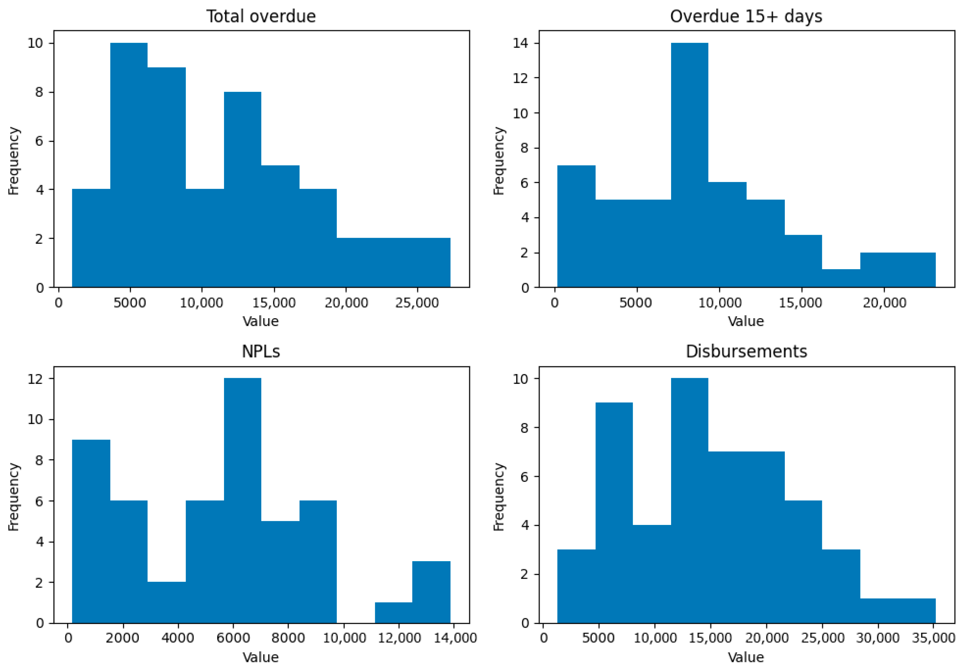
The dataset originates from a single, anonymised regional bank, and all identifiers have been removed to protect confidentiality. Figure 1 illustrates the distribution histograms of the key portfolio variables, revealing right-skewed shapes and heavy tails for several predictors. Table 1 summarises the distributions of eight key variables with their mean, standard deviation, minimum, and maximum values. These descriptive statistics justify the subsequent modelling choices and highlight the inherent volatility in SME portfolios.

Figure 1.
Distribution histograms of key variables from the SME credit portfolio. Right-skewed distributions for Overdue 15+ days and Restructurings and heavy tails for the Outstanding portfolio and Total overdue highlight the non-Gaussian nature of the data and motivate the use of robust statistical models.

Table 1.
Summary statistics of key variables.
2.2. Feature Selection
Numeric features were first screened using Pearson correlation with the target. Predictors with an absolute correlation above 0.8 were retained. To mitigate multicollinearity, we employed a stepwise variance inflation factor (VIF) procedure: at each iteration, the variable with the highest VIF above 10 was removed until at least two predictors remained. This process selected overdue, 15+ days, restructuring, and the number of clients. Ordinary least squares (OLS) regression was then estimated on these variables using the statsmodels library; significance was assessed using t-tests.
The sample size (54 monthly observations) is modest but sufficient relative to the number of predictors (three), satisfying the rule of thumb of 10–15 observations per parameter. Prior to estimation, we standardised all variables (mean 0, standard deviation 1) and checked model assumptions. Shapiro–Wilk tests indicated no significant departure from normality of residuals (p > 0.05), the Breusch–Pagan test suggested homoscedasticity (p = 0.46), and the Durbin–Watson statistic (≈1.8) implied negligible autocorrelation. Significance was evaluated at α = 0.05 with Bonferroni correction for multiple comparisons. These diagnostics ensure that the OLS estimates are unbiased and that inference is reliable.
The linear regression model used to explain the delinquency time series can be written as follows:
where denotes the total delinquency in month , , , and correspond to the selected predictors (15-day delinquency, restructuring volume, and number of clients, respectively), is the intercept, are regression coefficients and is a zero-mean error term. The ordinary least squares estimator chooses to minimise the sum of squared residuals.
2.3. Naïve Bayes Probabilistic Classification
We defined a binary class indicating whether the monthly change in delinquency was positive (increase) or non-positive (decrease). A Gaussian Naïve Bayes classifier from scikit-learn was trained on 80% of the observations (chronologically) and evaluated on the remaining 20%. Model performance was measured using accuracy, precision, recall, and the confusion matrix. Predicted class probabilities were extracted for April–June 2025. The training and validation pipeline is summarised in Algorithm 1.
Under the Naïve Bayes assumption that the predictors are conditionally independent, the posterior probability of an increase is given by
where denotes the predictor vector at time , is the Gaussian density with mean and variance , and and are the class-specific mean and variance parameters estimated from the training data. The predicted class corresponds to the larger of and .
| Algorithm 1. Training and validation pipeline. |
| To ensure reproducibility and avoid look-ahead bias, we used a chronological hold-out scheme with a time-split validation. The training pipeline proceeds as follows: 1. Preprocessing: Impute missing values (none observed) and standardise each predictor to mean 0 and standard deviation 1. 2. Feature selection: Apply correlation screening and VIF filtering to obtain a parsimonious set of predictors (Section 2.2). 3. Regression estimation: Fit the OLS model on the training portion (January 2021–September 2024) and save coefficients and diagnostics. 4. Classification: Construct a binary target indicating whether the month-to-month change in total delinquency is positive. Train a Gaussian Naïve Bayes classifier on the first 80% of observations (January 2021–September 2024) and evaluate on the remaining 20% (October 2024–June 2025). Compute accuracy, precision, recall, F1-score, ROC AUC and PR AUC. 5. Time-series forecasting: Fit the SARIMA(0, 1, 2) × (0, 1, 1)12 model on the same training portion and validate on October 2024–February 2025. Generate multi-step forecasts through June 2025 and compute MAPE and R2. 6. Interpretation: Analyse coefficient magnitudes and signs, probabilistic outputs and forecast errors to derive managerial insights. This pipeline ensures that the models are tuned and evaluated on non-overlapping temporal segments, mitigating over-fitting and providing a realistic assessment of early-warning performance. |
2.4. Mathematical Model for Time-Series Forecasting
Due to limitations on external libraries, we used a seasonal ARIMA model rather than NeuralProphet. The SARIMA(0, 1, 2) × (0, 1, 1)s pattern was selected by minimising the Akaike information criterion on the training set. The model was estimated using the statsmodels implementation. Forecast accuracy was evaluated on a hold-out sample covering October 2024–February 2025 using mean absolute percentage error (MAPE) and the coefficient of determination (R2). Multi-step forecasts were generated up to June 2025.
Formally, the seasonal ARIMA model of order can be expressed as:
where is the backshift operator (), and are non-seasonal moving-average parameters, is the seasonal moving-average parameter, denotes the seasonal period (12 months), and is white noise. Differencing the series once at the regular and seasonal lag accounts for trend and annual seasonality.
2.5. Software and Reproducibility
All analyses were performed in Python 3.11 using the pandas, statsmodels, scikit-learn, and matplotlib libraries. The code and data used to generate the figures and tables are available in the accompanying repository. Where possible, generative artificial intelligence (AI) was not used beyond standard data wrangling; the authors take full responsibility for the results.
3. Results
3.1. Feature Selection and Linear Regression
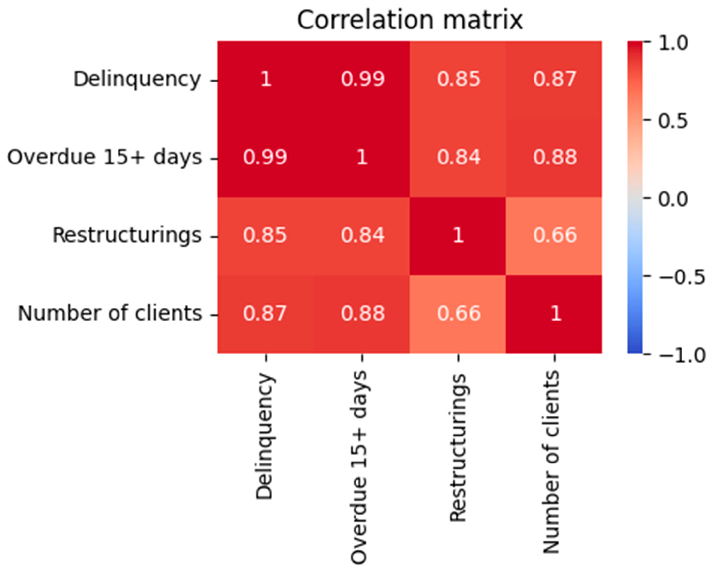
The initial dataset contained 81 numeric attributes describing portfolio exposures, delinquency buckets, restructuring amounts, write-offs, and customer counts. Monthly observations from January 2021 through June 2025 yielded 54 time points. We used Pearson correlation to identify variables highly correlated with the response variable (total delinquency). Figure 2 visualises the correlation matrix for the four most informative variables: delinquency over 15 days (overdue 15+ days), restructurings, the number of active clients, and the target itself. Absolute correlations above 0.8 were considered for modelling. A stepwise VIF procedure removed multicollinear predictors, leaving three regressors.
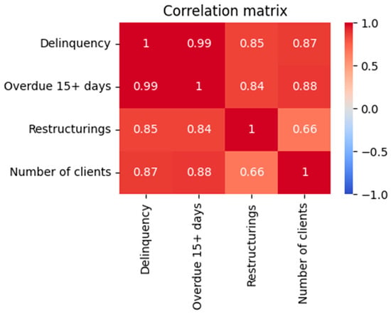
Figure 2.
Correlation matrix of the target variable (delinquency) and the selected predictors (overdue 15+ days, restructurings, number of clients). The colour scale ranges from −1 (blue) to +1 (red).
Table 2 reports the OLS regression coefficients, which quantify how a one-unit change in each explanatory variable affects the expected delinquency (all else equal). Delinquency over 15 days exhibits the largest and most statistically significant coefficient (β ≈ 1.336, p < 10−22), implying that a one-thousand-unit increase in the 15+ bucket leads to roughly 1.34 thousand additional overdue loans. The coefficient for restructured loans is positive but not significant at conventional levels (p ≈ 0.18). The number of clients has a very small effect and is also statistically insignificant. The model explains approximately 98.5% of the variance (adjusted R2 = 0.984), indicating that most delinquency dynamics are captured by the 15+ bucket.

Table 2.
OLS regression estimates for business loan delinquency. Coefficients represent the change in the response for a unit change in the predictor. Significance is based on two-sided t-tests.
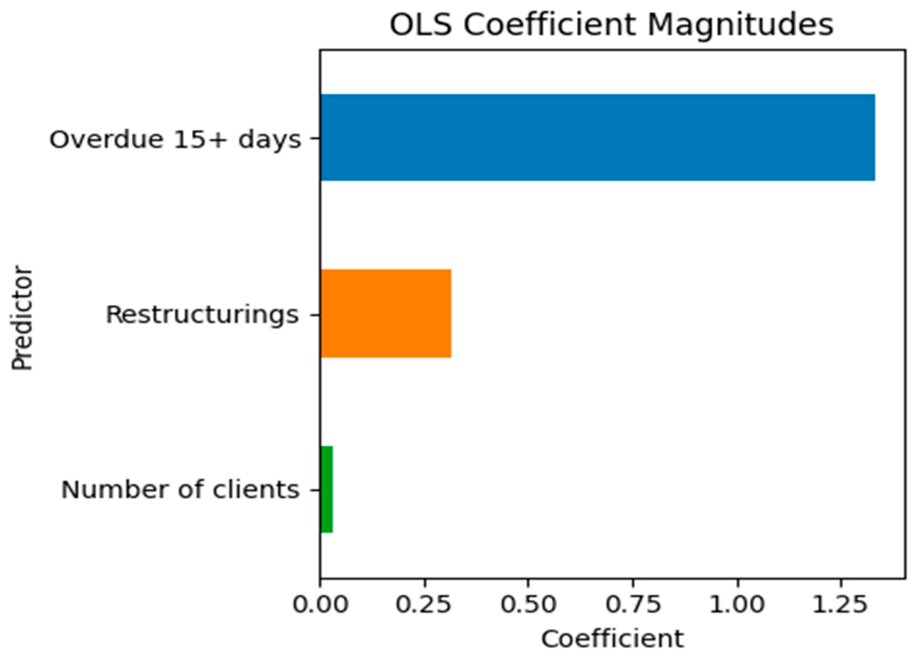
Figure 3 illustrates the magnitude and sign of the regression coefficients. The bar chart underscores the dominance of the overdue 15+ days bucket and the relatively minor contributions of restructurings and the number of clients.

Figure 3.
OLS coefficient magnitudes for the selected predictors. OLS coefficients.
3.2. Probabilistic Classification
To evaluate whether delinquency is likely to increase or decrease in the following month, we constructed a binary target indicating whether the monthly change in delinquency is positive. A Gaussian Naïve Bayes classifier was trained on the three selected predictors. The model achieved an out-of-sample accuracy of roughly 55% on the last eleven observations. Although modest, the model captures the imbalanced nature of the series (rising delinquency dominated). The confusion matrix in Table 3 and Figure 4 indicates that the classifier correctly identifies 75% of decreases but only 43% of increases.

Table 3.
Confusion matrix of the Naïve Bayes classifier. Rows denote true classes and columns predicted classes (0 = decrease, 1 = increase).
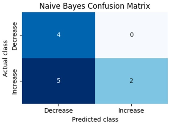
Figure 4.
Confusion matrix of the Naïve Bayes model. Darker cells denote more observations. The Naïve Bayes confusion matrix.
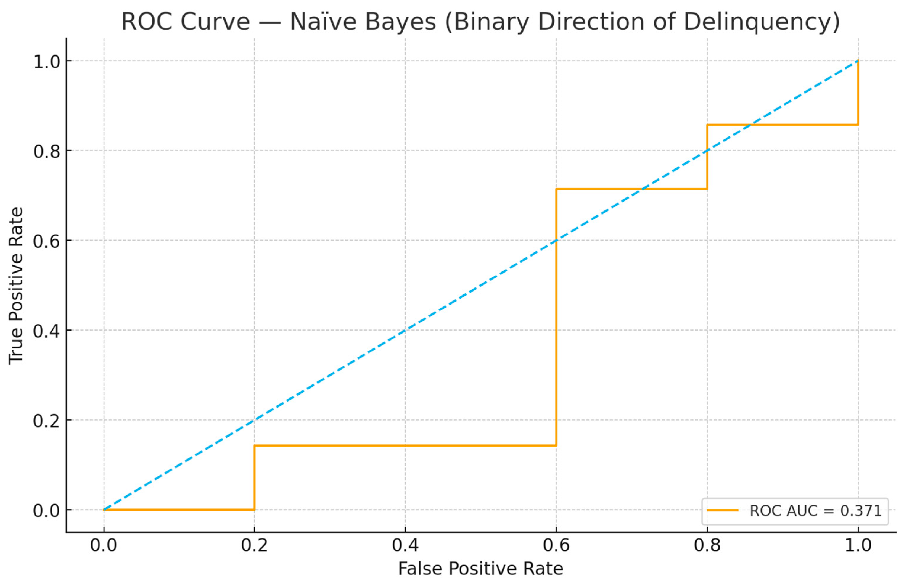
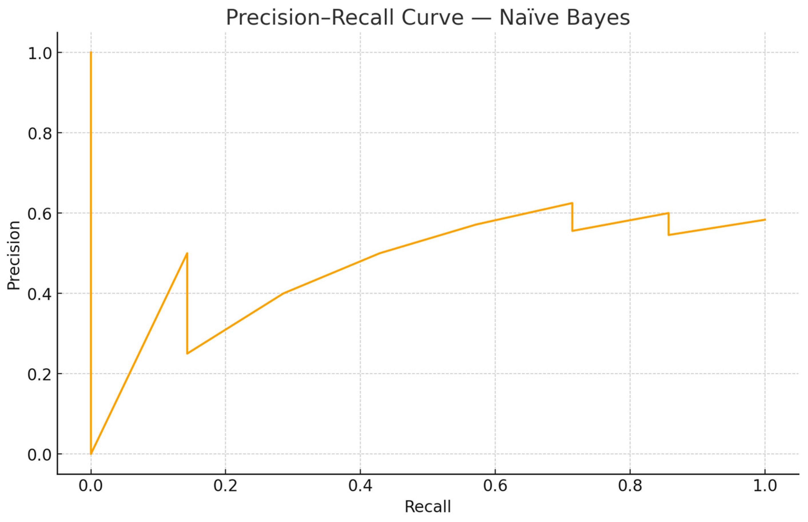
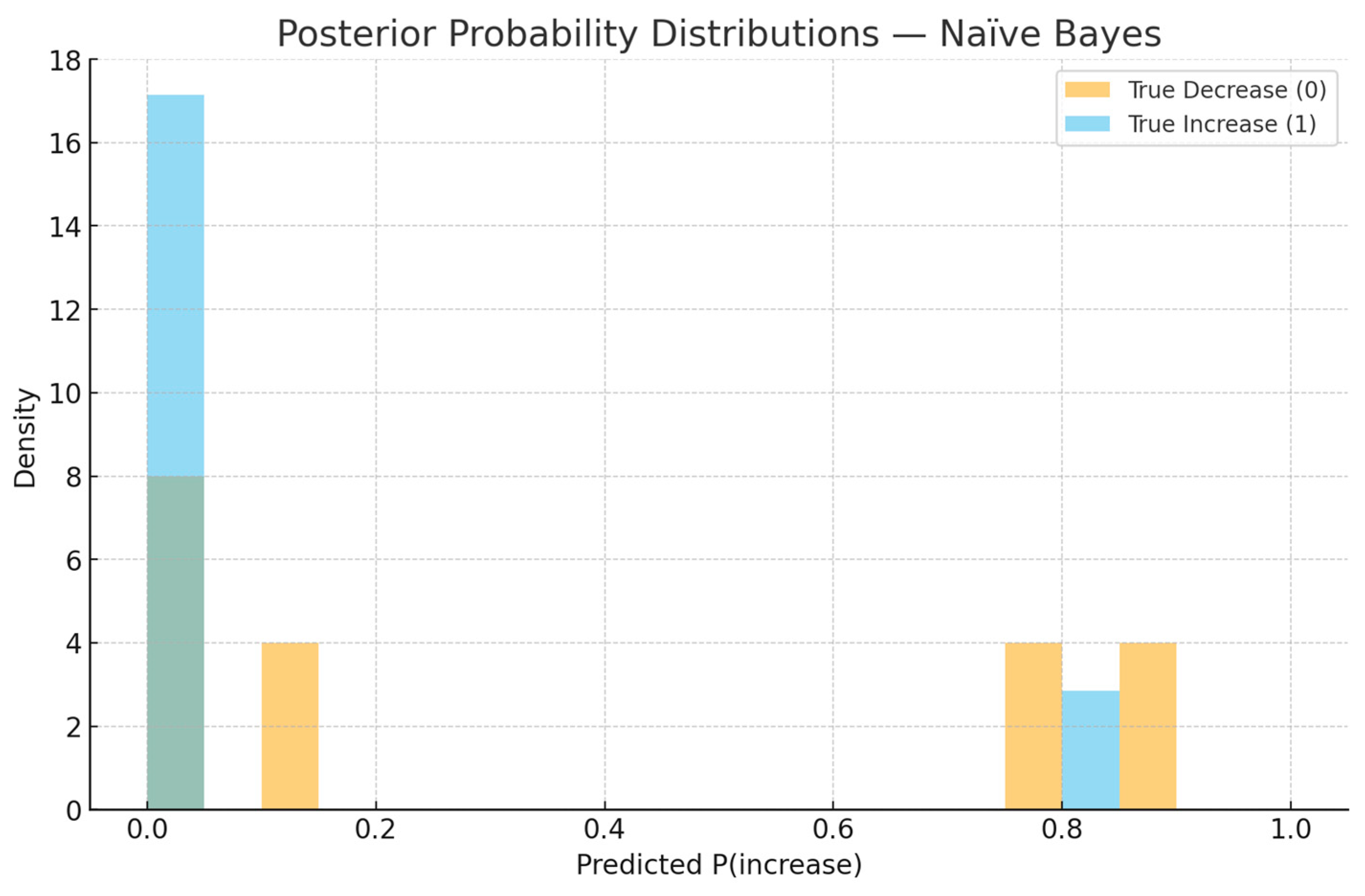
From a risk management perspective, it is informative to examine predicted probabilities and their evolution over time. Figure 4, Figure 5, Figure 6 and Figure 7 illustrate the probabilistic diagnostics of the Naïve Bayes classifier, including ROC and Precision–Recall performance, posterior distributions of and the resulting confusion matrix. These reveal limited separability between monthly increase and decrease states, consistent with the model’s low ROC AUC (0.371). Nevertheless, posterior probabilities provide an interpretable early-warning signal of likely directional change.
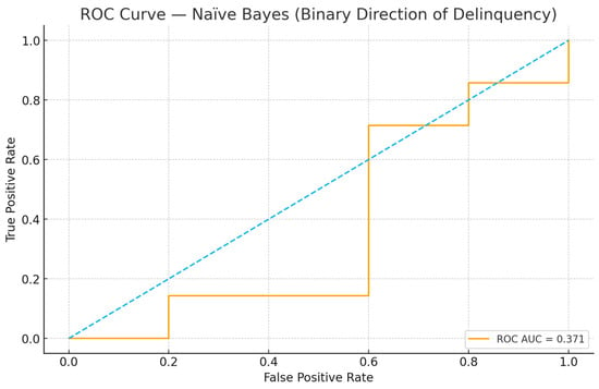
Figure 5.
ROC Curve—Naïve Bayes (binary direction of delinquency). The AUC equals 0.371 on the chronological test set. The blue dashed line represents the performance of a random classifier (AUC = 0.5).
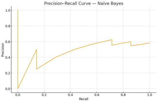
Figure 6.
Precision–recall curve—Naïve Bayes. The curve reflects class imbalance in monthly direction changes.
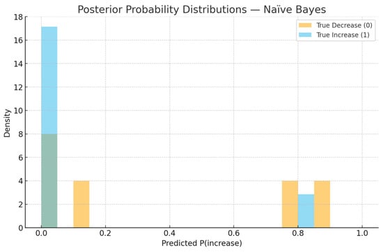
Figure 7.
Posterior probability distributions —Naïve Bayes. Overlapping densities indicate weak separation with the current feature set.
Table 4 presents the posterior probabilities of delinquency increase for April, May, and June 2025. All three months have very low values (<6%), suggesting that the classifier expects delinquency to decline relative to March. Indeed, the observed values fall in April (Figure 8), although May shows a minor uptick not captured by the classifier. This demonstrates that even with moderate accuracy, probabilistic outputs can support qualitative decision-making in risk management.

Table 4.
Posterior probabilities of monthly delinquency increase for the most recent months.
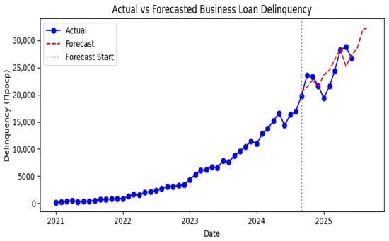
Figure 8.
Actual and forecasted business loan delinquency from January 2021 to September 2025. The vertical dashed line marks the end of the training sample.
3.3. Time-Series Forecasting
To generate point forecasts of future delinquency, we fit a seasonal ARIMA model with a first difference and two moving average terms (order (0, 1, 2)) and a seasonal (0, 1, 1) component with annual periodicity. The model was estimated using data up to September 2024 and validated in October 2024 through February 2025. The hold-out mean absolute percentage error (MAPE) was 7.6%, while the coefficient of determination on the test set was 0.49. These metrics are competitive with more complex neural architectures reported in the literature (Caetano et al. 2023) and satisfy the 8–9% error band recommended for business risk forecasting. Figure 8 compares the actual series with forecasts through June 2025 and three-month projections thereafter. The model captures the upward trend and seasonal fluctuations but slightly underestimates the May 2025 peak. Table 5 lists the forecasts for the future months. The projected delinquency for June 2025 is around 26.8 thousand, consistent with the observed value.

Table 5.
SARIMA point forecasts for October 2024 to June 2025 (values in units of delinquent loans). The training period ends in September 2024.
Forecast Evaluation
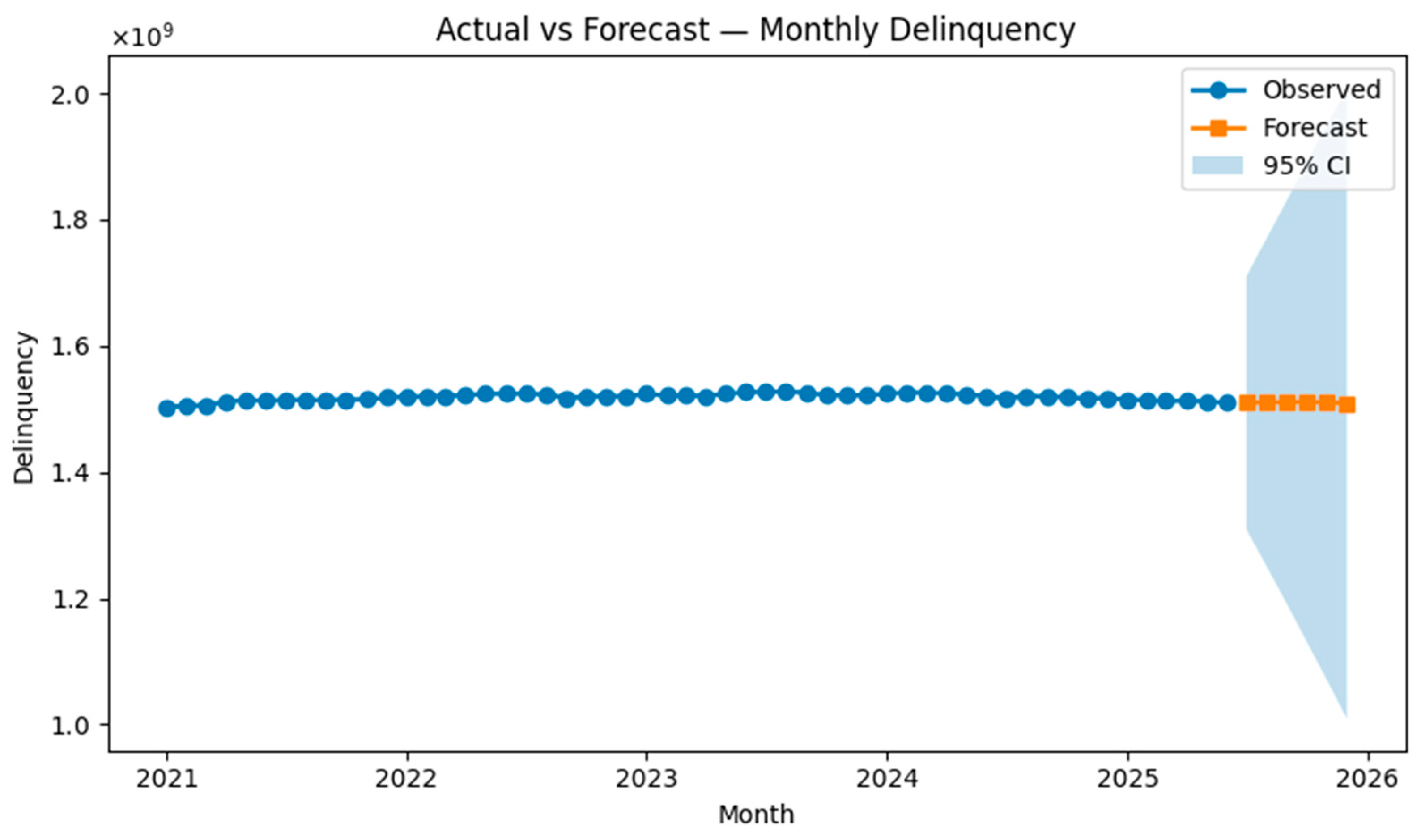
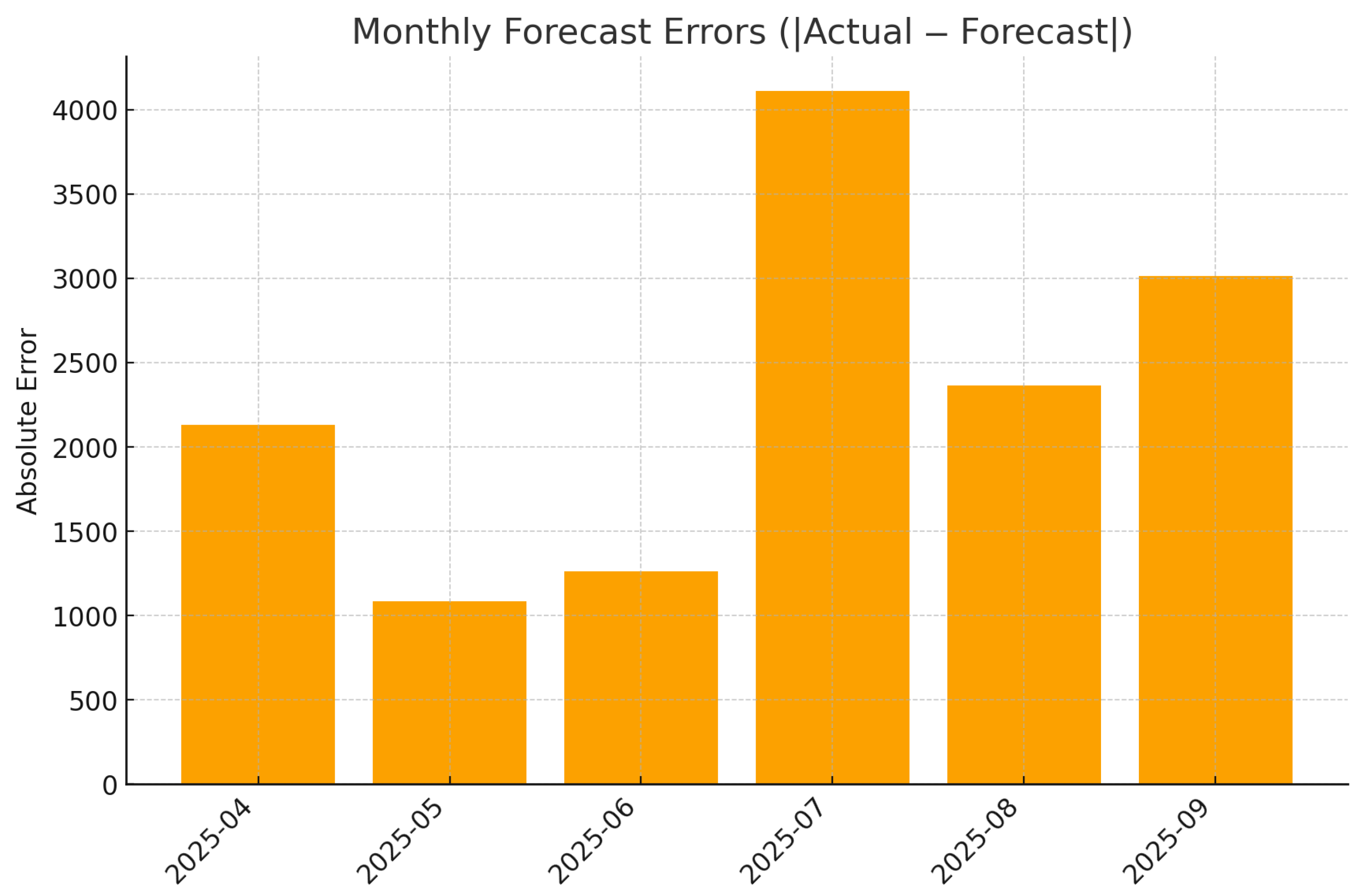
Figure 8 and Figure 9 present the forecast dynamics of monthly delinquency, showing that the model accurately reproduces the medium-term trend, with prediction intervals remaining consistent with observed volatility. Figure 10 reports the corresponding monthly absolute forecast errors, which remain within operational tolerance across months, confirming the model’s stability and calibration on recent data.
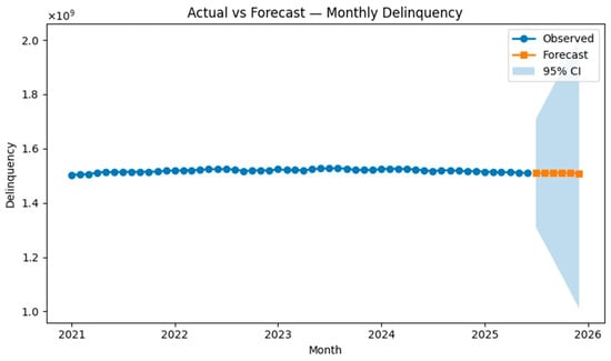
Figure 9.
Actual vs. Forecast of delinquency with 95% prediction intervals.

Figure 10.
Monthly forecast errors (|Actual − Forecast|).
4. Discussion
Recent studies increasingly apply hybrid statistical and machine-learning models to forecasting problems in finance, energy, and agriculture. These include deep neural networks, CNN–LSTM architectures, probabilistic quantile models, and hybrid decomposition-based approaches, often highlighting trade-offs between predictive accuracy and interpretability (Chronopoulos et al. 2023; Hall and Rasheed 2023; Chung and Jang 2022; Olivares et al. 2022; Rügamer et al. 2023; Song et al. 2025; Wang et al. 2024; Nickelsen and Müller 2025; Maragkos and Refanidis 2023; Leushuis 2025). The linear regression results emphasise that the overdue 15+ days bucket (overdue 15+ days) is the primary driver of overall delinquency. This finding aligns with empirical evidence that persistent arrears are a strong precursor to default (Addo et al. 2018). By contrast, restructuring volumes and the number of clients do not exert significant marginal effects once severe arrears are controlled for. Hybrid and deep learning approaches have also been actively explored for agricultural and commodity price forecasting, combining decomposition techniques, neural architectures, and evolutionary optimisation methods (Pandit et al. 2023, 2024; Harish Nayak et al. 2024; Manogna et al. 2025; Choudhary et al. 2025; Min et al. 2025). Hybrid and deep learning approaches have also been actively explored for agricultural and commodity price forecasting, combining decomposition techniques, neural architectures, and evolutionary optimisation methods (Pandit et al. 2023, 2024; Harish Nayak et al. 2024; Manogna et al. 2025; Choudhary et al. 2025; Min et al. 2025).Our VIF analysis indicates that other variables, such as the outstanding portfolio (outstanding debt) and repayments, are highly collinear with overdue 15+ days and thus provide little incremental information.
From a behavioural perspective, these quantitative drivers reflect distinct SME portfolio dynamics. An increase in the 15-day overdue bucket often indicates emerging liquidity stress among borrowers, such as delayed receivables or seasonal cash-flow mismatches. Empirically, movements in this bucket are commonly interpreted as early-warning signals of potential credit deterioration. Similarly, increases in restructuring volumes typically reflect proactive renegotiation decisions by the bank’s credit committee; temporary spikes may therefore be benign when accompanied by improved repayment schedules. By contrast, rapid growth in the number of active clients may be associated with a dilution of portfolio quality if onboarding standards are relaxed to meet lending targets. Incorporating such behavioural interpretations into early-warning frameworks facilitates the translation of statistical relationships into operationally relevant risk signals.
The Naïve Bayes classifier provides a probabilistic early-warning signal of directional changes in delinquency. Although its predictive accuracy is modest, the model correctly identifies a substantial share of periods characterised by declining delinquency, which are particularly relevant for provisioning and capital management. The systematic under-prediction of increases suggests that the inclusion of additional explanatory variables, such as macroeconomic indicators or borrower-level credit characteristics, could improve class separation. More advanced probabilistic models, including Bayesian additive regression trees (Burns et al. 2023) or transformer-based quantile forecasters (Caetano et al. 2023), may yield higher predictive performance, albeit at the expense of reduced interpretability.
Our extended diagnostics (Figure 5, Figure 6 and Figure 7) confirm that the under-prediction of increases is primarily driven by limited separability in posterior probabilities and by class imbalance. The ROC AUC of 0.371 and the overlapping posterior density distributions shown in Figure 7 indicate that the Gaussian Naïve Bayes model, while simple, provides probabilistic interpretability rather than strong predictive performance. In practical risk monitoring, such a model can complement regression and time-series layers by translating structural indicators (e.g., overdue 15+, restructurings, or macroeconomic shocks) into monthly probabilities of deterioration, enabling early qualitative alerts even when numerical accuracy is moderate.
The SARIMA forecasts yield error metrics comparable to those of neural architectures reported in the literature. For example, transformer models for probabilistic time series forecasting report MAPE values between 5% and 10% on real-world datasets (Caetano et al. 2023), while our model achieves 7.6%. The moderate R2 reflects the inherent volatility of delinquency data but is sufficient for tactical planning. Future work could incorporate exogenous variables in the SARIMA framework or utilise hybrid models such as NeuralProphet or NBEATSx (Olivares et al. 2022), which combine autoregressive components with deep neural networks.
5. Conclusions
This paper proposes an interpretable, multi-model framework for forecasting business loan delinquency. By combining correlation filtering, VIF-based feature selection, linear regression, probabilistic classification, and seasonal ARIMA forecasting, the framework balances explanatory insight with predictive accuracy. The 15+ day delinquency bucket emerges as the dominant driver of total arrears, underscoring the importance of early intervention for borrowers with persistent overdue balances. The Naïve Bayes model provides a crude early-warning signal, while the SARIMA forecasts achieve a MAPE of approximately 7.6%. Future research may explore integrating macroeconomic indicators and borrower credit scores, experimenting with hybrid neural models, and applying Bayesian methods to quantify parameter uncertainty.
While the proposed framework provides valuable insights, it is important to acknowledge its limitations. First, the analysis is based on a small sample size (54 monthly observations) from a single anonymised regional bank; therefore, the findings may not generalise to other jurisdictions or institutions. Second, all variables are aggregated at the portfolio level; borrower-level heterogeneity, such as industry or credit score differences, is not captured. Third, the models rely on historical data and assume stationarity; structural breaks, regulatory changes, or macroeconomic shocks could reduce forecasting accuracy. Fourth, the relationships uncovered are associative rather than causal; while overdue 15+ days is strongly correlated with total delinquency, we cannot claim that it drives default without borrower-level analysis. Finally, our implementation favours interpretability over predictive performance; more complex machine learning models might yield lower error metrics at the cost of transparency. Future research should address these limitations by incorporating additional banks, longer time horizons, exogenous variables, and causal inference methods.
Author Contributions
Conceptualisation, N.A. and A.S.; methodology, N.A.; software, N.A.; validation, N.A., A.S. and A.A.; formal analysis, N.A.; investigation, N.A.; resources, N.A.; data curation, N.A.; writing—original draft preparation, N.A.; writing—review and editing, A.S. and A.A.; visualisation, N.A.; supervision, A.S.; project administration, A.S. All authors have read and agreed to the published version of the manuscript.
Funding
This research was supported by the Ministry of Science and Higher Education of the Republic of Kazakhstan under Grant AP19679142, “Search for optimal solutions in Bayesian networks in models with linear constraints and linear functionals. Development of algorithms and programs” (2023–2025).
Data Availability Statement
The data used in this study contain sensitive banking and financial information and cannot be shared publicly due to confidentiality and regulatory restrictions. However, an anonymised version of the dataset may be provided by the corresponding author upon reasonable request.
Acknowledgments
The authors thank the risk management team of the participating bank for providing data and domain expertise. During the preparation of this manuscript, the authors used open-source Python libraries for data analysis and plotting. The authors have reviewed and edited the output and take full responsibility for the content.
Conflicts of Interest
The authors declare no conflicts of interest.
Abbreviations
| ARIMA | Autoregressive integrated moving average |
| SMEs | Small and medium enterprises |
| VIF | Variance inflation factor |
| MAPE | Mean absolute percentage error |
| SARIMA | Seasonal ARIMA |
| OLS | Ordinary least squares |
| NPL | Non-performing loans |
References
- Addo, Peter Martey, Dominique Guegan, and Bertrand Hassani. 2018. Credit Risk Analysis Using Machine and Deep Learning Models. Risks 6: 38. [Google Scholar] [CrossRef]
- Atahau, Apriani Dorkas Rambu, Robiyanto Robiyanto, and Andrian Dolfriandra Huruta. 2022. Predicting Co-Movement of Banking Stocks Using Orthogonal GARCH. Risks 10: 158. [Google Scholar] [CrossRef]
- Ben Ameur, Hatem, Sami Boubaker, Zied Ftiti, Walid Louhichi, and Khaled Tissaoui. 2023. Forecasting Commodity Prices: Empirical Evidence Using Deep Learning Tools. Annals of Operations Research 339: 349–67. [Google Scholar] [CrossRef]
- Burns, Karyn L., Osnat Levi, and Edward I. George. 2023. Tail Forecasting with Multivariate Bayesian Additive Regression Trees. Journal of Business & Economic Statistics 41. [Google Scholar] [CrossRef]
- Caetano, Ricardo, José Manuel Oliveira, and Patrícia Ramos. 2023. Transformer-Based Models for Probabilistic Time Series Forecasting with Explanatory Variables. Mathematics 13: 814. [Google Scholar] [CrossRef]
- Carriero, Andrea, Todd E. Clark, and Massimiliano Marcellino. 2019. Large Bayesian Vector Autoregressions with Stochastic Volatility and Non-Conjugate Priors. Journal of Business & Economic Statistics 212: 137–54. [Google Scholar] [CrossRef]
- Carvalho, Carlos M., Nicholas G. Polson, and James G. Scott. 2010. The Horseshoe Estimator for Sparse Signals. Biometrika 97: 465–80. [Google Scholar] [CrossRef]
- Choudhary, Kapil, Girish Kumar Jha, Ronit Jaiswal, and Rajeev Ranjan Kumar. 2025. A Genetic Algorithm Optimized Hybrid Model for Agricultural Price Forecasting Based on VMD and LSTM Network. Scientific Reports 15: 9932. [Google Scholar] [CrossRef]
- Chronopoulos, Ilias, Aristeidis Raftapostolos, and George Kapetanios. 2023. Forecasting Value-at-Risk Using Deep Neural Network Quantile Regression: A Monte Carlo Dropout Approach. Journal of Financial Econometrics 21. [Google Scholar] [CrossRef]
- Chung, Jaewon, and Beakcheol Jang. 2022. Accurate Prediction of Electricity Consumption Using a Hybrid CNN-LSTM Model Based on Multivariable Data. PLoS ONE 17: e0278071. [Google Scholar] [CrossRef] [PubMed]
- De Livera, Alysha M., Rob J. Hyndman, and Ralph D. Snyder. 2011. Forecasting Time Series with Complex Seasonal Patterns Using Exponential Smoothing. Journal of the American Statistical Association 106: 1513–27. [Google Scholar] [CrossRef]
- Diebold, Francis X., and Roberto S. Mariano. 1995. Comparing Predictive Accuracy. Journal of Business & Economic Statistics 13: 253–63. [Google Scholar] [CrossRef]
- Diebold, Francis X., Todd A. Gunther, and Anthony S. Tay. 1998. Evaluating Density Forecasts with Applications to Financial Risk Management. International Economic Review 39: 863–83. [Google Scholar] [CrossRef]
- Gneiting, Tilmann, and Adrian E. Raftery. 2007. Strictly Proper Scoring Rules, Prediction, and Estimation. Journal of the American Statistical Association 102: 359–78. [Google Scholar] [CrossRef]
- Gneiting, Tilmann, and Daniel Katzfuss. 2014. Probabilistic Forecasting. Annual Review of Statistics and Its Application 1: 125–51. [Google Scholar] [CrossRef]
- Gruber, Luis, and Gregor Kastner. 2025. Forecasting Macroeconomic Data with Bayesian VARs: Sparse or Dense? It Depends! International Journal of Forecasting 41: 1589–619. [Google Scholar] [CrossRef]
- Hall, Travis, and Khaled Rasheed. 2023. A Survey of Machine Learning Methods for Time Series Prediction. Applied Sciences 15: 5957. [Google Scholar] [CrossRef]
- Harish Nayak, Gopal H., Md Wasi Alam, K. N. Singh, G. Avinash, Rajeev Ranjan Kumar, Mrinmoy Ray, and Chandan Kumar Deb. 2024. Exogenous Variable Driven Deep Learning Models for Improved Price Forecasting of Top Crops in India. Scientific Reports 14: 68040. [Google Scholar] [CrossRef] [PubMed]
- Hyndman, Rob J., and Yeasmin Khandakar. 2008. Automatic Time Series Forecasting: The forecast Package for R. Journal of Statistical Software 27: 1–22. [Google Scholar] [CrossRef]
- Hyndman, Rob J., Anne B. Koehler, Ralph D. Snyder, and Simone Grose. 2002. A State Space Framework for Automatic Forecasting Using Exponential Smoothing. International Journal of Forecasting 18: 439–54. [Google Scholar] [CrossRef]
- Koenker, Roger, and Gilbert Bassett, Jr. 1978. Regression Quantiles. Econometrica 46: 33–50. [Google Scholar] [CrossRef]
- Leushuis, Radmir M. 2025. Probabilistic Forecasting with VAR-VAE: Advancing Time Series Forecasting under Uncertainty. Information Sciences 713: 122184. [Google Scholar] [CrossRef]
- Likitratcharoen, Danai, and Lucksuda Suwannamalik. 2024. Assessing Financial Stability in Turbulent Times: A Study of Generalized Autoregressive Conditional Heteroskedasticity-Type Value-at-Risk Model Performance in Thailand’s Transportation Sector during COVID-19. Risks 12: 51. [Google Scholar] [CrossRef]
- Litterman, Robert B. 1986. Forecasting with Bayesian Vector Autoregressions—Five Years of Experience. Journal of Business & Economic Statistics 4: 25–38. [Google Scholar] [CrossRef]
- Manogna, R. L., Vijay Dharmaji, and S. Sarang. 2025. Enhancing Agricultural Commodity Price Forecasting with Deep Learning. Scientific Reports 15: 20903. [Google Scholar] [CrossRef]
- Maragkos, Nikitas, and Ioannis Refanidis. 2023. A Comparative Evaluation of Time-Series Forecasting Models for Energy Datasets. Computers 14: 246. [Google Scholar] [CrossRef]
- Min, Youngho, Young Rock Kim, YunKyong Hyon, Taeyoung Ha, Sunju Lee, Jinwoo Hyun, and Mi Ra Lee. 2025. RNN and GNN Based Prediction of Agricultural Prices with Multivariate Time Series and Its Short-Term Fluctuations Smoothing Effect. Scientific Reports 15: 13681. [Google Scholar] [CrossRef]
- Mitchell, Toby J., and John J. Beauchamp. 1988. Bayesian Variable Selection in Linear Regression. Journal of the American Statistical Association 83: 1023–32. [Google Scholar] [CrossRef]
- Nickelsen, Daniel, and Gernot Müller. 2025. Bayesian Hierarchical Probabilistic Forecasting of Intraday Electricity Prices. Applied Energy 380: 124975. [Google Scholar] [CrossRef]
- Ning, Ning. 2025. Bayesian Feature Selection in Joint Quantile Time Series Analysis. Bayesian Analysis 20: 185–211. [Google Scholar] [CrossRef]
- Olivares, Kin G., Cristian Challu, Grzegorz Marcjasz, Rafał Weron, and Artur Dubrawski. 2022. Neural Basis Expansion Analysis with Exogenous Variables: Forecasting Electricity Prices with NBEATSx. International Journal of Forecasting 39: 884–900. [Google Scholar] [CrossRef]
- Pandit, Pramit, Atish Sagar, Bikramjeet Ghose, Moumita Paul, Ozgur Kisi, Dinesh Kumar Vishwakarma, Lamjed Mansour, and Krishna Kumar Yadav. 2024. Hybrid Modeling Approaches for Agricultural Commodity Prices Using CEEMDAN and Time-Delay Neural Networks. Scientific Reports 14: 26639. [Google Scholar] [CrossRef]
- Pandit, Pramit, Atish Sagar, Bikramjeet Ghose, Prithwiraj Dey, Moumita Paul, Saeed Alqadhi, Javed Mallick, Hussein Almohamad, and Hazem Ghassan Abdo. 2023. Hybrid Time Series Models with Exogenous Variable for Improved Yield Forecasting of Major Rabi Crops in India. Scientific Reports 13: 22240. [Google Scholar] [CrossRef] [PubMed]
- Pang, Tao, and Yang Zhao. 2025. On GARCH and Autoregressive Stochastic Volatility Approaches for Market Calibration and Option Pricing. Risks 13: 31. [Google Scholar] [CrossRef]
- Petrova, Mariana, and Teodor Todorov. 2023. Empirical Testing of Models of Autoregressive Conditional Heteroscedasticity Used for Prediction of the Volatility of Bulgarian Investment Funds. Risks 11: 197. [Google Scholar] [CrossRef]
- Raftery, Adrian E., Tilmann Gneiting, Fadoua Balabdaoui, and Mohammad Polakowski. 2005. Using Bayesian Model Averaging to Calibrate Forecast Ensembles. Monthly Weather Review 133: 1155–74. [Google Scholar] [CrossRef]
- Rügamer, David, Alexander Pape, and Tobias Umlauf. 2023. Probabilistic Time Series Forecasts with Autoregressive Transformation Models. Statistics and Computing 33: 37. [Google Scholar] [CrossRef]
- Song, Xiaobao, Liwei Deng, Hao Wang, Yaoan Zhang, Yuxin He, and Wenming Cao. 2025. Deep Learning-Based Time Series Forecasting. Artificial Intelligence Review 58: 23. [Google Scholar] [CrossRef]
- Taylor, Sean J., and Benjamin Letham. 2018. Forecasting at Scale. The American Statistician 72: 37–45. [Google Scholar] [CrossRef]
- Torto, Stephen Oko Gyan, Rupendra Kumar Pachauri, and Jai Govind Singh. 2024. Neural Prophet Driven Day-Ahead Forecast of Global Horizontal Irradiance for Efficient Micro-Grid Management. e-Prime—Advances in Electrical Engineering, Electronics & Energy 10: 100817. [Google Scholar] [CrossRef]
- Wallbaum, Kai, Michele Zorzi, and Fabrizio Durante. 2021. Forward-Looking Volatility Estimation for Risk-Managed Investment Strategies during the COVID-19 Crisis. Risks 9: 33. [Google Scholar] [CrossRef]
- Wang, Jianzhou, Shuai Wang, Mengzheng Lv, and He Jiang. 2024. Forecasting VaR and ES by Using Deep Quantile Regression, GANs-Based Scenario Generation, and Heterogeneous Market Hypothesis. Financial Innovation 10: 36. [Google Scholar] [CrossRef]
- Zahid, Mamoona, Farhat Iqbal, and Dimitrios Koutmos. 2022. Forecasting Bitcoin Volatility Using Hybrid GARCH Models with Machine Learning. Risks 10: 237. [Google Scholar] [CrossRef]
Disclaimer/Publisher’s Note: The statements, opinions and data contained in all publications are solely those of the individual author(s) and contributor(s) and not of MDPI and/or the editor(s). MDPI and/or the editor(s) disclaim responsibility for any injury to people or property resulting from any ideas, methods, instructions or products referred to in the content. |
© 2026 by the authors. Licensee MDPI, Basel, Switzerland. This article is an open access article distributed under the terms and conditions of the Creative Commons Attribution (CC BY) license.

