Abstract
This paper investigates the optimal asset allocation of a financial institution whose customers are free to withdraw their capital-guaranteed financial contracts at any time. In accounting for the asset-liability mismatch risk of the institution, we present a general utility optimization problem in a discrete-time setting and provide a dynamic programming principle for the optimal investment strategies. Furthermore, we consider an explicit context, including liquidity risk, interest rate, and credit intensity fluctuations, and show by numerical results that the optimal strategy improves both the solvency and asset returns of the institution compared to a standard institutional investor’s asset allocation.
1. Introduction
Recent financial turmoil and market stresses following the sub-prime crisis or the COVID-19 pandemic had a double impact on asset management: massive withdrawals accompanied by violent and persistent liquidity shocks. This type of phenomenon constitutes a major risk for financial institutions including banks, insurers, and pension funds that offer capital-guaranteed contracts, such as deposit accounts or life insurance savings products, as it can lead to the bankruptcy of the institution.
Capital-guaranteed contracts are characterized by the security of the capital invested, the absence of predetermined maturity, and the right of customers to surrender it at any time. The sharp increase in redemptions generally occurs in two main cases: (i) when customers consider the financial institution to be at risk, usually during a financial crisis when default risk increases; or (ii) when customers find more attractive investment opportunities, usually during periods of rising interest rates. It becomes difficult for a financial institution to meet its redemptions when it is concomitantly exposed to a liquidity shock that forces it to sell assets at discounted prices. This situation deteriorates the solvency of the financial institution that bears the guaranteed-capital risk, which increases the demand for redemptions and can induce a snowball effect, leading to the insolvency of the institution.
The negative impact of these forced sales at a discounted price on the institution’s solvency can materialize in several ways. First, they decrease the amount of free surplus available and hence the institution’s solvency, as the value of the asset decreases. Indeed, Cao and Petrasek (2014) showed that abnormal stock returns during liquidity crises are strongly negatively related to liquidity risk and evidence from Favero et al. (2009) showed that the government bond yields a hike when the liquidity of the securities declines in a more pronounced way on long-dated bonds (Goyenko et al. 2010). Moreover, as shown by Goyenko and Ukhov (2009), illiquidity shocks spill over from stocks to bonds (notably via flight-to-quality) and reciprocally since it is the channel through which monetary policy shocks impact the stock market. Furthermore, when the stress is accompanied by a decrease in the rating of the security, as supported by evidence from Chen et al. (2011) that an increase in corporate internal liquidity risk hikes credit risk, this weighs on the cost of capital and thus, again, on the institution’s solvency. In addition, as the asset prices decrease, they are fueled by a ricochet effect via the unwinding of positions (Allen and Gale 2004) and via margin calls that increase the downward spiral (Brunnermeier and Pedersen 2008).
The solvency risk implied by a liquidity mismatch between the assets and liabilities of a financial institution has increased in the recent years for two reasons. First, institutional investors are not legally required to build a sufficient cushion to absorb the liquidity risk. For instance, the Solvency II Directive does not require regulatory capital (Solvency Capital Requirement) to be based on the illiquidity of assets held by European insurers. Yet, this major risk is taken into account for investment funds: the European Securities and Markets Authority recently published a set of guidelines on liquidity stress testing to be implemented from 1 September 2020. Second, the low interest rate environment that has prevailed since the end of the sub-prime and sovereign debt crises has incentivized financial institutions in a yield-seeking race, leading to significant investments in illiquid assets.
This paper first investigates, in a fairly general framework, the optimal asset allocation of a financial institution offering capital-guaranteed contracts and whose customers are free to withdraw their financial contract at any time on the liability side. We suppose that the withdrawals occur according to a general marked point process whose jump times represent the surrender times from the customers and random marks represent the payment values of each withdrawal. The intensity of the point process, which characterizes the frequency of withdrawals, may typically be impacted by the uncertainty of the rise of interest rates and the deterioration of credit quality. We consider a discrete time setting where the transactions take place at a finite set of discrete times to be consistent with the effective practices of asset managers. The financial institution, given its risk aversion, searches to optimize the asset allocation of the investment portfolio by using the expected utility maximization upon the wealth value at a final horizon. Moreover, several solvency constraints are specified to impose asset-liability requirements in terms of risk measures, such as the quantile and the expected shortfall introduced by Föllmer and Leukert (1999, 2000). In literature, portfolio management with benchmarking and constraints has been studied to find the so-called Desired Benchmark Strategy; see, for example, Boyle and Tian (2007), with a quantile constraint outperforming a stochastic benchmark at final time, Gundel and Weber (2007), with a joint expected shortfall and budget constraint, or El Karoui et al. (2005), with a deterministic benchmark at all future dates.
In our paper, the solvency risk is examined with a stochastic liability, which represents the guaranteed-capital level. Moreover, the asset-liability constraints are required in a dynamic way at each time step. We may also include the constraint at the final time as a penalty added to the utility function. In order to study these constraints of different nature in a coherent way, we adopt the random utility as in Blanchard and Carassus (2018), which allows us to incorporate the penalized utility depending on an extra random element. We provide a dynamic programming principle for the general optimization problem. The main technical point is to prove that the admissible trading strategy set under all the required constraints remains stable by El Karoui (1981). Then, the optimal dynamic investment strategy can be obtained recursively. For the exponential utility function, the optimal value function at each time step remains as a weighted exponential function. For the power utility function, an explicit form of the optimal value function is more difficult to derive. In this case, we obtain the solution by numerical methods.
The financial institution can invest in interest rate and credit, and therefore it is exposed to these market risks. In a subsequent step, we consider a special portfolio subject to withdrawal and liquidity risks under credit intensity and interest rate fluctuation. Financial liquidity risk increase has been materialized notably in an increase of investments in high yield bonds (Bao et al. 2011; Dick-Nielsen et al. 2012). While some assets can be clearly identified as specifically illiquid, many liquid assets can become illiquid in times of financial stress. In considering bonds, Favero et al. (2009) and Chen et al. (2011) show that a rise in government or corporate internal liquidity risk increases credit risk, which further deteriorates the solvency of the institution. Similarly as in Chen et al. (2017), we suppose that the liquidity intensity increases with the credit risk. More precisely, the intensity of liquidity shocks is supposed to be a CEV function (see, e.g., Carr and Linetsky (2006)) of the credit intensity. In line with practice and the literature, the institution optimizes its solvency over a given horizon (Berry-Stölzle 2008; Cousin et al. 2016; Pan and Xiao 2017) and the optimal strategies are illustrated by numerical resolution using the methodology introduced in Brandt et al. (2005) as well as by the calibration of market data for interest rate and credit intensity. We show how accounting for the joint risks of liquidity on the assets side and withdrawals on the liabilities side substantially modifies the optimal asset allocation and that the latter outperforms standard allocations in terms of the solvency ratio and asset returns. Specifically, we show how the increase in credit and interest rate risks pushes the financial institution to secure its allocation, thereby mitigating its default risk.
Our contribution to the literature on optimal asset allocation and asset-liability management is twofold. First, we introduce an endogenous withdrawal risk, which affects both the assets portfolio and the liability benchmark. The solvency constraints are examined in a dynamic setting at all time steps with a random utility. Second, we study the impact of illiquidity on optimal asset allocation for an explicit portfolio under massive withdrawal pressure and illustrate how to adjust allocation strategies for financial institutions facing withdrawal and liquidity shocks.
The optimal asset-liability management problem with withdrawal risk is also an important concern for life insurance companies who issue variable annuity contracts with investment guarantees. A typical example is the guaranteed minimum withdrawal benefits (GMWBs) rider which allows the policyholder to withdraw funds on an annual or semi-annual basis (there is a contractual withdrawal rate such that the policyholder is allowed to withdraw at or below this rate without a penalty). The valuation and hedging of GMWB has been extensively covered in the actuarial literature (see, e.g., Kling et al. 2013; Shevchenko and Luo 2017; Steinorth and Mitchell 2015), while the computation of the risk-based capital for risk management and regulatory reasons has only been recently studied (Feng and Vecer 2016; Wang and Xu 2020). Numerical efficient methods for calculating the distribution of the total variable annuity liabilities of large portfolios have also been proposed (see, e.g., Lin and Yang 2020), but, to the best of our knowledge, the issues of the asset-liability management as well as the asset allocation for such unit-linked life insurance contracts have not been addressed.
The remainder of this paper is organized as follows. In Section 2, we present the general optimization problem under different asset-liability constraints. In Section 3, we focus on a special and realistic case (with asset price specifications and constraints on asset weights) that is solved via numerical optimization methods. Section 4 provides a conclusion.
2. General Optimization Problem
2.1. Model Setup under Withdrawals and Solvency Constraints
We consider a financial institution that has a large pool of customer contracts. Let the market be modeled by a probability space equipped with a filtration , which satisfies the usual conditions. At the initial date, customers delegate their cash to the financial institution and the institution immediately invests this cash into financial assets. We denote the investment portfolio value by with . Customers can be required to withdraw money from their contract freely at any time. The surrender times are denoted by a sequence of increasing random times and the aggregated payment process is denoted by , which we will clarify later on. The liability value of the pool of contracts (that accounts for withdrawals, in particular) is denoted by .
For now, we do not make strong assumptions on the stochastic dynamics of financial assets. We consider the investment portfolio as composed of one risk-free asset denoted by , which represents the deposit account influenced only by interest rate evolution, together with a family of risky assets, namely , which may be sensitive and subject to other financial risks such as credit and liquidity risks. Let , where is the -dimensional adapted process representing the vector of asset prices. The trading strategies are described by a -dimensional predictable process , where for any , the vector represents the proportional share the investor chooses to hold in each of the assets. We consider a discrete time setting and suppose that the transactions of financial assets take place at , where the terminal date T is finite. In other words, for every ,
For , represents the proportional share at of the investor’s holdings in the asset and is -measurable according to the asset prices observed at . It holds that
We suppose that the market is arbitrage-free. The asset portfolio is used to make the withdrawal payments of the financial institution who, without loss of generality, has a large pool of customer contracts. The aggregated payment process Y is defined by
where represents the guaranteed value associated to the th withdrawal required from the investors and can be considered as a mark to the successive random time . We suppose, in addition, that for a withdrawal claim which takes place at time , the payment is effectively made at . Therefore, taking into account the evolution of traded assets and the withdrawal payments, the investment portfolio value at is given by
where for any and , the notation denotes the vector and denotes the inner product .1
Example 1.
Consider a large pool of M identical customer contracts. For each contract, the deposit value guaranteed by the financial institution at is , where is the initial amount and κ is a constant remuneration rate prefixed by the financial institution. The arrival of the withdrawals is described by a doubly stochastic Poisson process, namely a Cox process , whose jump times, denoted by , represent the surrender times. The aggregated payment process is therefore given by
The frequency of jumps, that is, of the withdrawals, is characterized by the intensity of the Cox process N. For example, massive withdrawals may occur under the uncertainty of the rise of interest rates and the deterioration of the credit quality on financial markets, in which case the intensity of N will increase.
The financial institution who is exposed to the risk of potentially massive withdrawals aims at finding the optimal investment strategies according to its risk preference or aversion under the expected utility maximization criterion of the final wealth value of the investment portfolio at a time horizon . We denote the utility function of the financial institution by , which is assumed to be strictly increasing, strictly concave, and belonging to , the class of all differentiable functions whose derivative is continuous. In addition, we suppose that U satisfies the Inada conditions, i.e., and . In particular, we can choose U as the power utility , where the risk aversion coefficient satisfies and , and , which means that the wealth can only take positive values. Another typical example is the exponential utility function, namely , with and . Note that the wealth can take negative values with such a choice of utility function. In this case, the first Inada condition writes .2
In practice, the financial institution often imposes on its asset managers to comply with (i) allocation or (ii) solvency constraints that we will take into consideration. First, by delegating the management of their assets to an asset manager, financial institutions usually impose allocation constraints, also known as strategic asset allocation (SAA). Asset managers thus have leeway in their investment decisions as long as their allocation complies with the SAA. Therefore, we assume that the proportional shares of the assets or some linear combinations of these proportions remain in pre-defined intervals. More precisely, all the conditions translate into linear systems of inequality constraints at each transaction date of the form
where is a matrix with q rows and columns; is a q-dimensional vector; q is the number of allocation constraints; and denotes the transposition of the vector . Such investment constraints on asset proportions are frequent when asset types are fixed.
Second, we assume that the financial institution has a solvency constraint: it must keep the ratio of the investment portfolio value over the liability value upon a constant . This positive constant represents the minimum regulatory capital imposed by solvency rules (e.g., Solvency II). Two main cases of solvency constraints may be imposed on the financial institution. The requirement is considered either in a probability sense in a dynamic way (for example, with a probability larger than a given threshold , e.g., 90%) or by incorporating a penalty function based on a relevant risk measure at the terminal date T in its optimization problem.
Let us consider the first case. Let . The asset-liability constraint is imposed by the quantile constraint as in Föllmer and Leukert (1999) and expressed here in the following dynamic form of conditional expectations:
The solvency threshold requirement is expected to be satisfied at the initial date, i.e., . Then, at each date, the end-of-period asset-liability ratio should be above the solvency threshold C with at least a confidence probability level of . The above constraint is given in form of conditional probability and is called the “next-period constraint” in Jiao et al. (2017). In this case, the asset-liability requirement is imposed by considering two successive dates and accounting for the financial situations of the previous date. The liability value for the financial institution is determined by the total value of the contracts still in the pool, together with their potential payments. For example, in the setting of Example 1, the liability can be given as
When , all contracts end, and we let . We also refer, e.g., to Frauendorfer and Schürle (2003); Kalkbrener and Willing (2004); Nyström (2008) for examples of valuations of depository institutions’ non-maturing liabilities.
In a similar way, we could have considered the expected shortfall constraint in Föllmer and Leukert (2000), given as the following conditional expectation form:
As a first optimization approach, the optimal investment is then defined by
where
By convention, is -measurable.
Our objective is to find an optimal strategy and its corresponding optimal investment portfolio value.
As a second optimization approach, the asset-liability constraints are incorporated directly in the optimal investment problem as a penalty function. Then, the objective function is interpreted as a modified expected utility maximization. Let be some risk aversion level with respect to the asset-liability constraint whose value is chosen by the financial institution. Once the constraint is triggered, a penalty will be applied. The case of expected shortfall constraints can be interpreted as the utility optimization with the linear penalty given as
To emphasize the impact of large losses, we can also introduce the quadratic penalty and consider the following problem
The admissible investment strategy set is given by
2.2. General Formulation and Dynamic Programming Principle
To study the optimization problems under different asset-liability constraints in Section 2.1 in a coherent and parsimonious framework, we adopt the notion of random utility functions as in Blanchard and Carassus (2018). By definition, can depend on some random elements which are -measurable and include the penalized utility function in (9) and (10). In this representation, the function can be viewed as an -measurable map such that for any , is increasing and concave. For the simplicity of notation, we omit the variable when referring to the function and is written in abbreviation as .
For the optimization problem (8) with different constraints, we introduce a family of auxiliary functions. For any , let be an -measurable function, which is assumed to be bounded from below. Similarly, is written as and the variable is omitted.
We summarize the optimization problems stated in the previous section by specifying the constraint functions and the generalized utility function as shown below.
Our aim is to maximize the expected final wealth of the function under the constraint that for any . More precisely, the optimization problem is then stated as
where is the admissible strategy set defined by
We now provide a dynamic programming principle for (11). For any admissible strategy and any , we denote them by , which is the truncated process of up to . We introduce the dynamic value function process as
where denotes the value of the investment portfolio at T under a trading strategy . Note that in the case where and , we have for any , and in the case where , we recover the initial problem (11). Let denote the discrete time filtration.
Proposition 1.
Although the discrete time control literature is extensive, it does not address the case under consideration with specific constraints and it is necessary to adapt the standard proofs. For the sake of completeness, we give the proof of this proposition as well as those of the next two propositions.
Proof.
First, we show that the admissible strategy set is stable under bifurcation (see El Karoui 1981, Section 1.6); specifically, for any -stopping time , any couple of admissible strategies and in , such that for any , and any set , the process defined by
is still an admissible strategy. The key point is to check that still satisfies the constraints . Since , one has and . Therefore,
since , , and . Note that on , for since and coincide up to . Therefore,
The stability of under bifurcation allows us to establish the lattice property as follows. Let . Let and be two admissible strategies that coincide up to . Let , which belongs to . The stability under bifurcation implies that the strategy defined as still belongs to and one has
Therefore, by (Pham 2009, Theorem A.2.3), for any , there exists a sequence of admissible strategies such that for any ℓ and that when . For , one has
The supermartingale property of then follows from the monotone convergence theorem.
Let be an admissible strategy. Since is a supermartingale, it is a martingale if and only if , namely , is an optimal strategy. □
The value function of each time step is defined in a backward way as in (13). The main result, which is stated below, shows that the optimal value function at the initial time can be obtained recursively from .
Proposition 2.
For any strategy in (12) such that , the following equality holds for :
In particular, the original problem (11) is given by
Proof.
On the one hand, for any such that , one has
In taking the essential supremum with respect to , we obtain
On the other hand, for any fixed such that , the stability of under bifurcation allows us to construct a sequence in such that for any and that when . For any , one has
In taking the limit when , by the monotone convergence theorem of conditional expectation, we obtain . □
Since the penalized utility function depends on the constraints, it is difficult to obtain the explicit form of the value function by using analytical methods in general. Section 3 shows how to derive solutions by using numerical methods.
2.3. An Alternative Dynamic Program with Exponential Utility Function
In optimization problems, we often distinguish investment strategies on proportion or on quantity, the former leading to positive wealth values and the latter allowing for negative wealth possibility. We often accordingly choose the power and exponential utility functions.
In this subsection, we consider the specific optimization problem (8) under the two conditional constraints (5) and (7), and when the utility function of the financial institution is the exponential function . In this context, we adopt a slightly different form for the investment strategy: with is now a -dimensional process, which represents the quantity invested on the assets with in the portfolio. For each , , and , where is an -measurable random variable representing the quantity of the asset that the investor holds at according to the asset prices observed on . Then, the wealth process at is given (instead of (2)) as
We consider the optimal investment problem defined by
where
Let us consider a dynamic programming principle as in Section 2.2. For any , we denote it by , which is the truncated process of up to time . The dynamic value function process is defined as
We have the following result, which is similar to Proposition 2.
Proposition 3.
For any in (18) such that , we have for any
Moreover, the following equality holds for all :
where and for
Proof.
By the above proposition, the initial problem (17) is decomposed into a family of successive one-step optimization problems. Compared to Proposition 2, the value functions remain as an exponential function at each time step with a supplementary weight due to both the exponential utility function setting and the investment strategy in quantity.
3. Application and Numerical Illustrations in the Presence of Liquidity Risk
In this section, we consider a special context with financial assets under different financial risks including liquidity risk, credit intensity, and interest rate fluctuations. We numerically solve the optimization problem and illustrate the optimal allocation strategies.
We assume that the asset manager invests in three assets:
- (1)
- the cash with a stochastic instantaneous return rate whose price at is given by ;
- (2)
- a default-free zero-coupon bond with maturity whose price is given by
- (3)
- a default-sensitive zero-coupon bond with maturity , which is impacted by both credit and liquidity risks. The endogenous credit risk is characterized by the default intensity and the pre-default price of the bond is given byAppendix A details the financial modeling of the default-free bond and of the pre-default price of the default-sensitive bond, along with specification of the market risk processes r and under both historical measure and risk-neutral measure . Moreover, following Ericsson and Renault (2006), we assume that random liquidity shocks on the market exist. According to the literature, e.g., Chen et al. (2017), the liquidity intensity depends on the global credit quality of the market and, specifically, is positively correlated with the credit risk level. We suppose that the liquidity shocks arrive according to a Cox process , where and the random times represent the occurrence times of liquidity shocks. The liquidity intensity of the Cox process is defined as , where are the scale parameters governing the sensitivity of to , the constant lower bound, and the elasticity parameter, respectively, which is similar to the extended credit CEV model in Carr and Linetsky (2006).In such an illiquid market, the bonds are sold at a discounted price that is proportional to the level of illiquidity described by the aggregated liquidity impact process with and valued in , which are independent random marks associated with the liquidity shock time (so that ). In other words, the realized transaction price of the defaultable zero-coupon bond subject to liquidity risk is then given by
Recall that T is the fixed investment horizon and the number of risky assets equals . We assume that the transactions of financial assets take place on an equi-spaced time grid with constant time step . The asset portfolio value X evolves according to the following discrete time dynamics
where is the instantaneous interest rate at time ; is the vector of the excess returns of the risky assets in excess of the risk-free asset; is the vector of -measurable portfolio weights on the risky assets (with a slight abuse of notation compared to Section 2, where the vector has for first component ); and is the amount of surrender payments between and . Note that the wealth dynamics (26) derives from (2) by considering that the proportions invested in cash are such that for all .
The vector is composed of the default-free bond excess return and the default-sensitive bond excess return on the period : is defined as
while is defined as
We study the numerical solutions of the following specific penalized allocation problems (see (10))
where
and U is the power utility function with parameter , , i.e., . The asset manager aims at maximizing the expected utility of her terminal wealth penalized by a quadratic expected shortfall solvency constraint.
We numerically solve the optimization problem (27) for the set of parameters given in Table 1. The problem horizon is year and we choose 12 time periods for a monthly rebalancing frequency. We suppose that the withdrawals occur according to a Cox process defined as in Example 1. The withdrawal counting process intensity is given by as , where are positive parameters. represents the structural part of the withdrawal intensity and both and represent the sensitivity of the intensity with respect to the level of the short-term interest rate and to the default intensity, respectively. Note that the withdrawal risk depends on the credit risk and can thus trigger bankruptcy when they materialize simultaneously. The parameters are chosen such that the average annual withdrawal rate is 10%.
Table 1.
Values of parameters in the central model.
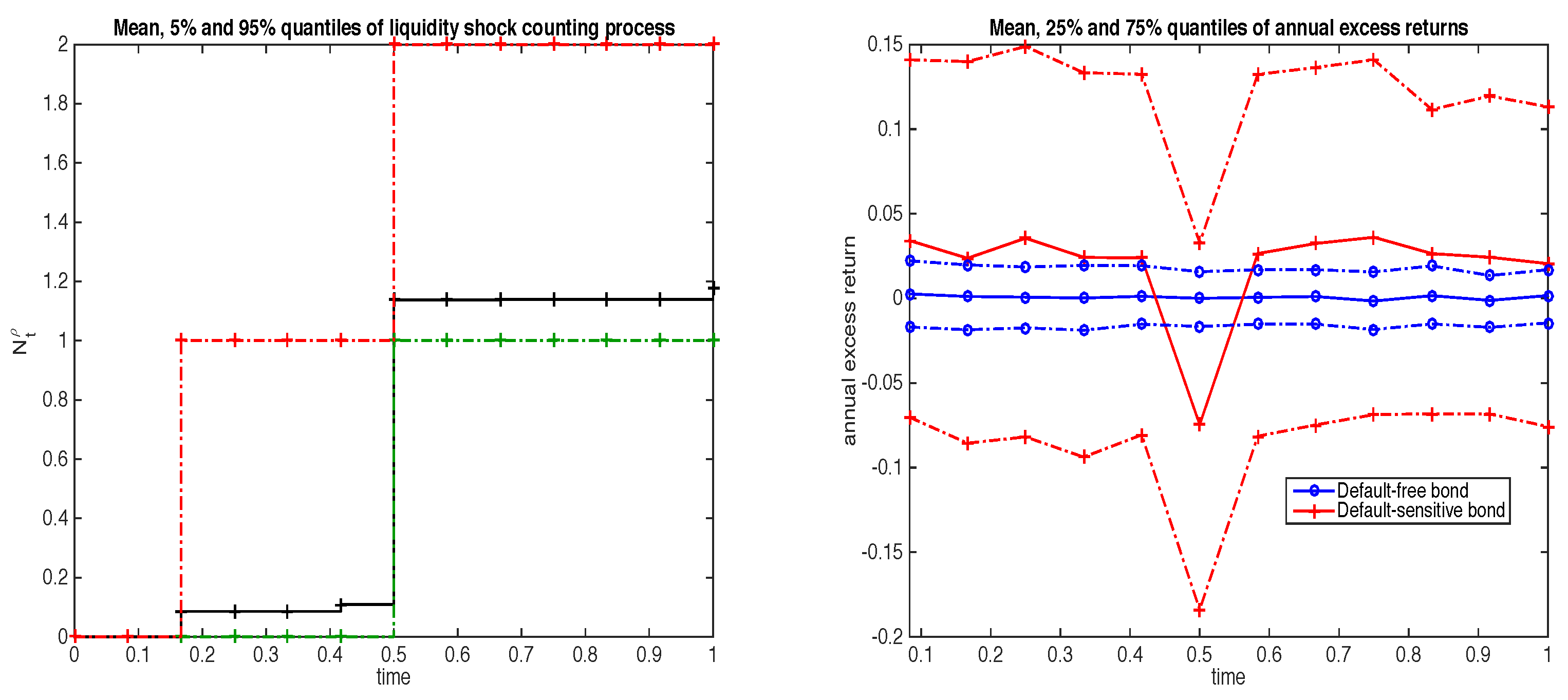
Concerning the liquidity risk, the parameters are chosen such that the average number of liquidity shocks per year is between 1 and 2 (see Figure 1). In addition, we assume for the numerical simulation that the illiquidity impact is given by
where is a positive parameter that represents the sensitivity of the shock severity with respect to the number of liquidity shocks. The greater the number of shocks is in the period, the greater the negative impact is on the returns of the default-sensitive bond. Then, is chosen such that , i.e., given a liquidity shock, the expected impact on the annual return rate is . The interest rate and default intensity processes are supposed to follow an independent CIR process. The interest rates are calibrated on the 10-year ZC swap and the default intensity on the credit spread of the 10-year Italian government bonds on year 2016 with a monthly frequency. We choose to calibrate the data for year 2016 because it was a hectic year during which the risk premia increased substantially, especially following the vote in favor of Brexit. This setting is called the central model specification.
Figure 1.
Empirical mean: 25% and 75% quantiles of sampled paths of (left) and of sampled paths of the risky assets’ annual excess return rates and (right) at the end of each rebalancing period, i.e., at time .
In the central model, we additionally consider some linear constraints on optimal proportions, which correspond to the SAA provided by the asset owner to the asset manager. The optimal proportions on risky assets are such that the sum is between 0 and ; the proportion of risk-free assets is less than , i.e., ; and each component is between 0 and . These conditions translate into a linear system of inequality constraints of the form , where
and
The optimization problem (27) corresponds to a Markov decision process with an underlying Markovian state process defined as with
It is worth noting that the liquidity shock counting process is not a state variable since it only appears through its independent increments. The Markovian state process has the following approximated discrete time dynamics3:
where and are two independent sequences of i.i.d. standard Gaussian random variables. To facilitate comparisons in the solutions of (27), we assume that the Poisson noises in the doubly stochastic Poisson processes and N are frozen to a deterministic path.4
We consider the methodology introduced by Brandt et al. (2005) to find numerical solutions of the optimization problem (27). We first derive the Bellman equation associated with the considered Markov decision process. The cost-to-go function and corresponding optimal strategies can then be obtained at each rebalancing date using a backward iterative procedure (dynamic programming). At each iteration date, we perform a Taylor expansion of the cost-to-go function, which gives an approximation of optimal strategies as solutions of a quadratic optimization problem. The coefficients of this quadratic optimization problem are expressed in the form of conditional expectations, which are estimated by simulation-regression techniques (least square Monte Carlo) and using previously computed strategies. The numerical procedure is described in Appendix B.
Figure 1 (left side) shows that most sample paths of exhibit a single liquidity shock at the sixth period ().5 As a consequence, the excess return rate on the default-sensitive bond falls by about 10% in this period (Figure 1, right side).
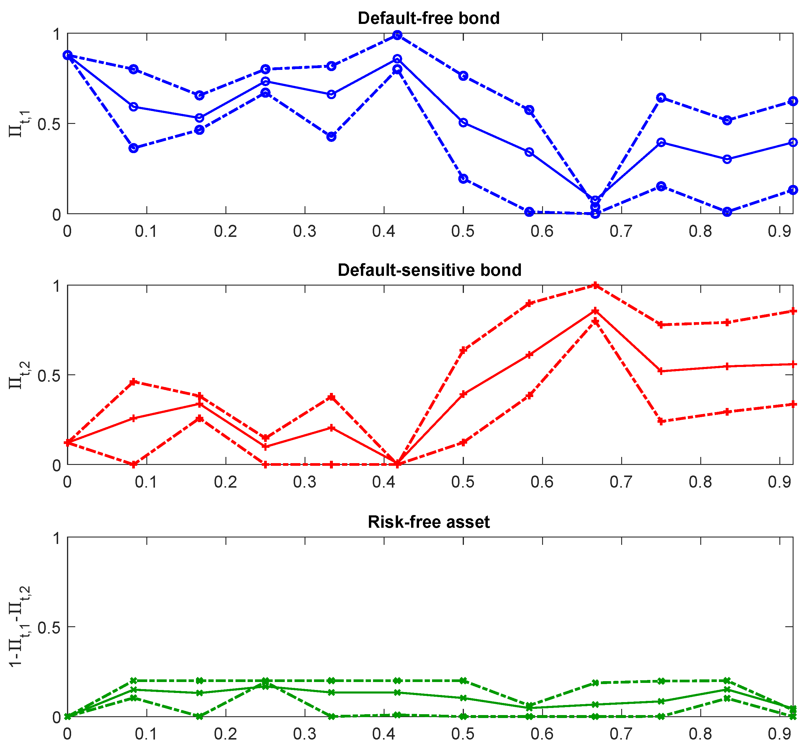
Figure 2 displays the optimal proportions of the default-free bond, the default-sensitive bond, and the risk-free assets obtained as the solution of (27). As required by the allocation constraints, the proportion of the risk-free asset is always smaller than 20%. In addition, the trend of optimal strategies is strongly affected by the occurrence of the liquidity shock at the sixth period (see Figure 1, right side, and Figure 2). The proportion invested in the default-sensitive bond whose return falls by 10% due to liquidity shock at the sixth period goes to zero just before the shock and is smaller than the proportion in the default-free bond before the shock6. After the shock, the proportion of the default-sensitive bond increases, which allows for a higher return of the asset portfolio.
Figure 2.
Empirical mean: 25% and 75% quantiles of the optimal proportions invested in the default-free bond (up), default-sensitive bond (middle), and risk-free asset (bottom).
We analyze the performance of the obtained optimal strategies when the latter are applied to sampled paths of the state process.7 Figure 3 compares the optimal penalized utilities of wealth (upper left side), asset values (upper right side), and asset-liability ratios (bottom) at each date with the corresponding values obtained when (i) using the risk-free asset only (referred to as the “risk-free strategy”) and (ii) when proportions in the three assets are fixed to a constant value over time (10% in the risk-free asset, 40% in the default-free bond, and 50% in the default-sensitive bond, referred to as the “fixed-proportion strategy”). We observe that the optimal strategy, on average, outperforms the fixed-proportion and risk-free strategies, and exhibits lower variability than the fixed-proportion strategy. The negative trend in asset portfolio values is due to the surrender payments in each period, i.e., the positive term in (26).
Figure 3.
Empirical mean: 25% and 75 % quantiles of the penalized utilities of wealth (upper left), asset values (upper right), and asset-liability ratios (bottom) when using the risk-free asset only, when using fixed proportions invested in the three considered assets (10% in the risk-free asset, 40% in the default-free bond, and 50% in the default-sensitive bond), and when using the optimal proportions in the three assets as solution of (27).
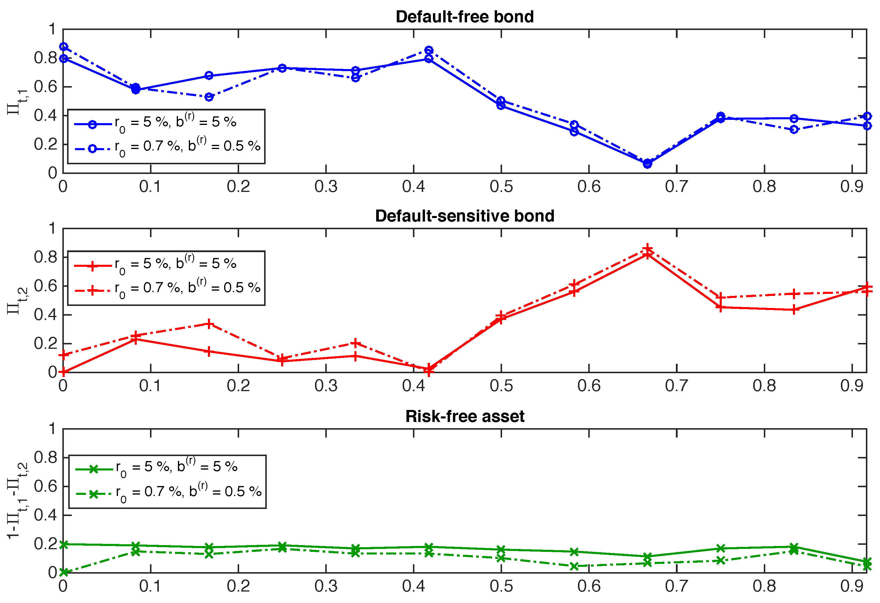
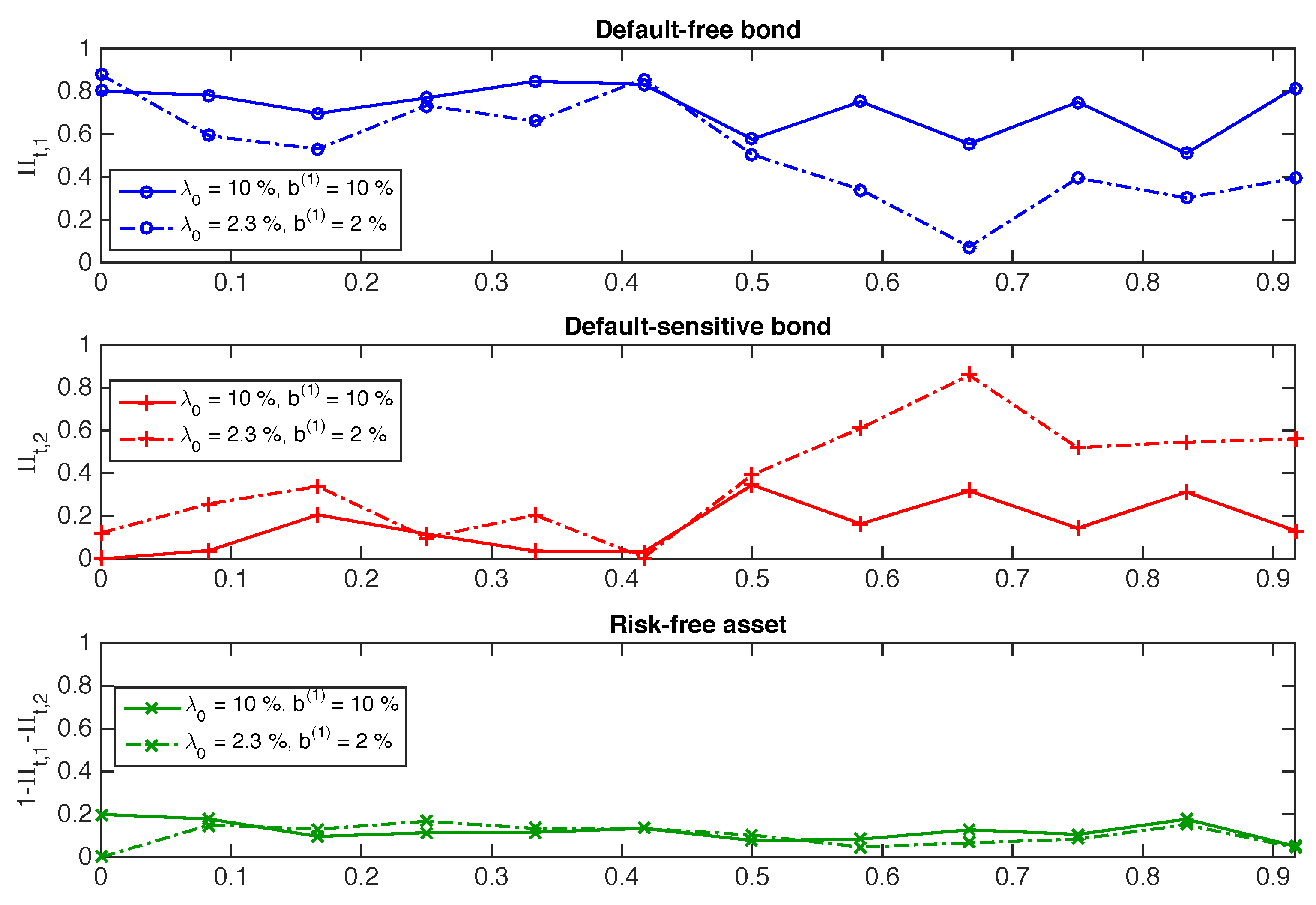
We now study how optimal strategies are impacted by a change in input parameters. Figure 4 compares the optimal strategy in the central model specification and when the level of the short-rate process increases from 0.7% to 5%. This has two direct consequences. First, the annual return on the risk-free asset increases with the same magnitude level. Second, the average annual surrender rate doubles and goes from 10% to 20%. Figure 4 shows that the optimal proportion in the risk-free asset increases to nearly , which is its maximum possible value. The optimal proportion invested in the default-sensitive bond slightly decreases over the period.
Figure 4.
Sensitivity of optimal strategies to a change in the level of short rate.
Figure 5 compares the optimal strategy in the central model specification and when the level of the default intensity process increases from 2.3% to 10%. This change negatively impacts the price of the default-sensitive bond, which increases the long-term return of this bond; however, it triples the frequency of withdrawal payments and multiples the frequency of liquidity shocks by eight. Therefore, the main effect is a significant fall of the optimal proportions invested in the default-sensitive bond to reduce the risk of losses arising from the forced sales of assets to meet redemptions.
Figure 5.
Sensitivity of optimal strategies to a change in the level of default intensity.
These results show how accounting for joint liquidity risks (on the asset side) and withdrawal risks (on the liability side; i) substantially modifies the optimal allocation of a financial institution offering guaranteed-capital contracts to mitigate its default risk and (ii) improves both its solvency ratio and asset returns.
Appendix C provides an additional sensitivity analysis with respect to change in , , , and .
4. Conclusions
This study examined an optimal investment allocation problem for a financial institution offering capital-guaranteed contracts that incorporate the option of withdrawal at any time. Both the financial assets and the withdrawal frequency are influenced by market factors including credit quality, liquidity risk, and interest rate level. By using a dynamic programming approach, we provide a recursive formula for obtaining the optimal strategy for this utility maximization problem under several asset-liability constraints. The numerical resolution provides a detailed description of the optimal trading strategies.
This paper contributes to the existing literature (e.g., Berry-Stölzle 2008) by highlighting the importance, for an institutional asset manager, of taking into account the snowball effect that may occur in certain market configurations, such as financial crises. Indeed, the combination of redemptions on the liabilities side and financial illiquidity on the assets side can lead to insolvency for the financial institution.
We show that financial institutions should adjust their optimal asset allocation to account for the illiquidity mismatch between assets and liabilities. Specifically, to mitigate its default risk, a financial institution needs to reduce its exposure to risky assets when it expects a rise in credit risk (i.e., during financial turmoil) that can trigger a decrease in the liquidity of assets and an increase in redemptions, thereby forcing the institution to sell assets at discounted prices and deteriorate its solvency.
The method used in this paper has some limitations, however. First, we modeled the transaction dates as discrete. Although this assumption is generally quite realistic, it is possible that the frequency of transactions may be higher during certain periods, e.g., during times of crisis. A possible amendment to the model would be to consider transaction dates based on stopping times. Besides, we fixed the horizon T of the problem. The model could be reconstructed by considering a horizon based on a stopping time, for example, when the solvency ratio crosses a certain threshold. Finally, in the numerical simulations, we set the shock time. It would be interesting to analyze the optimal allocation when the shock time is an inaccessible stopping time, i.e., during which we do not observe the effect of the reduction of the allocation before the shock.
Building on this work, several avenues of research may be considered. First, can we establish a link between the risk aversion and parameters , , and in the constraints of the problem? Moreover, from the point of view of prudential regulation, how should parameters , , and be calibrated? Second, liquidity stresses may materialize differently, for example, without any major impact on the selling price but simply as a limited supply of assets. What would happen to the optimal allocation in this case? Third, we built our model on a run-off portfolio where the terms of the contracts may be very different from the new market conditions. The institution that continues to offer new contracts modifies its solvency and capacity to withstand financial shocks. What would happen to the optimal allocation when we take into account the arrival of new business? Fourth, replicating a numerical analysis with a large number of assets with different correlations can offer richer solutions to financial institutions. On a theoretical level, the same model can be enriched by developing the dynamics of liabilities. Finally, the risk analysis of liquidity mismatch between assets and liabilities can be extended to the case of exchange-traded funds that offer liquidity to clients, which is often better than the liquidity of the assets in which they invest.
Author Contributions
Conceptualization, A.C., Y.J., C.Y.R. and O.D.Z.; methodology, A.C., Y.J., C.Y.R. and O.D.Z.; software, A.C., Y.J., C.Y.R. and O.D.Z.; validation, A.C., Y.J., C.Y.R. and O.D.Z.; formal analysis, A.C., Y.J., C.Y.R. and O.D.Z.; investigation, A.C., Y.J., C.Y.R. and O.D.Z.; resources, A.C., Y.J., C.Y.R. and O.D.Z.; data curation, A.C., Y.J., C.Y.R. and O.D.Z.; writing—original draft preparation, A.C., Y.J., C.Y.R. and O.D.Z.; writing—review and editing, A.C., Y.J., C.Y.R. and O.D.Z.; visualization, A.C., Y.J., C.Y.R. and O.D.Z.; supervision, A.C., Y.J., C.Y.R. and O.D.Z.; project administration, A.C., Y.J., C.Y.R. and O.D.Z.; funding acquisition, A.C., Y.J., C.Y.R. and O.D.Z. All authors have read and agreed to the published version of the manuscript.
Funding
This work was funded by Groupama Asset Management.
Data Availability Statement
The data and code are available from the authors.
Acknowledgments
The working paper reflects the opinions of the authors and do not necessarily express the views of Groupama Asset Management. This work has also benefited from partial support from Institut Europlace de Finance.
Conflicts of Interest
The authors declare no conflict of interest.
Appendix A. Stochastic Dynamics of Financial Assets
For the numerical illustrations, we consider that the asset manager can invest in three assets (): the risk-free asset (the deposit account with a stochastic instantaneous return rate), a default-free zero-coupon bond with maturity , and a default-sensitive zero-coupon bond with maturity .
We begin with a “default-free” zero-coupon bond, which only bears the interest rate evolution and adopts the affine term structure modeling approach for the bond pricing. We assume that, under the risk-neutral probability measure , the short-term interest rate r is described by a mean-reverting affine diffusion of the form
where is a Brownian motion under the risk-neutral probability ; a and b are positive parameters; and is a positive deterministic function. The price of the cash is given by
The price of the default-free zero-coupon bond of maturity is given by
Given the affine structure of the model (cf. Duffie 2005), the zero-coupon bond price can be expressed as
where and are deterministic functions that can be expressed in the closed form, e.g., in the Vasicek or CIR models. The risk-neutral dynamics of the zero-coupon price is then given by
where . By the Girsanov theorem, an -adapted process exists such that, under the historical probability , the dynamics of can be expressed as
The change of the probability measure is defined by the Radon–Nikodym derivative
In the following section, we consider the specific case of the CIR model, i.e., when . Moreover, if we require that the dynamics of r remain in the same family after the equivalent change of the probability measure, the suitable choice of the interest-rate risk premium is such that
The risk-neutral parameters in (A1) are then such that , , and the functions and of the arbitrage-free price of the zero-coupon bond with maturity in (A4) are given by
Then, we consider a defaultable bond and explain how it is evaluated. The endogenous credit risk is characterized by an individual default intensity. More precisely, we assume that the credit risk of the risky bond is characterized by the default intensity process , which is an -adapted process. In addition, we assume that belongs to the same class of affine processes as the short-term interest rate such that the term structure of the defaultable bond can be represented in the same way, that is
where are constants, is of the same type as the volatility function of (A1), and is a Brownian motion independent of under . Hence, the pre-default price of the bond with maturity at time is given by
Then, by using Duffie (2005), the risky bond price can be expressed as
where and are as in (A4) and both and are deterministic functions such that
Moreover, one has
where . We consider the following change of the probability measure
Using this change of the probability measure,
with , . The pre-default dynamic of the bond under the historical probability is given by
while the dynamics of the bond given in (A6) under the historical probability is unchanged.
Appendix B
Appendix B.1. Value Function and Bellman Equation
Without loss of generality, let us consider the time grid instead of . For , we define the value function J as
The Bellman equation is given by
where
Given (26), the time value function writes
where we define .
Moreover, let
A Taylor expansion of around is given by
At each time t, we want to find , which maximizes under the linear inequality constraint . Let us define
An approximation of the optimal strategy can be obtained as the solution of the following quadratic optimization problem.
Note that without the inequality constraint, the solution is explicit and given by
In the presence of linear inequality constraints, we rely on a quadratic programming solver.
Appendix B.2. Computation of and
Let us recall that
or equivalently
with
where is the deterministic function such that . Note that
Using the prescribed (26) dynamics of X, we can write the terminal asset portfolio value in the following way:
Let us define
where are the optimal portfolio weights at the rebalancing date . Thus, we can write
It follows that
Additionally, it follows that
and
Note that
where
Then, assuming that optimal strategies have been computed at time for different sample paths of , we can estimate and by regression of and on explanatory variables .
Appendix B.3. Numerical Procedure
The Bellman equations are solved using a forward–backward iterative procedure on the time grid . The first forward procedure aims at constructing a suitable discrete representation of the state space. The second backward procedure corresponds to solving Bellman’s equation on this discretized state space. Once optimal strategies have been pre-computed, their performances are assessed on sample paths of the exogenous state variables.
- Discretizing the state space by simulating state processes. We generate n independent sample paths of the exogenous state processes r and (and accordingly modify paths of N) on the time grid . At each time t, the state space grid is been defined as the collection of sample values taken by these processes. Knowing that optimal strategies are constrained in a bounded domain, the state space for the state variable X is approximated by collecting, at each time , sample values of X generated from (26) using sampled paths of r and , and by employing, at each rebalancing date, uniformly distributed sampled strategies on the bounded domain.
- Solving the Bellman equation on the discretized state space
- The time-T value of cost-to-go function is initialized on each point of the time-T state space grid using (A16).
- For each time iteration t, and for any point in the time-t state space grid, is obtained as the solution of (A17). The coefficients of the quadratic optimization problems and are approximated using previously computed values of interpolated on the corresponding state space grid and using regression on the sample path of Z.
- Assessing the performance of optimal strategies. For each sample path of the state processes r and , we compute the value of the optimal asset portfolio by using, at each rebalancing date, the optimal strategy that best represents the state variable current value. The employed strategy is found by interpolating pre-computed optimal strategies on the current state space grid. Based on these sample paths, we can then compute sample paths of the optimal asset portfolio together with any relevant statistics.
Appendix C. Other Sensitivity Analyses
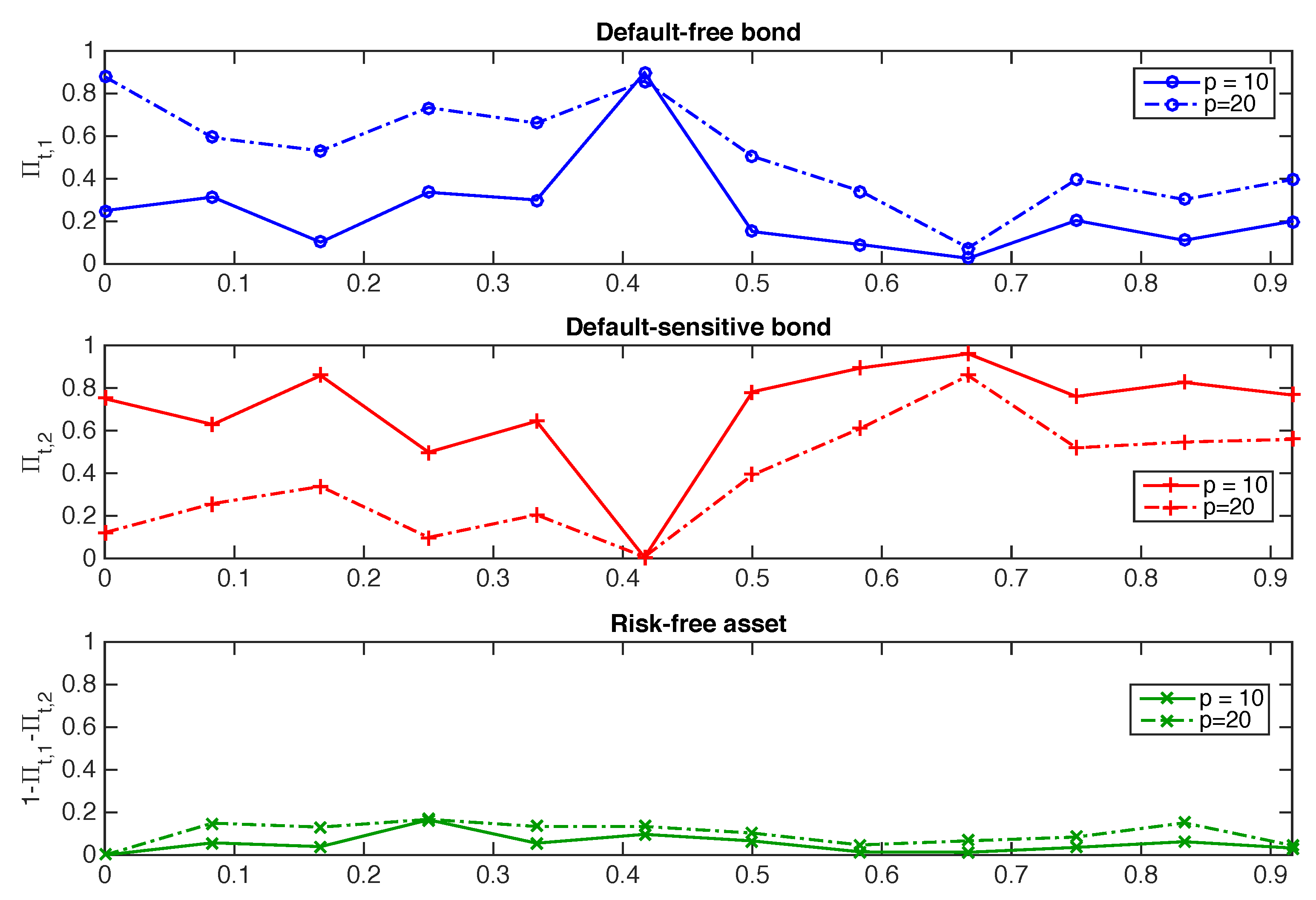
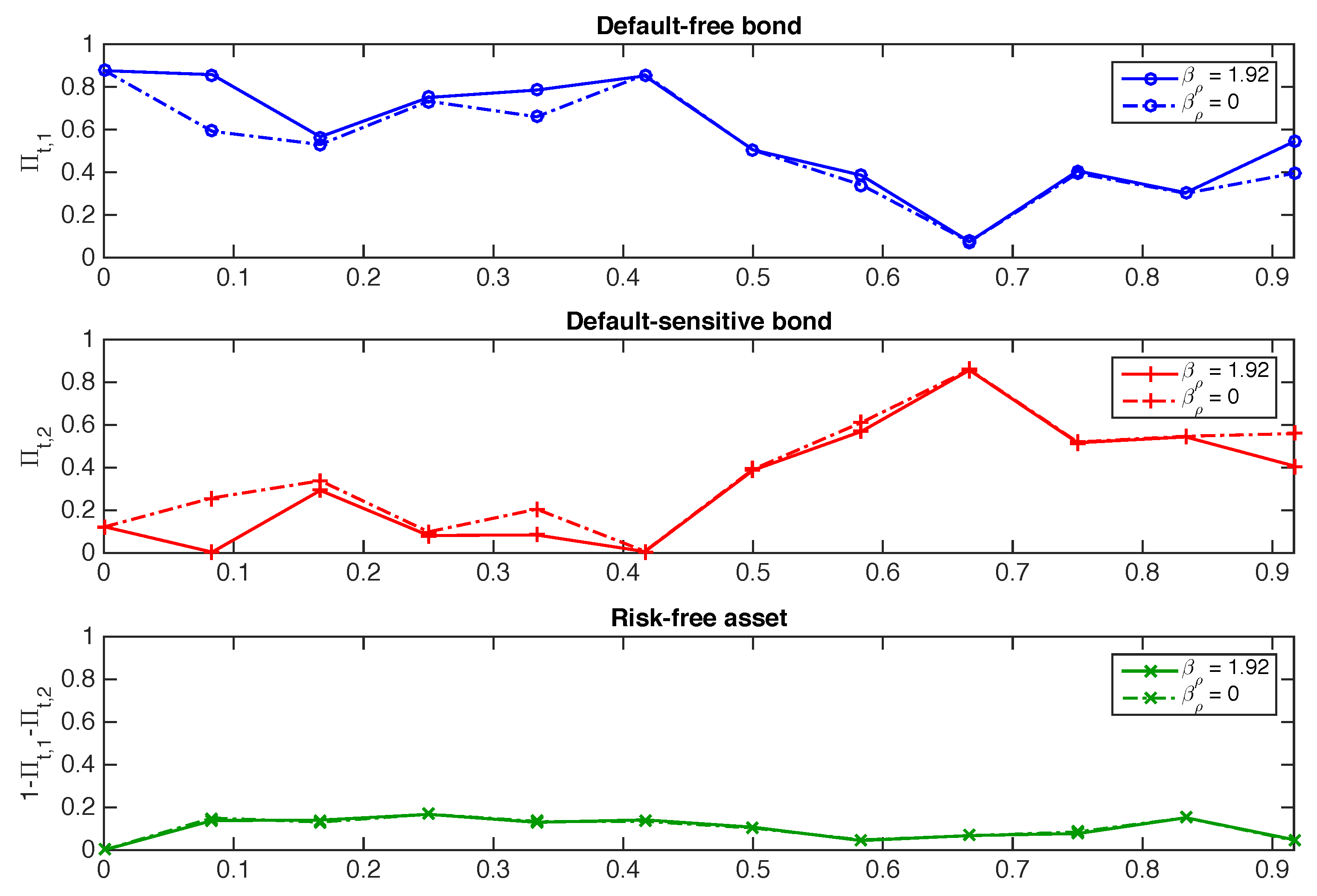
Figure A1 compares the optimal strategy in the central model specification and when the degree of risk aversion decreases from to . Consistently, we observe that the optimal proportions in the default-sensitive bond (the riskiest asset) uniformly increase over the period and the proportions of the two other assets uniformly decrease over the period.
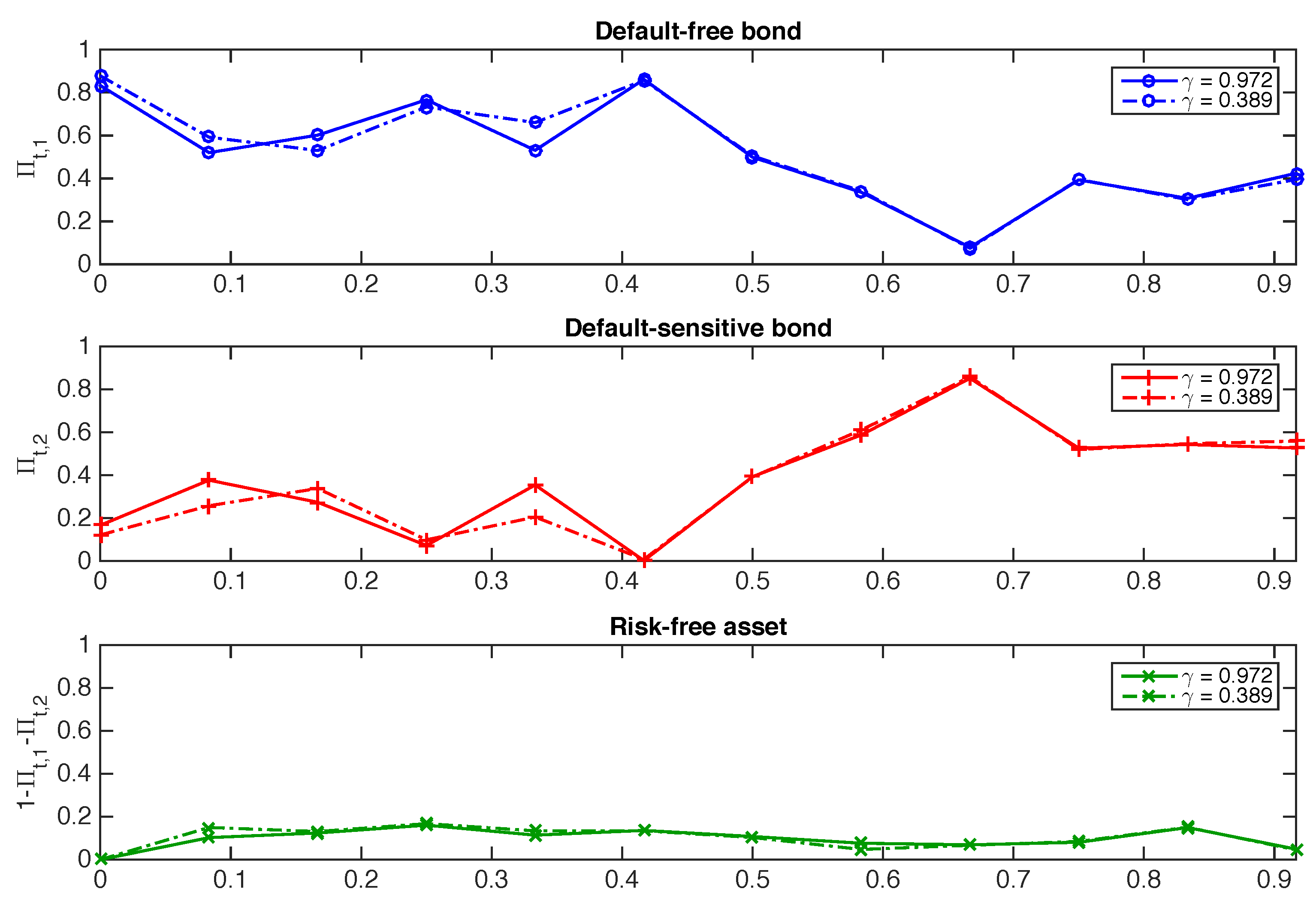
Sensitivities of the optimal strategies to a change in , , , and are depicted in Figure A2, Figure A3, Figure A4 and Figure A5, respectively. When parameter increases, the number of liquidity shocks over increases; therefore, we observe a reduction of the proportion invested in the defaultable bond. When parameter increases, the solvency penalty is stronger and, as a result, the proportion invested in the riskier asset (the more volatile one) decreases.
Figure A1.
Sensitivity of optimal strategies to a change in the degree of risk aversion.
Figure A2.
Sensitivity of optimal strategies to a change in .
Figure A3.
Sensitivity of optimal strategies to a change in .
Figure A4.
Sensitivity of optimal strategies to a change in .
Figure A5.
Sensitivity of optimal strategies to a change in .
Notes
| 1 | The investment portfolio value may become negative if almost all customers decide to withdraw money from their contract and if the value of the invested assets falls, but this happens with a very low probability (see, e.g., the case study considered in Section 3 and Figure 3). |
| 2 | See Section 2.3 for a more detailed discussion. |
| 3 | Note that the discrete versions of the CIR processes have been simulated using the methodology proposed in Alfonsi (2005). |
| 4 | Meaning that when simulating these Cox processes from a standard Poisson process, only one single deterministic path of the Poisson process is used. |
| 5 | Even if Poisson noise is frozen to a deterministic path, the differences in sampled paths is due to its stochastic intensity . |
| 6 | The intensity of the liquidity shock is observed just before the jump and therefore the optimal allocation takes it into account. |
| 7 | We used the same to numerically solve Bellman equations. |
References
- Alfonsi, Aurelien. 2005. On the discretization schemes for the CIR (and Bessel squared) processes. Monte Carlo Methods and Applications 11. [Google Scholar] [CrossRef]
- Allen, Franklin, and Douglas Gale. 2004. Financial Intermediaries and Markets. Econometrica 72: 1023–61. [Google Scholar] [CrossRef] [Green Version]
- Bao, Jack, Jun Pan, and Jiang Wang. 2011. The Illiquidity of Corporate Bonds. The Journal of Finance 66: 911–46. [Google Scholar] [CrossRef] [Green Version]
- Berry-Stölzle, Thomas R. 2008. The impact of illiquidity on the asset management of insurance companies. Insurance: Mathematics and Economics 43: 1–14. [Google Scholar] [CrossRef]
- Blanchard, Romain, and Laurence Carassus. 2018. Multiple-priors optimal investment in discrete time for unbounded utility function. The Annals of Applied Probability 28: 1856–92. [Google Scholar] [CrossRef] [Green Version]
- Boyle, Phelim, and Weidong Tian. 2007. Portfolio management with constraints. Mathematical Finance 17: 319–43. [Google Scholar] [CrossRef]
- Brandt, Michael W., Amit Goyal, Pedro Santa-Clara, and Jonathan R. Stroud. 2005. A Simulation Approach to Dynamic Portfolio Choice with an Application to Learning About Return Predictability. Review of Financial Studies 18: 831–73. [Google Scholar] [CrossRef] [Green Version]
- Brunnermeier, Markus K., and Lasse Heje Pedersen. 2008. Market Liquidity and Funding Liquidity. Review of Financial Studies 22: 2201–38. [Google Scholar] [CrossRef] [Green Version]
- Cao, Charles, and Lubomir Petrasek. 2014. Liquidity risk in stock returns: An event-study perspective. Journal of Banking & Finance 45: 72–83. [Google Scholar] [CrossRef]
- Carr, Peter, and Vadim Linetsky. 2006. A jump to default extended CEV model: An application of Bessel processes. Finance and Stochastics 10: 303–30. [Google Scholar] [CrossRef]
- Chen, Hui, Rui Cui, Zhiguo He, and Konstantin Milbradt. 2017. Quantifying Liquidity and Default Risks of Corporate Bonds over the Business Cycle. The Review of Financial Studies 31: 852–97. [Google Scholar] [CrossRef]
- Chen, Tsung-Kang, Hsien-Hsing Liao, and Pei-Ling Tsai. 2011. Internal liquidity risk in corporate bond yield spreads. Journal of Banking & Finance 35: 978–87. [Google Scholar] [CrossRef]
- Cousin, Areski, Ying Jiao, Christian Y. Robert, and Olivier David Zerbib. 2016. Asset allocation strategies in the presence of liability constraints. Insurance: Mathematics and Economics 70: 327–38. [Google Scholar] [CrossRef]
- Dick-Nielsen, Jens, Peter Feldhütter, and David Lando. 2012. Corporate bond liquidity before and after the onset of the subprime crisis. Journal of Financial Economics 103: 471–92. [Google Scholar] [CrossRef] [Green Version]
- Duffie, Darrell. 2005. Credit risk modeling with affine processes. Journal of Banking & Finance 29: 2751–802. [Google Scholar] [CrossRef]
- El Karoui, Nicole. 1981. Les aspects probabilistes du contrôle stochastique. In Ninth Saint Flour Probability Summer School—1979 (Saint Flour, 1979). Lecture Notes in Math. Berlin and New York: Springer, vol. 876, pp. 73–238. [Google Scholar]
- El Karoui, Nicole, Monique Jeanblanc, and Vincent Lacoste. 2005. Optimal portfolio management with American capital guarantee. Journal of Economic Dynamics and Control 29: 449–68. [Google Scholar] [CrossRef]
- Ericsson, Jan, and Olivier Renault. 2006. Liquidity and Credit Risk. The Journal of Finance 61: 2219–50. [Google Scholar] [CrossRef]
- Favero, Carlo, Marco Pagano, and Ernst-Ludwig von Thadden. 2009. How Does Liquidity Affect Government Bond Yields? Journal of Financial and Quantitative Analysis 45: 107–34. [Google Scholar] [CrossRef] [Green Version]
- Feng, Runhuan, and Jan Vecer. 2016. Risk based capital for guaranteed minimum withdrawal benefit. Quantitative Finance 17: 471–78. [Google Scholar] [CrossRef]
- Föllmer, Hans, and Peter Leukert. 1999. Quantile hedging. Finance and Stochastics 3: 251–73. [Google Scholar] [CrossRef]
- Föllmer, Hans, and Peter Leukert. 2000. Efficient hedging: Cost vs. shortfall risk. Finance and Stochastics 4: 117–46. [Google Scholar]
- Frauendorfer, Karl, and Michael Schürle. 2003. Management of non-maturing deposits by multistage stochastic programming. European Journal of Operational Research 151: 602–16. [Google Scholar] [CrossRef] [Green Version]
- Goyenko, Ruslan, Avanidhar Subrahmanyam, and Andrey Ukhov. 2010. The Term Structure of Bond Market Liquidity and Its Implications for Expected Bond Returns. Journal of Financial and Quantitative Analysis 46: 111–39. [Google Scholar] [CrossRef] [Green Version]
- Goyenko, Ruslan Y., and Andrey D. Ukhov. 2009. Stock and Bond Market Liquidity: A Long-Run Empirical Analysis. Journal of Financial and Quantitative Analysis 44: 189–212. [Google Scholar] [CrossRef] [Green Version]
- Gundel, Anne, and Stefan Weber. 2007. Robust utility maximization with limited downside risk in incomplete markets. Stochastic Processes and Their Applications 117: 1663–88. [Google Scholar] [CrossRef] [Green Version]
- Jiao, Ying, Olivier Klopfenstein, and Peter Tankov. 2017. Hedging under multiple risk constraints. Finance and Stochastics 21: 361–96. [Google Scholar] [CrossRef] [Green Version]
- Kalkbrener, Michael, and Jan Willing. 2004. Risk management of non-maturing liabilities. Journal of Banking & Finance 28: 1547–68. [Google Scholar] [CrossRef]
- Kling, Alexander, Frederik Ruez, and Jochen Russ. 2013. The Impact of stochastic volatility on pricing, hedging, and hedge efficiency of withdrawal benefit guarantees in variable annuities. ASTIN Bulletin 41: 511–45. [Google Scholar] [CrossRef]
- Lin, X. Sheldon, and Shuai Yang. 2020. Fast and efficient nested simulation for large variable annuity portfolios: A surrogate modeling approach. Insurance: Mathematics and Economics 91: 85–103. [Google Scholar] [CrossRef]
- Nyström, Kaj. 2008. On deposit volumes and the valuation of non-maturing liabilities. Journal of Economic Dynamics and Control 32: 709–56. [Google Scholar] [CrossRef]
- Pan, Jian, and Qingxian Xiao. 2017. Optimal asset–liability management with liquidity constraints and stochastic interest rates in the expected utility framework. Journal of Computational and Applied Mathematics 317: 371–87. [Google Scholar] [CrossRef]
- Pham, Huyên. 2009. Continuous-time stochastic control and optimization with financial applications. In Stochastic Modelling and Applied Probability. Berlin: Springer, vol. 61, pp. xviii, 232. [Google Scholar] [CrossRef]
- Shevchenko, Pavel V., and Xiaolin Luo. 2017. Valuation of variable annuities with Guaranteed Minimum Withdrawal Benefit under stochastic interest rate. Insurance: Mathematics and Economics 76: 104–17. [Google Scholar] [CrossRef] [Green Version]
- Steinorth, Petra, and Olivia S. Mitchell. 2015. Valuing variable annuities with guaranteed minimum lifetime withdrawal benefits. Insurance: Mathematics and Economics 64: 246–58. [Google Scholar] [CrossRef] [Green Version]
- Wang, Jindong, and Wei Xu. 2020. Risk based capital for variable annuity under stochastic interest rate. ASTIN Bulletin 50: 959–99. [Google Scholar] [CrossRef]
Publisher’s Note: MDPI stays neutral with regard to jurisdictional claims in published maps and institutional affiliations. |
© 2022 by the authors. Licensee MDPI, Basel, Switzerland. This article is an open access article distributed under the terms and conditions of the Creative Commons Attribution (CC BY) license (https://creativecommons.org/licenses/by/4.0/).