New Definition of Default—Recalibration of Credit Risk Models Using Bayesian Approach

Abstract

After the financial crisis, the European Banking Authority (EBA) has established tighter standards around the definition of default (Capital Requirements Regulation CRR Article 178, EBA/GL/2017/16) to increase the degree of comparability and consistency in credit risk measurement and capital frameworks across banks and financial institutions. Requirements of the new definition of default (DoD) concern how banks recognize credit defaults for prudential purposes and include quantitative impact analysis and new rules of materiality. In this approach, the number and timing of defaults affect the validity of currently used risk models and processes. The recommendation presented in this paper is to address current gaps by considering a Bayesian approach for PD recalibration based on insights derived from both simulated and empirical data (e.g., a priori and a posteriori distributions). A Bayesian approach was used in two steps: to calculate the Long Run Average (LRA) on both simulated and empirical data and for the final model calibration to the posterior LRA. The Bayesian approach result for the PD LRA was slightly lower than the one calculated based on classical logistic regression. It also decreased for the historically observed LRA that included the most recent empirical data. The Bayesian methodology was used to make the LRA more objective, but it also helps to better align the LRA not only with the empirical data but also with the most recent ones.

1. Introduction

Following the financial crisis, EBA has established tighter standards around the definition of default (Capital Requirements Regulation—CRR Article 178, EBA/GL/2017/16) (EBA 2017) to achieve a higher comparability and consistency in models used for credit risk measurement and procedures and capital frameworks across banks and financial institutions. These requirements were supposed to be implemented by the end of 2020.

The initial deadline for the implementation (for all banks using IRB approach) was the 1st of January 2021. These deadlines were under discussion with European Central Bank (ECB) by many banks, and now they are under further revision by ECB due to COVID—19 circumstances (EBA 2016b).

Banks were allowed to choose either a one-step, or a two-step approach:

• One-step approach—the introduction of the new definition of default (DoD) and recalibration of all relevant models in one step;
• Two-step approach—first the introduction of the new DoD and then recalibration of relevant models.

The two-step approach was introduced because ECB realized that one-step approach would most likely automatically trigger a material change of all models within a bank.

The new DoD concern how banks recognize credit defaults for prudential purposes and also include quantitative impact analysis and new rules of materiality. In this approach, the number and timing of defaults determine whether existing models and processes are valid. Banks need to update their risk management practices and support pricing and accounting decisions related not only to the expected credit loss methodology (according to International Financial Reporting Standards—IFRS 9) (EU 2016) but also those related to capital requirements models (according to Internal Ratings Based Approach -IRB and Internal Capital Adequacy Assessment Process—ICAAP) (ICAAP 2018).

These extensive and very detailed guidelines often challenge information technology (IT) infrastructure, processes, data engines and data analytics, commonly used model risk platforms, model implementation and execution and automated solutions (BCBS 2013). In addition, these new standards have a significant impact on risk governance and management, frameworks and methodologies, data quality process assessments and reviews, as well as model recalibration needs and internal management policies and approval processes (Basel 2010, 2014).

In recent research on the credit risk parameters modeling, different approaches incorporate small samples problem incorporation (Zięba 2017), unbalanced samples or unresolved cases for LGD. Different techniques are proposed starting with traditional logistic or linear regression approach, two-stage modeling, ensemble models (Papouskova and Hajek 2019), and new machine learning methods or non-parametric approach (Peláez Suárez et al. 2021). In the literature of the PD modeling mostly a frequentist approach is applied (Bellotti and Crook 2009; Crone and Finlay 2012; Lessmann et al. 2015; Wang et al. 2020), while only limited use of a Bayesian approach is present (Bijak and Matuszyk 2017; Bijak and Thomas 2015). Among the papers using a Bayesian approach, many use non-informative priors on the assumption of the likelihood normally asymptotically distributed with large data (Bijak and Thomas 2015). Some papers emphasize the importance of expert information and use that to gain informative priors (Jacobs and Kiefer 2010; Kiefer 2009) or use coefficient estimates of past data as priors for current data (Bijak and Matuszyk 2017). However, we find that effective use of informative priors is still a gap to be covered.

The main contribution of this paper is to propose an approach to complement the scarce observational data post redefinition of DoD with simulated data. The Bayesian method was applied to anticipate this simulated and empirical data for a basic credit risk measure: probability of default (PD) re-calibration. Such example of Bayesian approach utilization in modeling and calibration of credit risk parameters is promising for trying to incorporate such approach in calibration of PD, using parameters estimated on empirical data for new DoD as prior information. For other parameters such as loss given default (LGD) and exposure of default (EAD) only a theoretical approach was proposed.

The paper is organized as follows: Section 1 provides an overview of the main implications of regulatory requirements impacting banks from a risk management perspective, with a focus on credit risk models. In this section a literature review focused on Bayesian approach is presented. Section 2 describes current challenges from a modeling perspective and discusses a methodological proposal to address these gaps. Section 3 provides an empirical example of application on real data for retail customers. Final section contains concluding remarks and suggestions for future research.

2. Implications of the New Definition of Default—Literature Review

This section provides a summary of the main changes implied by the new DoD and its impacts for credit risk modeling with specific emphasis for the institution under study in this article (one of European commercial banks). The literature review is limited to regulatory background and to Bayesian approach in research as the main focus of the paper.

The regulation contains specific requirements addressing specific event identification and threshold calculations. As a high-level overview, the main directions of the introduced changes can be split into specific focus areas: Days Past Due (DpD) calculation, Unlikeliness to Pay Criteria (UTP), Return to Non-Default Status (probation period), and Other Significant Changes (EBA/GL/2017/16, EBA/RTS/2016/06) (EBA 2014, 2016a, 2016b, 2017, 2020).

Materiality thresholds for days past due (DpD) includes not only absolute but also relative materiality thresholds for counting DpD until the event of default at 90 DpD (for retail exposures: 1% relative and 100 euros absolute, for non-retail exposures: 1% relative and 500 euros absolute).

The amounts past due represent the sum of all amounts past due, including all fees, interests, and principal. For the relative threshold calculation, this amount is divided by the total on-balance and off-balance exposure. If the principal is not repaid when an interest only loan expires, counting DpD starts from that date despite the fact that the obligor continues to pay interest.

Unlikeness to pay criteria (UTPs) will be recognized if the credit obligation gets a non-accrued status according to the accounting framework. Specific credit risk adjustments (SCRA) can be as follows: (i) sale of client’s credit obligation recognized as defaulted if economic loss exceeds 5%, (ii) distressed restructuring if the net present value of the obligation decreases by more than 1% the obligation is considered defaulted, (iii) bankruptcy, (iv) additional indications of UTP (including fraud, significant increase in obligor leverage, individual voluntary arrangements, significant delays in payment to other creditors, impaired credit history indicators, expecting worst status).

A minimum probation period of three months is required for all defaults. The exemption stands for distressed restructurings where applies a 1-year minimum probation period. It is required to monitor the effectiveness of the cure policy on a regular basis, including also impact on cure rates and impact on multiple defaults.

Indeed, to implement the new DoD it is important to consider the holistic view of all processes impacted. In this respect, the key aspect to consider is a robust control framework from a risk management perspective. This can be disentangled into aspects related to external data, application of the definition of default from a broader banking perspective and specific features linked to retail exposures.

The implemented new definition of default (DoD), with above mentioned changes comparing to previous DoD, had a significant impact on existing rating systems and credit risk models. Along with days past due (DpD) calculations, changes to relative and absolute thresholds and default triggers were proposed. The implemented changes imposed changes to A-IRB models, their discriminatory power and calibration accuracy. As a consequence, some changes to IFRS 9 models will be required.

All A-IRB models with material change must be recalibrated and redeveloped (ECB 2018). This exercise will require recalibration and/or re-development and validation of all existing rating systems. This will be executed in the following steps:

• Data sources for modeling acquisition;
• Simulation of data according to the new definition of default;
• Back-test of all A-IRB models: PD, LGD, EAD;
• Recalibration of all models that showed material change during back-test;
• Recalibration of all IFRS 9 models as a result of A-IRB models recalibration and redevelopment;
• New Margin of Conservatism (MoC) calculation for existing models and the new DoD;
• Assessment of Risk Weighted Assets (RWA) impact of this change;
• Additional validation of rating systems.

As a consequence of PD, LGD and EAD models re-calibration all IFRS 9 models based on IRB parameters should be re-calibrated. Lifetime adjustment for parameters PD and LGD could change due to different starting points. Finally, all changes require independent validation. In the case of multiple models and portfolios it will be a time and resources critical process in bigger financial institutions as the one under study in this article.

The literature on new DoD is rather limited. We focused on available examples of incorporation of a Bayesian approach in credit risk parameters modeling, mostly for PD and LGD parameters. A methodology for credit default estimates applying Bayesian mixture models was presented in Simonian (2011). The author proposed robust models taking parameter uncertainty into account to generate a new model. In the context of credit risk parameters modeling, robust models are beneficial to practitioners when estimating default probabilities.

Much less frequent are examples of Loss Given Default (LGD) estimations using a Bayesian approach. One of the examples is for LGD for unsecured retail loans as often found difficult to model. The typical is two-step approach, two separate regression models are estimated independently. This approach can be potentially problematic because it must be combined to make the final predictions about LGD. LGD can be than modeled using Bayesian methods (Bijak and Thomas 2015). In this approach only a single hierarchical model can be built instead of two separate models. It makes this a more appropriate approach. Authors used Bayesian methods, and alternatively the frequentist approach, and applied to the data on personal loans provided by a large UK bank. The posterior estimates of means of parameters that have been calculated using the Bayesian approach were very similar to the ones calculated in frequentist approach. An advantage of the Bayesian model was an individual predictive distribution of LGD for each loan. According to regulatory requirements applications of such distributions include also the downturn LGD calculations and the so called stressed LGD calculations.

The lack of data is typical for a low default portfolio (LDP). Probability of default (PD) calibration in such situation is limited to add conservative add-ons that should cover the gap of information due to scarce default event data. As described in the article (Surzhko 2017), a PD calibration framework proposes Bayesian inference. The main idea proposed is to calibrate prior using a “closest” available portfolio with reliable default statistics. Author proposed the form of the prior, criteria for a “closest” portfolio selection and application of the approach to real life data and artificial portfolios. The advantage of the approach proposed in the article is avoidance of the subjective level of conservatism assumption. The author also proposed an approach that could be used for stress-testing purposes.

Bayesian informative prior selection method is also proposed for including additional information to credit risk modeling, specifically for PD, and to improve model performance (Wang et al. 2018). Authors used logistic regression to model the probability of default of mortgage loans; they applied the Bayesian approach with various priors and the frequentist approach for comparison. The authors proposed for the Bayesian informative prior selection method the coefficients in the PD model as time series variables. They built ARIMA models to prognose the coefficient values in future time periods and used these prognoses as Bayesian informative priors. According to their results the Bayesian models using this prior selection method outperformed in accuracy both approaches: frequentist models and Bayesian models with other priors.

Based on U.S. mortgage loan data, the probability of default at account level using discrete time hazard analysis was analyzed (Wang et al. 2020). Authors employed the frequentist and Bayesian methods in estimation of the parameter, and also the default rate (DR) stress testing. By applying the Bayesian parameter posterior distribution to simulating the DR distribution, they reduced the estimation risk coming from usage of point estimates in stress testing. As estimation risk was addressed in this approach, they obtained more prudential forecasts of credit losses. The simulated DR distribution obtained using the Bayesian approach with the parameter posterior distribution had a standard deviation more than 10 times as large as the standard deviation from a frequentist approach with parameter mean estimates. The same observation was found for VaR (Value at Risk) estimates.

Such examples of Bayesian approach utilization in modeling and calibration of credit risk parameters are promising for trying to incorporate such an approach in calibration of PD using parameters estimated on empirical data for new DoD as prior information. From this perspective this approach is unique in the research.

3. Proposed Recalibration and Re-Development Methods for Credit Risk Parameters

The introduction of the new DoD entails backtesting of the old models built on the earlier version of DoD and taking appropriate remediation actions. The easiest way to fit a model to the current definition of default is to recalibrate the old model using new simulated and new empirical data. If the recalibration fails, a new model must be built. Many different recalibration methods can be considered—from the easiest based on any scaling approach to more sophisticated ones. Greater attention should be paid to understanding data before selecting an appropriate approach for recalibration or redevelopment.

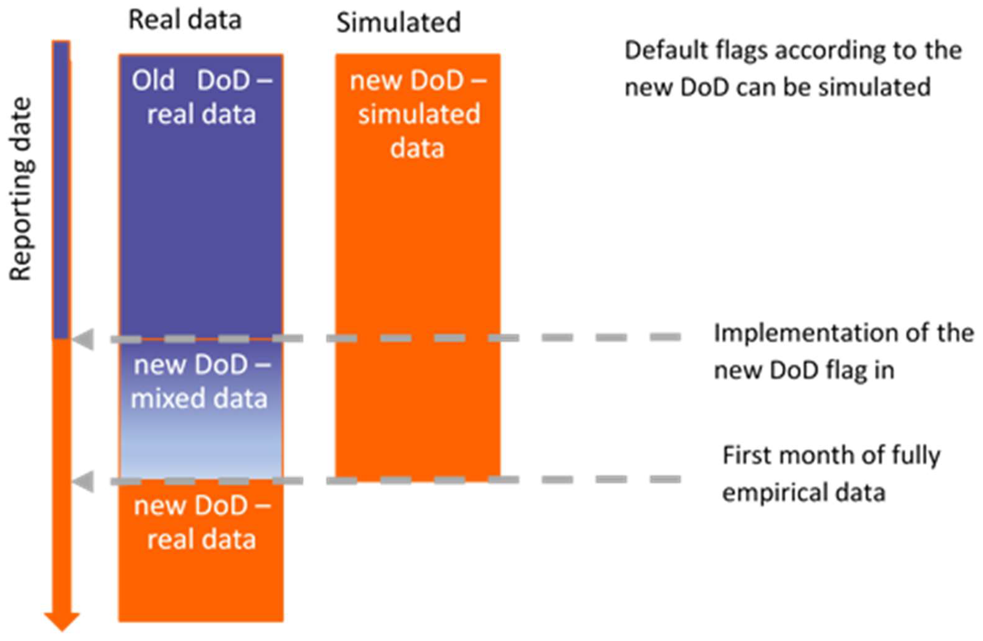
Data used in the process of recalibration and re-development of models can be simulated, empirical and mix type (see

Table 1. Types of data utilized.

Model	Re-calibration of IRB models (end of year 2021)	Re-development of models using new data (years 2022/2023)
PD	Default data—simulated Additional data—empirical	Simulated data (option of immediate redevelopment) Empirical data (redevelopment possible after 2 years of data collection)
LGD	Default data—simulated Collection data—real empirical data after default date	Empirical/mixed data, No simulated data

). Figure 1 presents how these types of data can be used. Before implementation of a new DoD flag in the system only simulated data on new DoD are available. After a sufficient DpD period post implementation there is new DoD empirical data available in the system. Both types of data can be used in re-calibration and re-development. Re-development on real empirical data will be only possible after two years period post implementation. Re-calibration must be undertaken on mixed data simulated and empirical. The only limitation is for LGD re-development because collection data are available only empirically; there is no simulation data for collections.

Steps of recalibration/re-development of models for credit risk parameters:

• Simulation of data concerning the new definition of default for different portfolios.
• Construction of Analytical Based Tables (ABTs) for model’s re-calibration process.
• Construction of codes for recalibration process automatization—model development.
• Construction of codes for validation process automatization—model validation.
• Re-calibration of LGD/CR, EAD/CCF parameters.

  ○

  Scaling factors.

  ○

  Regression models adjusting the old risk parameter to the new one.

• Re-development of models in case of negative back-test after re-calibration of models.

  ○

  Models including a-priori distributions (Bayesian approach).

  ○

  Parametric models.

  ○

  Non-parametric models.

• Validation of the model’s re-calibration/re-development process.

3.1. Probability of Default PD—Model Recalibration

There are two approaches for PD model recalibration—one based on scaling factors and the alternative one based on model estimation.

The first approach is based on scaling factors as conservative add-on. We have two or more different scaling factors proposed in this approach. A basic scaling factor assumes that new default rate can be re-scaled proportionally for particular risk grades, segments by proportional change of PD using the following formula, assuming Default Rate (DR) as empirical realization of PD:

$$P{D}_{new}=P{D}_{old}·f,f=\frac{D{R}_{new}}{D{R}_{old}},$$

(1)

where: f—scaling factor, PD—probability of default, DR—default rate.

When scaled probability takes a value out of the accepted range, then another approach is needed. One of them can be a logit scaling factor given by the following formula:

$$P{D}_{new}=\frac{f·P{D}_{old}}{1+\left(f-1\right)·P{D}_{old}},f=\frac{\frac{1-D{R}_{old}}{D{R}_{old}}}{\frac{1-D{R}_{new}}{D{R}_{new}}},$$

(2)

Of course, other scaling factors are also possible. They can be, for example, based on relations between neighboring rating grades.

Quite a different approach for calibration is based on the estimation of a new model. There are, of course, some options such as logit regression or the Bayesian approach. As an alternative to regression the non-parametric model can be estimated. In that case we need non-parametric model based on PD curve on rating scale grades.

For the redevelopment approach a Bayesian approach could be considered that would require prior information on simulated or mixed data, and likelihood based on real data for the new DoD.

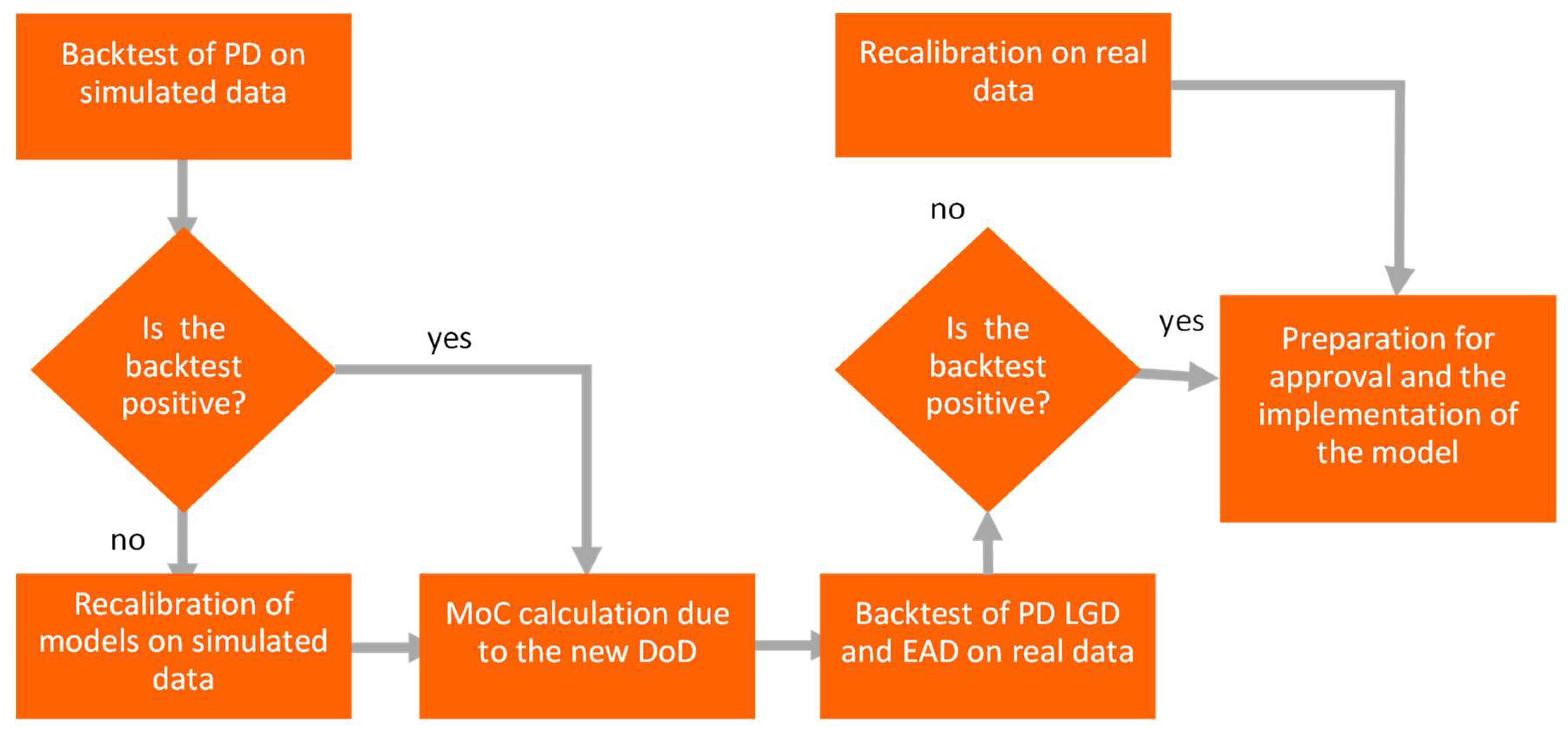
For built models it is not recommended to have calibration separate for rating grades, rather for the model level. In such situation the lack of PD monotonicity is observed, and additional algorithms are required to maintain monotonicity. To check the necessity of model re-calibration or re-development the backtest is performed. The consistency between model probability of default PD comparing to empirical default rate DR is backtested. As the first step, a backtest on simulated data is performed (see Figure 2) and if it is positive (not rejected), then MoC calculation is undertaken to adjust the new DoD. Only when it is positive and MoC is applied, a backtest on real data is performed and, if positive, the implementation phase is launched. If the backtest on real data is negative (rejected), recalibration on real data is performed. If the backtest on simulated data is negative, an additional step of recalibration on simulated data is performed.

3.2. Loss Given Default LGD—Model Recalibration

Backtesting, recalibration or redevelopment processes are different for LGD due to the limited size of population for modeling and more problematic use of historical simulated data. The LGD formula may contain many components that are estimated separately but the final formula depends on the specific debt collection process. The basic formula used for LGD is presented below.

LGD = (1 − CR)∙(1 − SRR)∙(1 − URR) + CR∙ L_cure,

(3)

where:

CR—cure rate,

SRR—secured recovery rate,

URR—unsecured recovery rate in relation to the reduced EAD with secured recoveries,

L_cure—the economic loss associated with cured cases expressed as a percentage of EAD.

Calibration of basic components of this LGD formula is based on:

• For the cure rate parameter (CR):

  ○

  scaling factor (including no-loss),

  ○

  logistic regression model,

  ○

  full recalibration using the Bayesian approach,

  ○

  recalibration using survival methods (with censored observations).

• For the secured and unsecured recovery rate (SRR, URR):

  ○

  calibration using the scaling factor,

  ○

  linear or non-linear regression model,

  ○

  full calibration using regression models including simultaneous calibration of both parameters.

The recalibration of LGD depends on the type of the new period of data available—if it is a downturn period or not (see Figure 3).

If the period cannot be qualified as downturn, a backtest approach with a scaling factor is applied and if it is positive (not rejected), it is the end of recalibration. If it is not positive (rejected), a full recalibration based on the Bayesian approach is applied. More sophisticated, hierarchical Bayesian models for LGD are applied instead of two combined models. The first model is used to separate all positive values from zeroes and the second model is than used to estimate only positive values (Bijak and Thomas 2015; Papouskova and Hajek 2019). If the backtest is not positive, the conservative MoC is needed. If the period is qualified as downturn, a backtest is applied on real data for LGD downturn. If it is positive, the recalibration ends. If the backtest is not positive (rejected), a conservatism option for LGD downturn is applied.

Understanding the data is crucial in the case of LGD recalibration. As shown in Figure 4, the data period for the new DoD may be different than for the old DoD in terms of its length and start date. The worst-case scenario is when the new default date is several months after the old default date. This is because all recoveries and other LGD components have been observed from the old default date, but the modeling or recalibration process requires them to be used right after the new default date. Since default entry and exit dates can be simulated on historical data this does not apply to the recovery process. The challenge for a modeler is to determine which data should be used—the old observer recoveries that are inconsistent with the new default date or only those that are observed right after the new default date. The answer is not unambiguous but in the case of significant differences between the old and new recoveries the former should be taken into account. The choice of using observed recoveries beyond the old default date may be justified as the recovery process does not change in most cases after the introduction of the new DoD.

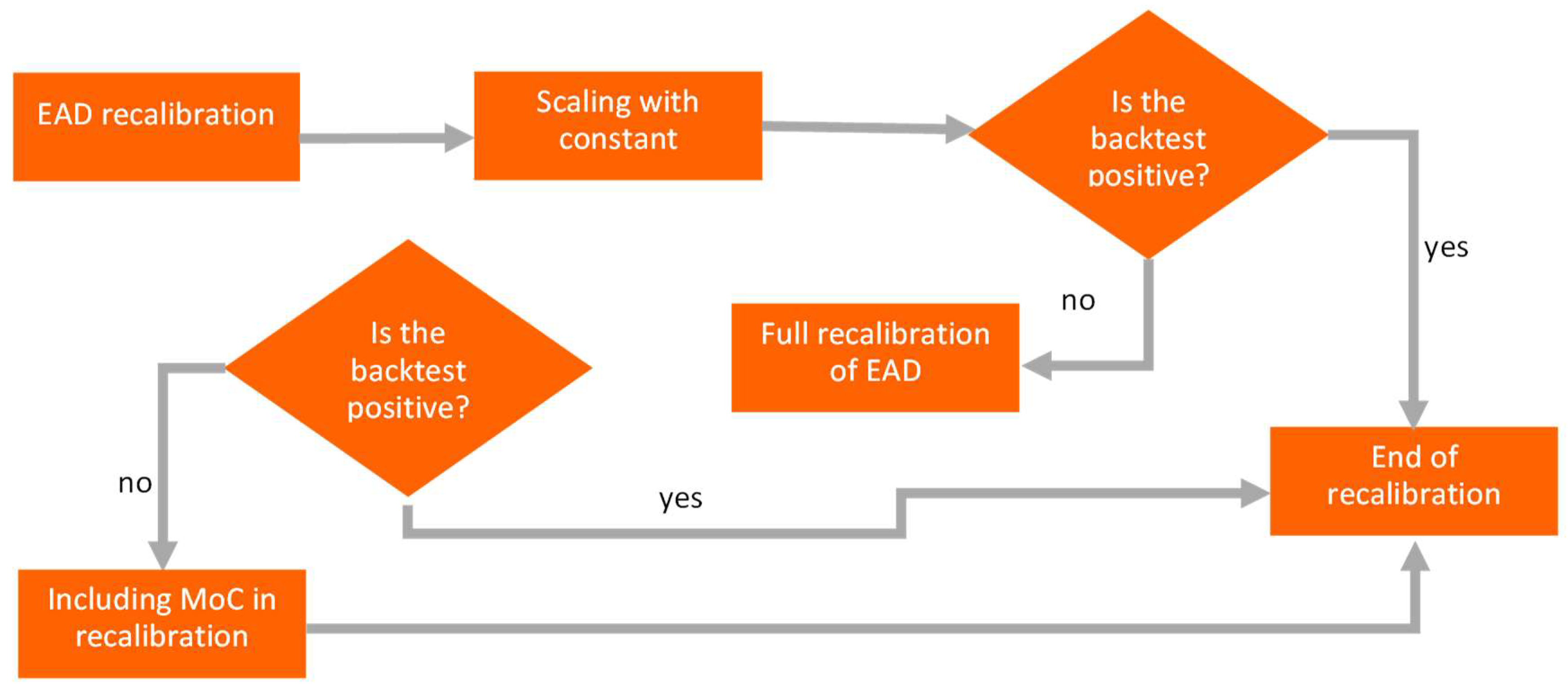
3.3. Exposure at Default EAD—Model Recalibration

The EAD recalibration is based on constant. We have four possible scenarios as indicated below:

Scenario	Parameters Description
1	Exposure below limit
2	Exposure equal limit or above (>0)
3	Exposure positive, limit 0
4	Exposure and limit equal 0

For the above scenarios adjustment coefficients are defined. Those coefficients equal the relation between the previous and new parameter such as:

• credit conversion factor (CCF) in the first case;
• the ratio of limit in the observation date for a facility to all limits for all facilities in a sample in the second case;
• the ratio of exposure at observation date for a facility to all exposures for all facilities in a sample in the third case;
• constant value estimated on the sample in the fourth case.

Those factors usually equal average factors for a portfolio, as the following formula indicates in the first case:

$$ad{j}_{factor}=\frac{CC{F}_{new}}{CC{F}_{old}},$$

(4)

where $CC{F}_{new},CC{F}_{old}$ are conversion factors based on the new and old definition of default.

The process of EAD recalibration is shown in Figure 5. If scaling with constant gives a positive (not-rejected) backtest result, we end recalibration. If the result is negative (rejected), a full recalibration is applied. When the full recalibration still gives a negative backtest (rejected), then conservative MoC is applied.

3.4. The Bayesian Approach in PD Recalibration

When the backtest fails on the recalibrated model, it is necessary to rebuild a new model. The redevelopment should take into account both simulated and empirical data. There is no need to use more sophisticated models in terms of advanced analytics, but rather to ensure clear data preparation and use models that take into account all information available when rebuilding the model. At the early stage of collecting data for new defaults, empirical data is not large enough to build a model on its own. A suitable methodology for both simulated and empirical data is the Bayesian approach, which can be used for different data sources, even if some data sets are small (Surzhko 2017; Zięba 2017). An additional advantage of Bayesian approach is the possibility of using expert knowledge not contained directly in the data (Simonian 2011). When the PD model is rebuilt, the simulated data is combined with the empirical data. From the purer statistical point of view the final PD is based on posterior distribution which is the product of the prior information and the likelihood.

First some basic assumptions must be introduced:

• PD_sim—PD estimated on simulated data;
• PD_emp—PD estimated on empirical data, at start this population is much smaller than the simulated one;
• prior information comes from simulated data;
• likelihood comes from empirical data;
• posterior distribution is a combination of prior distribution and likelihood;
• final PD is based on posterior distribution characteristics;

In general, the Bayesian approach can be applied when simulated PD_sim does not pass the alignment on empirical data, which means that there is no match between simulated PD_sim and empirical PD_emp.

The estimated parameter is PD_sim on simulated data with additional information from empirical data:

$$\pi (P{D}_{sim}|P{D}_{emp})\propto \pi \left(P{D}_{sim}\right)·f(P{D}_{emp}\left|P{D}_{sim}\right),$$

(5)

where:

• $\pi (P{D}_{sim}|P{D}_{emp})$—is the posterior distribution under condition of PD_emp,
• $\pi \left(P{D}_{sim}\right)$—is the prior distribution,
• $f(P{D}_{emp}|P{D}_{sim})$—likelihood—conditional distribution of $P{D}_{emp}$ parameter under the condition of $P{D}_{sim}$.

All simulations can be performed using Markov Chain Monte Carlo (MCMC) methods. The main advantages of this approach are as follows (Robert 1994):

• The Bayesian approach fits estimate parameters very well with the use of knowledge from different data sources, both internal and external. However, before applying the Bayesian technique the following problems should be solved. The choice of prior distribution for PD simulated. The prior should be based on portfolio characteristics and the uncertainty in data;
• The choice of MCMC technique, such as Gibbs sampling, Hastings–Metropolis or other when explicit posterior cannot be found;
• The possibility of including other prior information that is not derived from the data such as future macroeconomic conditions in some selected industries;
• The possibility of calculating confidence intervals for PD and using a more conservative estimator.

4. PD Recalibration—Application on Real Data

Application on real data sample was based on selected portfolio of retail mortgages loans for one of European banks. Time frame for the sample was restricted to years 2008–2020. The development sample for the PD model includes around 15K observations, where 4K observations come from the period of simulated defaults and 11K from the period of empirical defaults. This sample was drawn from the population including around 132K observations by selecting all defaults and drawing non-default cases with probability less than 0.1. Hence, the development sample was reweighted. PD model was built on the reweighted population because the total population includes too many “good” customers for modeling purpose, that is the inclusion of too many observations could lead to numerical problems in estimation and is more time consuming. Another reason to weigh population in processes of model building is the better learning of the risk profile by increasing the share of “bad” customers. The default rate in the entire population before drawing observations for the modeling process was 1.75% and 1.52% for simulated and empirical cases, respectively. The stability of both the default rate and the arrears amount (maximum and the average arrears for the facility) is presented in the

Table 2. Default rate and arrears amount.

Year	Count	Default Rate	Arrears Max [Thousand EUR]	Arrears Average [Thousand EUR]
2008	6939	0.72%	10.59	6.36
2009	8973	0.57%	15.93	3.32
2010	7502	0.72%	14.29	2.64
2011	6889	1.32%	19.29	4.82
2012	7860	2.01%	19.21	4.19
2013	8993	2.62%	26.60	7.72
2014	9774	2.34%	32.68	7.00
2015	10,725	2.45%	28.64	8.52
2016	12,545	2.18%	22.42	6.40
2017	16,832	1.73%	36.84	20.93
2018	3290	1.52%	19.81	6.21

. The arrears amount means the total outstanding of the customer after default moment.

Simulated defaults were selected within the period 2008–2018 but empirical defaults were more relevant after 2019. The sample was split into two independent subsamples for simulated and empirical defaults. While the model was built on the whole sample, including both the simulated and empirical defaults, the recalibration was mainly performed on simulated data with the additional use of empirical defaults according to the Bayesian methodology.

The process of recalibration includes the following steps:

• Building the new PD model on the joint population for simulated and empirical defaults, i.e., a mixed population. The model is built with use of logistic regression;
• Calculation of Long Run Average (LRA) on the simulated data. LRA is the average of default rates calculated within the given period of time;
• Adjusting LRA through the Bayesian methodology, which combines both the simulated and empirical data. The role of empirical data is to adjust the LRA calculated on the simulated data;
• Final recalibration of the PD parameter estimated in the 1st step at the facility level according to the posterior mean calculated at the step 3. The final step is also performed with Bayesian approach.

Summarizing the above algorithm, the Bayesian approach was used both to find the posterior estimators and final recalibration of the model but was applied to two different models.

The PD model was built on a population of around 15K observations and a default rate of 0.017424. The entire data set contained around 400 risk drivers that had been previously selected due to their business intuitiveness and high data quality. The model estimation procedure was based on logistic regression with a stepwise selection method assuming that the p-value for entering the variable into the model was 0.05 and the p-value for remaining in the data was 0.001. The final model was based on around 10 variables with the p-value for the test of significancy of the coefficient at the variable not higher than 0.004. The estimation procedure was performed in SAS. Ultimately, PD was explained by some transformations of the following variables:

-

Absolute breach in the past;

-

Relative breach in the past;

-

Maximum DpD in the past;

-

Amount of maximum arrears in the past;

-

Total obligations;

-

The age of the customer;

-

Account balance.

The quality of the model measured with Area Under ROC Curve (AUC) is 0.9. The model was built on the reweighted population to increase the default rate. Both simulated and empirical data were included in the population, but the defaults were underrepresented by the reduction in the population of “good” customers. The abovementioned reasons require a recalibration process, but the latter require more sophisticated methods such as Bayesian approach.

The next step after building the model was the choice of the calibration methodology. The starting point in this process was the calculation of Long Run Average of DR (LRA) on the simulated data, which was 0.017499, while the standard deviation of its estimator was 0.131123. An attempt was made to include empirical data that turned out to be too small to estimate risk parameters and the Bayesian methodology was used. The Bayesian approach can be considered as an improvement of LRA using empirical data that was initially calculated on the simulated data. In general, the PD calculated on simulated data is prior information, but the PD calculated on empirical data provides real information that is not biased by the simulation process. Nevertheless, the empirical population is too small to recalibrate the model. According to the Bayesian methodology, the following assumptions (6) and (7) were made and incorporated into the MCMC SAS procedure:

$$P{D}_{sim}~N\left(E\left(LR{A}_{sim}\right),std\left(LR{A}_{sim}\right)\right),$$

(6)

where: PD_sim is a random variable normally distributed around E(LRA_sim).

E(LRA_sim) and std(LRA_sim) are the expected value of LRA and standard deviation of LRA, respectively, calculated on the simulated data.

The above assumptions related to the distribution of PD_sim is directly derived from the historical data. The distribution of the variable PD_sim is considered as prior distribution. This is the case where prior distribution is more objective as it is based on historical data. We used many different prior distributions which are allowed by SAS MCMC procedure and the final posterior results were very similar which further proves robustness of the posterior estimators.

The likelihood which is the distribution of the PD_emp parameter on the empirical data is the binomial distribution with the number of trials that equals the number of observations n_emp in the empirical data and the probability of success equals the PD_sim calculated on the simulated data. Hence, the likelihood can be viewed as a conditional distribution of the PD parameter on empirical data given the PD_sim calculated on the simulated data is defined as follows:

$$P{D}_{emp}|P{D}_{sim}~B\left(n_{emp}, P{D}_{sim}\right),$$

(7)

where: PD_emp is a random variable binomially distributed (Joseph 2021) with parameters n_emp and PD_sim.

Based on the above two distributions of prior and likelihood, the characteristics of posterior density were calculated using the MCMC procedure and the following results for the posterior expected value and posterior standard deviation were obtained:

$$\begin{gathered} P{D}_{sim|emp}=E[P{D}_{sim}|P{D}_{emp}]=0.0155 \\ s[P{D}_{sim}|P{D}_{emp}]=0.0021 \end{gathered}$$

The obtained posterior mean $P{D}_{sim|emp}$ of 0.0155 is the new calibration purpose.

The following table (see

Table 3. PD estimator results.

Simulated Data (Prior)	Development Data	Empirical Data	Posterior
0.017499	0.017424	0.015198	0.0155

) summarizes all considered PD estimators obtained on the simulated data, empirical data, development data and the Bayesian calculation as a posterior mean.

The final recalibration of the PD parameter was based on the new recalibration purpose using the logistic Bayesian model. The default flag shows binary distribution with the expected value that equals the unknown calibrated PD (PD_cal) depending on the simulated PD (PD_sim) and two additional parameters a and b as follows:

$$\begin{gathered} D~Bin\left(f(P{D}_{sim},a,b\right)\left|P{D}_{emp}\right) \\ P{D}_{cal}=f\left(P{D}_{sim},a,b\right)=f(a·\ln \left(\frac{P{D}_{sim}}{1-P{D}_{sim}}\right)+b) \end{gathered}$$

(8)

where f is the logistic function.

Parameters a and b are hyperparameters normally distributed with the following mean and standard deviation:

$$\begin{gathered} a~N\left(1,{\sigma }_a\right) \\ b~N\left(\ln \left(\frac{P{D}_{sim|emp}}{1-P{D}_{sim|emp}}\right)-\ln \left(\frac{D{R}_{mod}}{1-D{R}_{mod}}\right),{\sigma }_b\right) \end{gathered}$$

(9)

where $D{R}_{mod}$ = 0.017424 is the default rate on the modeled data set.

The concept of the expected value for parameter b is that it should be positive when $P{D}_{sim|emp}$ is higher than $D{R}_{mod}$ but otherwise negative bearing in mind that this is an additive part to the log odds. The formula for b parameter is the main point in this Bayesian model to include the information about the posterior mean to which to calibrate the model.

Both standard deviations ${\sigma }_a$ and ${\sigma }_b$ have standard deviation uniformly distributed over the interval (0,1). The upper value of the interval is based on previous experiments with data. An alternative approach to find estimators a and b is to use simple non-Bayesian regression logistic. The Bayesian approach is key in the previous step to find the posterior mean, but here it only serves as a consistent methodology and is not needed for finding the final recalibration formula. On the other hand, it can be easily extended by providing a greater external knowledge of the estimated parameters. Therefore, it can be taken as a pattern for the further calculations on other data, which is very flexible. Ultimately, posterior averages for a and b were calculated, respectively (see

Table 4. Posterior parameters for the Bayesian approach.

Parameter	Mean	STD	95% HPD Interval
a	0.88	0.0896	0.7229	1.0791
b	−5.4135	0.2399	−5.8676	−4.9243
sigma_a	0.4013	0.298	0.00168	0.9242
sigma_b	0.9423	0.0535	0.8326	1

).

In order to obtain the final PD estimation formula, the logistic regression Equation (8) for the entire PD was applied. Additionally, the PD calibrated without the Bayesian method was calculated for comparison (see

Table 5. Parameters calculated without the Bayesian approach.

Parameter	Mean	STD	95% HPD Interval
a	1.1087	0.0192	1.0736	1.1498
b	−5.9081	0.0512	−6.0129	−5.8132

). It is worth mentioning that the simple logistic regression model based on the Equation (8) but without taking into account parameter distributions can be built with use of the following weights for all observations to adjust the mean default rate to posterior mean. In case of Bayesian approach weights were not needed as b parameter in the model plays the role of such adjustment.

$$w=\frac{P{D}_{sim|emp}}{1-P{D}_{sim|emp}}·\frac{1-D{R}_{mod}}{D{R}_{mod}}$$

(10)

All PD’s distributions for the raw PD obtained from the model built on the reweighted sample, PD calibrated without the Bayesian methodology and PD using the Bayesian approach are presented below in Figure 6a,b.

Summarizing the classic approach to building the logistic regression model as the final calibration formula is possible only with introducing weights for observations; the Bayesian approach does not require weights but an appropriate definition of distributions for regression parameters.

5. Conclusions and Discussion

Recent changes in economy caused by COVID pandemic (Batool et al. 2020) had an impact on sharing economy but also a significant impact on the banking sector. Recent changes in Industry 4.0 were also not neglectable for Banking 4.0 (Mehdiabadi et al. 2020). Significant regulatory changes imposed by regulatory authorities followed those changes.

The regulatory requirements related to the change in the definition of default have significant impacts from a banking perspective, with the most material one on credit risk modeling. From a methodological point of view, all provisioning IFRS9 and capital IRB regulatory models need recalibration. At the same time, empirical evidence that is obtained when the new definition is applied to real portfolios is still being collected. In this context, the paper provides an overview of the main implications deriving from the regulation in different risk management areas (e.g., data, default definition, implementation, identification) and discusses a methodological proposal for IRB modeling recalibration to address the current challenges. The idea is to leverage the Bayesian approach for PD recalibration by retrieving information from both simulated and empirical data (e.g., a priory and a posteriori distributions). As discussed in the methodological section, this mathematical approach seems to be a promising solution to building a robust framework in the current phase and addressing the gaps. In our plans for future research, we foresee an empirical study to test how the proposed methodology can perform in different credit risk modeling contexts.

Finally, we used the Bayesian approach in two steps: the first basic approach is to calculate the LRA on both simulated and empirical data. In addition, we used the same approach for the final model calibration to the posterior LRA. In summary, the Bayesian approach result for the PD LRA was slightly lower than the one calculated based on classical logistic regression (Figure 6). It also decreased for the historically observed LRA (Table 3) that included the most recent empirical data. The Bayesian methodology was used to make the LRA more objective, but it also helps to better align the LRA not only with the empirical data but also with the most recent ones. It allows us to consider the LRA as a random variable, where its variance tells us more about the significance of the point estimation. The greater the variance, the more empirical data need to be included in the calculation of the end value. When comparing the standard deviation of the LRA calculated on the simulated data, which is 0.131123 with the mean of 0.017499, there is still room to improve this estimator with less volatile data, such as empirical with the mean LRA of 0.0155 and much lower standard deviation of 0.00214. To sum up, it is a unique approach to statistical modeling that can combine different information, even expertise, not covered by historical data. Moreover, it can be applied to both LGD and EAD, but PD is preferred as the starting point. Promising results for PD were also obtained by (Wang et al. 2018) with ARIMA model results as prior for Bayesian approach confirming outperformance comparing to frequentist approach.

From a practical point of view, using the Bayesian approach can significantly decrease the capital requirements, thus making savings for organization from managerial perspective. Close to the empirical values, the calculations of capital adequacy and provisions are as more precise, keeping of course regulatory requirements fulfilled.

A weakness of the proposed approach, however mitigated, is due to normal distribution assumption. Some ideas for future research rely on further investigation of the Bayesian approach, but perhaps for small samples or other parameters as well. This approach seems also promising for IFRS 9 lifetime parameter estimation.