Gain-Preserving Data-Driven Approximation of the Koopman Operator and Its Application in Robust Controller Design

Abstract

In this paper, we address the data-driven modeling of a nonlinear dynamical system while incorporating a priori information. The nonlinear system is described using the Koopman operator, which is a linear operator defined on a lifted infinite-dimensional state-space. Assuming that the ${\mathcal{L}}_2$ gain of the system is known, the data-driven finite-dimensional approximation of the operator while preserving information about the gain, namely ${\mathcal{L}}_2$ gain-preserving data-driven modeling, is formulated. Then, its computationally efficient solution method is presented. An application of the modeling method to feedback controller design is also presented. Aiming for robust stabilization using data-driven control under a poor training dataset, we address the following two modeling problems: (1) Forward modeling: the data-driven modeling is applied to the operating data of a plant system to derive the plant model; (2) Backward modeling: ${\mathcal{L}}_2$ gain-preserving data-driven modeling is applied to the same data to derive an inverse model of the plant system. Then, a feedback controller composed of the plant and inverse models is created based on internal model control, and it robustly stabilizes the plant system. A design demonstration of the data-driven controller is provided using a numerical experiment.

1. Introduction

In recent years, data-driven modeling of dynamical systems has become an active and central theme in various research communities such as dynamical systems theory [1], control engineering [2], etc. The main aims of this modeling are to understand, analyze, and control the dynamical system in an efficient and reliable manner. To further improve the efficiency and reliability, there have been many trials on data-driven modeling while incorporating a priori known information on the dynamical system. Some examples of the a priori known information include the properties of linear dynamical systems such as stability [3], dominant eigen-mode [4,5], steady-state response [6,7], passivity [8,9], frequency response [10], system moment [11], etc. The general aim of this paper is to extend data-driven modeling techniques utilizing such a priori known information for linear systems to nonlinear system modeling. In particular, we address the problem of data-driven modeling of nonlinear dynamical systems while incorporating the input–output gain of dynamical systems, which plays central roles in robustness analysis and robust controller design [12].

The Koopman operator is a linear operator defined on the lifted infinite-dimensional state-space and is utilized for analyzing complex dynamical systems. Motivated by its high ability to express nonlinearity, data-driven finite-dimensional approximation of the operator has been studied and applied not only in system analysis [13,14,15] but also in control system design [16,17,18,19,20,21,22,23,24,25,26]. In this paper, a nonlinear dynamical system is described using the Koopman operator, and its data-driven approximation is addressed. Assuming that the input–output gain of the system is available in addition to system operating data, the data-driven approximation of the Koopman operator while preserving information on its gain, namely gain-preserving data-driven modeling, is formulated. Then, an efficient method for resolving the problem is presented based on the work of References [15,27].

The modeling method is applied to data-driven feedback controller design based on internal model control (IMC [28,29]). IMC is a model-based control technique in which a plant model is directly embedded as part of the controller. Since IMC is compatible with data-driven modeling, there have been various work on data-driven IMC design. See, for example, the work in References [30,31,32,33]. The main drawback of conventional data-driven IMC is the fragility of the controlled system. There inevitably exists a modeling error in the plant model that may cause performance degradation and destabilization of the controlled system, in particular, when rich data is not available for modeling. In this paper, we address the data-driven design of a robust and reliable controller based on IMC in the following manner. First, we address forward modeling of the plant: a data-driven modeling method is applied to the operating data of a plant system to derive the plant model as an approximated Koopman operator. Secondly, we address backward modeling of the plant: gain-preserving data-driven modeling is applied to the same data to derive an inverse model of the plant system. Then, the two models are used to form an IMC-based feedback controller that robustly stabilizes the plant system.

The remaining parts of this paper are organized as follows. In Section 2, we review the theory on the Koopman operator, the stability concept for input–output dynamical systems, and IMC. Section 3 is devoted to the gain-constrained data-driven approximation of the Koopman operator. The approximation problem is formulated, and a numerically efficient algorithm is presented. In Section 4, the gain-constrained approximation is applied to the IMC design, and robust stabilization of the overall control system is achieved. Section 5 shows a demonstration of the proposed data-driven robust IMC.

Notation: ${\parallel M\parallel }_F$ represents the Frobenius norm of matrix M. In addition, $\mathrm{He}\left(N\right)$ represents $\mathrm{He}\left(N\right)=N+N^{\top }$ for square matrix N. The positive and negative definiteness of matrix M are denoted by $M\succ 0$ and $M\prec 0$, respectively.

2. Preliminaries

2.1. Koopman Operator and Its Data-Driven Approximation

In this subsection, we consider a nonlinear dynamical system described by the discrete-time state equation:

$$\begin{array}{c}\hfill \mathcal{S}:\left\{\begin{array}{cc}\hfill x(k+1)& =f\left(x\left(k\right),u\left(k\right)\right),\hfill \\ \hfill y\left(k\right)& =g\left(x\left(k\right)\right),\hfill \end{array}\right.\end{array}$$

(1)

where k is the discrete time, $x\in {\mathbb{R}}^n$ is the state, $u\in {\mathbb{R}}^m$ is the input, $y\in {\mathbb{R}}^l$ is the output, and $f(·):{\mathbb{R}}^{n+m}\to {\mathbb{R}}^n$ and $g(·):{\mathbb{R}}^n\to {\mathbb{R}}^l$ are the nonlinear functions. Nonlinear system $\mathcal{S}$ is expressed by the Koopman operator, and its data-driven approximation is stated.

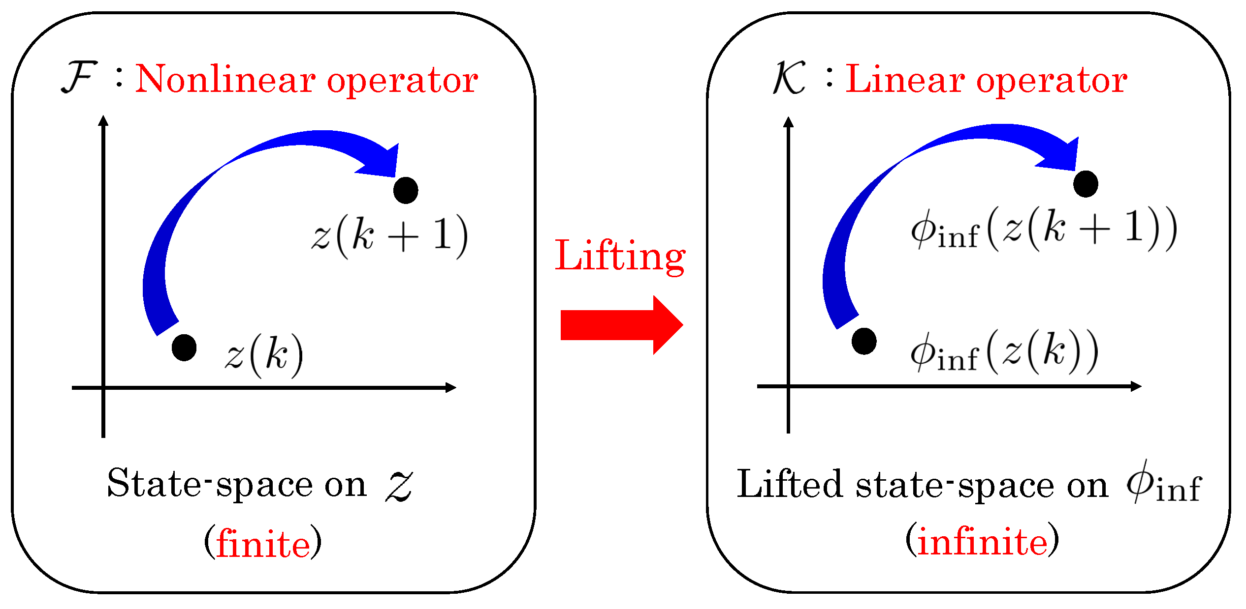
2.1.1. Koopman Operator

Let z denote the extended state:

$$\begin{array}{c}\hfill z:=\left[\begin{array}{c}x\\ u\end{array}\right]\in {\mathbb{R}}^{n+m},\end{array}$$

we define nonlinear operator $\mathcal{F}$ by

$$\begin{array}{cc}\hfill \mathcal{F}\left(z\right)& :=\left[\begin{array}{c}f(x,u)\\ \mathcal{T}\left(u\right)\end{array}\right],\hfill \end{array}$$

where $\mathcal{T}$ is the time-shift operator:

$$\begin{array}{cc}\hfill \mathcal{T}\left(u\right(k\left)\right)& :=u(k+1).\hfill \end{array}$$

Then, the time evolution of z is described by

$$\begin{array}{c}\hfill z(k+1)=\mathcal{F}\left(z\right(k\left)\right).\end{array}$$

Now, we introduce the Koopman operator. To this end, let ${\varphi }_{\inf }\left(z\right)$ denote the infinite-dimensional lifting function described by

$$\begin{array}{c}\hfill {\varphi }_{\inf }\left(z\right)=\left[\begin{array}{c}{\varphi }_1\left(z\right)\\ {\varphi }_2\left(z\right)\\ ⋮\end{array}\right].\end{array}$$

Then, the Koopman operator, denoted by $\mathcal{K}$, is defined as

$$\begin{array}{c}\hfill \mathcal{K}\left({\varphi }_{\inf }\left(z\right)\right):={\varphi }_{\inf }\left(\mathcal{F}\left(z\right)\right).\end{array}$$

The time evolution of ${\varphi }_{\inf }\left(z\right)$ follows:

$$\begin{array}{c}\hfill {\varphi }_{\inf }\left(z(k+1)\right)=\mathcal{K}\left({\varphi }_{\inf }\left(z\left(k\right)\right)\right).\end{array}$$

(2)

Note that the Koopman operator is a linear operator defined on the infinite-dimensional lifted state space, while expressing the nonlinear dynamics described by (1). Figure 1 provides a sketch of nonlinear operator $\mathcal{F}$ on the state space and Koopman operator $\mathcal{K}$ on the lifted state space.

Figure 1. Nonlinear operator $\mathcal{F}$ on state space and Koopman operator $\mathcal{K}$ on lifted state space.

2.1.2. Approximation of the Koopman Operator

Due to its infinite-dimensionality, the Koopman operator is not tractable for numerical analysis, simulation, and system design. In this subsection, the finite-dimensional approximation of the operator is addressed. To this end, we define $N_{\varphi }$-dimensional lifting function $\varphi \left(z\right):{\mathbb{R}}^{n+m}\to {\mathbb{R}}^{N_{\varphi }}$ as

$$\begin{array}{c}\hfill \varphi \left(z\right)=\left[\begin{array}{c}{\varphi }_1\left(z\right)\\ ⋮\\ {\varphi }_{N_{\varphi }}\left(z\right)\end{array}\right]\in {\mathbb{R}}^{N_{\varphi }}.\end{array}$$

Furthermore, we let $\mathcal{A}\in {\mathbb{R}}^{N_{\varphi }\times N_{\varphi }}$ be a finite-dimensional matrix that approximates operator $\mathcal{K}$. In other words, $\mathcal{A}$ is found such that $\parallel \mathcal{A}\varphi \left(z\right)-\varphi \left(\mathcal{F}\right(z\left)\right)\parallel$ is sufficiently small for some normal sense. With this $\mathcal{A}$, we have the following expression:

$$\begin{array}{c}\hfill \varphi \left(z\right(k+1\left)\right)\approx \mathcal{A}\varphi \left(z\right(k\left)\right),\end{array}$$

(3)

which approximately expresses the time evolution of ${\varphi }_{\inf }\left(z\left(k\right)\right)$, described in (2).

We address the data-driven approximation of $\mathcal{K}$, i.e., the estimation of $\mathcal{A}$ using the data of time sequence $\left\{z\right(k\left)\right\}$. In particular, we aim to construct an input-linear model that approximates (3). To this end, we further specialize the class of lifting function $\varphi \left(z\right)$ in the following form:

$$\begin{array}{c}\hfill \varphi \left(z\right)=\left[\begin{array}{c}\psi \left(x\right)\\ u\end{array}\right]\in {\mathbb{R}}^{N+m},\end{array}$$

where $\psi \left(x\right):{\mathbb{R}}^n\to {\mathbb{R}}^N$ is the N-dimensional lifting function given by

$$\begin{array}{c}\hfill \psi \left(x\right)=\left[\begin{array}{c}{\psi }_1\left(x\right)\\ ⋮\\ {\psi }_N\left(x\right)\end{array}\right]\in {\mathbb{R}}^N,\end{array}$$

and $N+m=N_{\varphi }$ holds. Let matrix $\mathcal{A}$ be partitioned as

$$\begin{array}{c}\hfill \mathcal{A}=\left[\begin{array}{cc}A& B\\ *& *\end{array}\right]\in {\mathbb{R}}^{(N+m)\times (N+m)},\end{array}$$

where $A\in {\mathbb{R}}^{N\times N}$ and $B\in {\mathbb{R}}^{N\times m}$. It follows from (3) that the the time-evolution of $\psi \left(x\right)$ is expressed by

$$\begin{array}{c}\hfill \psi \left(x\right(k+1\left)\right)\approx A\psi \left(x\right(k\left)\right)+Bu\left(k\right).\end{array}$$

In addition, we address the approximation of the output equation in (1) by

$$\begin{array}{c}\hfill y\left(k\right)\approx C\psi \left(x\right(k\left)\right),\end{array}$$

where $C\in {\mathbb{R}}^{l\times N}$. For simplicity of notation, we let $\psi \left(k\right)=\psi \left(x\right(k\left)\right)$. Then, we obtain the lifted state-space equation defined on the functional space as

$$\begin{array}{c}\hfill {\mathcal{S}}_{\mathrm{koop}}:\left\{\begin{array}{cc}\hfill \psi (k+1)& =A\psi \left(k\right)+Bu\left(k\right),\hfill \\ \hfill y\left(k\right)& =C\psi \left(k\right).\hfill \end{array}\right.\end{array}$$

(4)

Model ${\mathcal{S}}_{\mathrm{koop}}$ of (4) approximately expresses the input–output behavior generated by nonlinear system $\mathcal{S}$. In this paper, model ${\mathcal{S}}_{\mathrm{koop}}$ is called the “Koopman model”. This paper addresses the data-driven modeling of ${\mathcal{S}}_{\mathrm{koop}}$ by estimating system matrices $\left(A,B,C\right)$.

2.1.3. Data-Driven Approximation of Koopman Operator

For simplicity of notation, we define the following data matrices based on the sequences of the input, output, and state of system $\mathcal{S}$.

$$\begin{array}{cc}\hfill U_k& :=\left[u\left(k\right)u(k+1)\cdots u(k+M-1)\right]\in {\mathbb{R}}^{m\times M},\hfill \\ \hfill Y_k& :=\left[y\left(k\right)y(k+1)\cdots y(k+M-1)\right]\in {\mathbb{R}}^{l\times M},\hfill \\ \hfill {\Psi }_k& :=\left[\psi \left(k\right)\psi (k+1)\cdots \psi (k+M-1)\right]\in {\mathbb{R}}^{N\times M},\hfill \\ \hfill {\Psi }_{k+1}& :=\left[\psi (k+1)\psi (k+2)\cdots \psi (k+M)\right]\in {\mathbb{R}}^{N\times M}.\hfill \end{array}$$

It should be noted that ${\Psi }_k$ and ${\Psi }_{k+1}$ are constructed by using the measured data on the state, denoted by $\left\{x\right(k),\dots ,x(k+M\left)\right\}$ through $\psi \left(k\right)=\psi \left(x\right(k\left)\right)$. The problem of data-driven Koopman modeling is formulated as follows.

Problem 1.

Given data matrices $(U_k,Y_k,{\Psi }_k,{\Psi }_{k+1})$, we solve the following optimization problem:

$$\begin{array}{c}\hfill \underset{A,B,C}{min}J(A,B,C),\end{array}$$

where $J(A,B,C)$ is given by

$$\begin{array}{c}\hfill J(A,B,C)={∥\left[\begin{array}{c}{\Psi }_{k+1}\\ Y_k\end{array}\right]-\left[\begin{array}{cc}A& B\\ C& 0\end{array}\right]\left[\begin{array}{c}{\Psi }_k\\ U_k\end{array}\right]∥}_F^2.\end{array}$$

(5)

The solution to Problem 1 is denoted by $(A^{†},B^{†},C^{†})$, which are estimates of the system matrices. It is assumed that ${\left[{\Psi }_k^{\top }{U}_k^{\top }\right]}^{\top }$ is of full row rank, which is a natural assumption when rich data are available for modeling. Then, $(A^{†},B^{†},C^{†})$ are uniquely determined.

2.2. ${\mathcal{L}}_2$ Stability

2.2.1. Definition of ${\mathcal{L}}_2$ Stability

In this subsection, we consider an input–output dynamical system such as system $\mathcal{S}$ of (1) and define the stability. The concept of the stability of input–output systems can be seen in the pioneering work [34]. In the following definitions, ${\left\{u\right\}}_0^k$ denotes input sequence $\left\{u\right(0),u(1),\dots ,u(k\left)\right\}$.

Definition 1.

Consider input–output system $y=\mathcal{S}u$. Then, system $\mathcal{S}$ is said to be ${\mathcal{L}}_2$ stable if there is positive constant $\gamma \in {\mathbb{R}}_{+}$ such that inequality

$$\begin{array}{c}\hfill \sum _{\tau =0}^{k}y{\left(\tau \right)}^{\top }y\left(\tau \right)\le \gamma \sum _{\tau =0}^{k}u{\left(\tau \right)}^{\top }u\left(\tau \right),\forall {\left\{u\right\}}_0^k\in {\mathcal{L}}_2,\forall k\in {\mathbb{Z}}_{+}\end{array}$$

(6)

holds.

Definition 2.

Suppose that input–output system $y=\mathcal{S}u$ is ${\mathcal{L}}_2$ stable. Then, the ${\mathcal{L}}_2$ gain of $\mathcal{S}$ is defined as

$$\begin{array}{c}\hfill {\parallel \mathcal{S}\parallel }_{{\mathcal{L}}_2}:=\underset{{\left\{u\right\}}_0^k\in {\mathcal{L}}_2}{sup}\sqrt{\sum _{\tau =0}^k\frac{y{\left(\tau \right)}^{\top }y\left(\tau \right)}{u{\left(\tau \right)}^{\top }u\left(\tau \right)}}.\end{array}$$

${\mathcal{L}}_2$ stability, given in Definition 1, can be said to be “finite-gain” ${\mathcal{L}}_2$ stability in a clearer manner. Characterization of the ${\mathcal{L}}_2$ gain for the Koopman model ${\mathcal{S}}_{\mathrm{koop}}$ of (4) is given in the following lemma. See, for example, the book in Reference [35] for details of its proof.

Lemma 1.

The following statements (i) and (ii) are equivalent.

(i)

$\parallel {\mathcal{S}}_{\mathrm{koop}}{\parallel }_{{\mathcal{L}}_2}\le \gamma$ holds.

(ii)

There exists symmetric matrix P such that the following inequalities hold.

$$\begin{array}{cc}\hfill & P\succ 0,\hfill \end{array}$$

(7)

$$\begin{array}{cc}\hfill & {\left[\begin{array}{cc}A& B\\ I& 0\end{array}\right]}^{\top }\left[\begin{array}{cc}P& 0\\ 0& -P\end{array}\right]\left[\begin{array}{cc}A& B\\ I& 0\end{array}\right]+\left[\begin{array}{cc}{C}^{\top }C& 0\\ 0& -{\gamma }^{2}I\end{array}\right]\prec 0.\hfill \end{array}$$

(8)

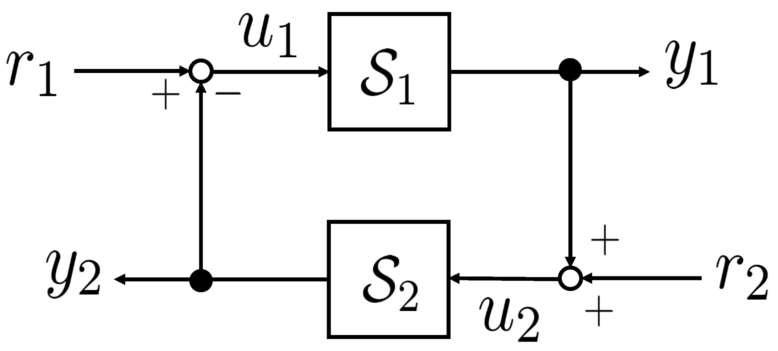
2.2.2. Stability Analysis for Feedback System

Stability analysis of the feedback systems is addressed in this section. We consider two input–output systems $y_i={\mathcal{S}}_i{u}_i$, $i\in \{1,2\}$ and their feedback connection, which is denoted by $\mathrm{FB}({\mathcal{S}}_1,{\mathcal{S}}_2)$ and illustrated in Figure 2. Then, the following lemma states the condition for ${\mathcal{L}}_2$ stability of the feedback system. See, for example, the work in Reference [34] for details.

Figure 2. Negative feedback interconnection of subsystems ${\mathcal{S}}_i$, $i\in \{1,2\}$.

Lemma 2.

Suppose that systems $y_i={\mathcal{S}}_i{u}_i$, $i\in \{1,2\}$ are ${\mathcal{L}}_2$ stable with ${\mathcal{L}}_2$ gain ${\gamma }_i$, $i\in \{1,2\}$, respectively. In other words, $\parallel {\mathcal{S}}_i{\parallel }_{{\mathcal{L}}_2}={\gamma }_i$, $i\in \{1,2\}$ hold. Then, feedback system $\mathrm{FB}({\mathcal{S}}_1,{\mathcal{S}}_2)$ illustrated in Figure 2 is ${\mathcal{L}}_2$ stable from $(r_1,r_2)$ to $(y_1,y_2)$ if

$$\begin{array}{c}\hfill {\gamma }_1{\gamma }_2<1\end{array}$$

(9)

holds.

Note that, in the lemma, any detailed model of subsystems ${\mathcal{S}}_i$, $i\in \{1,2\}$ such as the state-space model is not required for the stability analysis. The lemma plays an essential role of developing theory and applications of robust control. See, for example, the work in Reference [12].

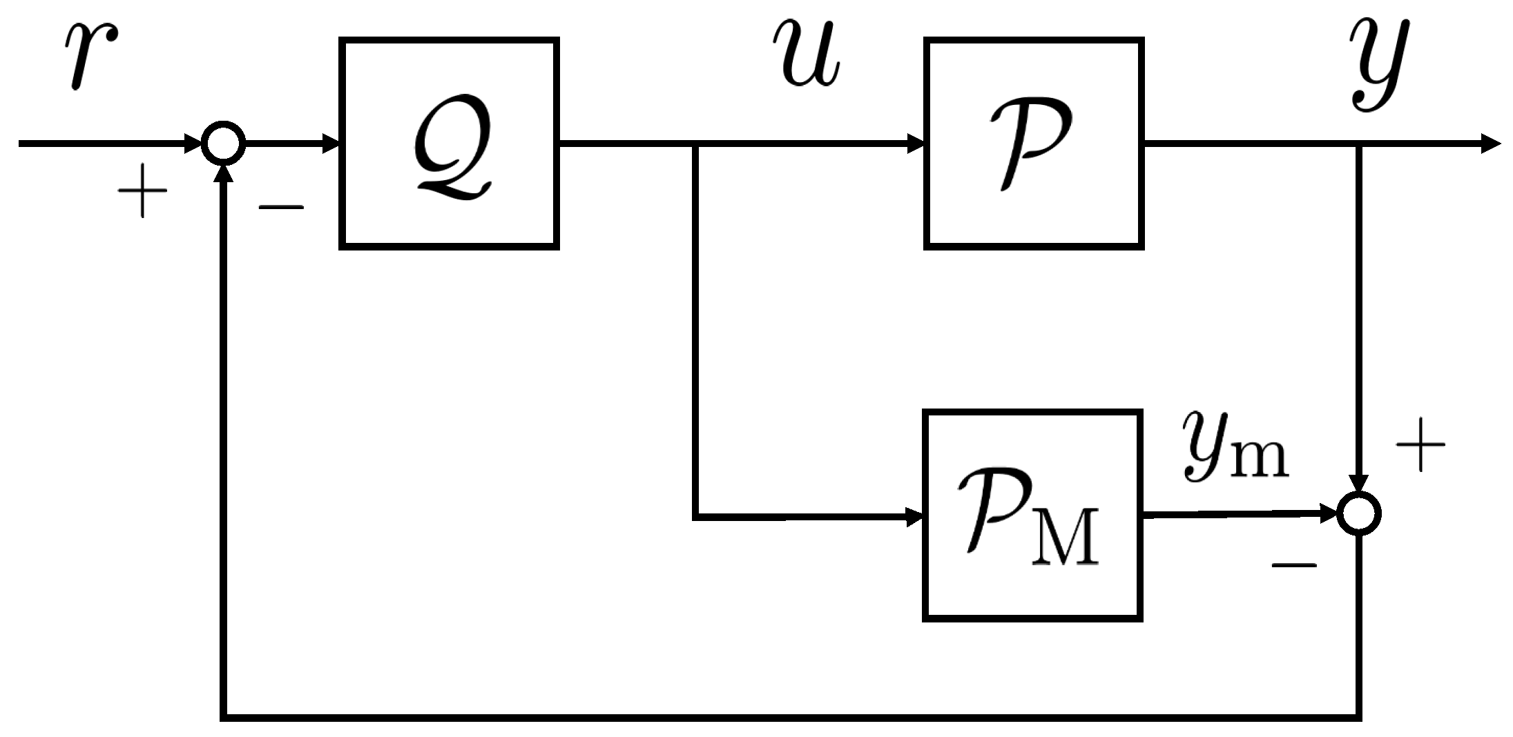
2.3. Internal Model Control

In this subsection, a feedback controller design called internal model control (IMC) is addressed. IMC is a model-based control technique and provides an effective, intuitive, and simple framework for analysis of the control system performance. See, for example, the pioneering works [28,29]. The structure of IMC is shown in Figure 3. In the figure, system $y=\mathcal{P}u$ is a nonlinear plant system to be controlled. Although the realization of $\mathcal{P}$ can be given by a state-space model such as $\mathcal{S}$ of (1), the discussion in this subsection is independent on system realization. System $y_{\mathrm{m}}={\mathcal{P}}_{\mathrm{M}}u$ is a model of plant system $\mathcal{P}$, and system $\mathcal{Q}$ is a filter to be designed. As illustrated in the figure, the positive feedback connection of ${\mathcal{P}}_{\mathrm{M}}$ and $\mathcal{Q}$ constitutes a controller. In the IMC scheme, the modeling error evaluated by the output of $\mathcal{P}$ and ${\mathcal{P}}_{\mathrm{M}}$ is fed back into the system. Then, the error is filtered by $\mathcal{Q}$ to generate control input u as

$$\begin{array}{c}\hfill u=\mathcal{Q}\left(r-(y-y_{\mathrm{m}})\right).\end{array}$$

Figure 3. A sketch of the feedback control system by IMC.

The overall control law is described by

$$\begin{array}{c}\hfill u={\left(I-\mathcal{Q}{\mathcal{P}}_{\mathrm{M}}\right)}^{-1}\mathcal{Q}(r-y).\end{array}$$

Some propositions for IMC are given as follows.

Proposition 1.

Suppose that ${\mathcal{P}}_{\mathrm{M}}=\mathcal{P}$ holds and that $\mathcal{P}$ and $\mathcal{Q}$ are ${\mathcal{L}}_2$ stable. Then, the overall control system in Figure 3 is ${\mathcal{L}}_2$ stable from r to y.

Proposition 2.

Suppose that ${\mathcal{P}}_{\mathrm{M}}=\mathcal{P}$ holds, that $\mathcal{P}$ is invertible, and that $\mathcal{P}$ and its inversion ${\mathcal{P}}^{-1}$ are ${\mathcal{L}}_2$ stable. Then, letting $\mathcal{Q}={\mathcal{P}}_{\mathrm{M}}^{-1}$, the overall control system in Figure 3 is perfectly controlled, i.e., $y\left(k\right)=r\left(k\right),\forall k$ holds.

Remark 1.

As implied in Proposition 2, the optimal design of filter $\mathcal{Q}$ is the inversion of plant model ${\mathcal{P}}_{\mathrm{M}}$. In the case that plant model $\mathcal{P}$ contains non-minimal phase elements, such as time delays and unstable zeros, the controller based on inverse model ${\mathcal{P}}_{\mathrm{M}}^{-1}$ is not realizable. To address this issue, a low-pass filter F is attached to inverse model ${\mathcal{P}}_{\mathrm{M}}^{-1}$ such that filter $\mathcal{Q}=F{\mathcal{P}}_{\mathrm{M}}^{-1}$ becomes (bi) proper and stable. Then, the controller composed of plant model ${\mathcal{P}}_{\mathrm{M}}$ and $\mathcal{Q}$ stabilizes the overall control system and achieves a high control performance. See the work in Reference [36] for more details.

3. Result 1: ${\mathcal{L}}_{\mathbf{2}}$ Gain-Preserving Data-Driven Modeling

In this section, we address the problem of data-driven modeling while preserving the ${\mathcal{L}}_2$ gain for nonlinear dynamical systems. The result of this section is derived and refined based on the work by the authors of [15].

3.1. Problem Setting

In the setting, we assume that the ${\mathcal{L}}_2$ gain of the system in Equation (1) is known and available for modeling. Then, the gain information is incorporated into the data-driven model. The ${\mathcal{L}}_2$ gain-preserving modeling problem of the Koopman model ${\mathcal{S}}_{\mathrm{koop}}$ is formulated as follows.

Problem 2.

Given a positive constant γ and data matrices $\left(U_k,Y_k,{\Psi }_k,{\Psi }_{k+1}\right)$, we solve the following optimization problem:

$$\begin{array}{cc}\hfill \underset{P,A,B,C}{min}& J(A,B,C)\hfill \\ \hfill subto& \left(7\right),\left(8\right).\hfill \end{array}$$

From Lemma 1, any feasible solution $(A,B,C)$ generates a Koopman model ${\mathcal{S}}_{\mathrm{koop}}$ satisfying $\parallel {\mathcal{S}}_{\mathrm{koop}}{\parallel }_{{\mathcal{L}}_2}\le \gamma$. Note that constraint (8) is non-convex in decision variables $\left(P,A,B,C\right)$ and that Problem 2 is not numerically tractable. To overcome this drawback, the problem is approximated to a convex one and an approximation of optimizer $\left(P^{*},A^{*},B^{*},C^{*}\right)$ is found in a computationally efficient manner.

3.2. Convex Approximation of Problem 2

By applying the change in variables technique proposed in the work of Reference [9], inequality (8) is reduced to a linear matrix one as follows. Firstly, inequality (8) is equivalently expressed by

$$\begin{array}{c}\hfill \left[\begin{array}{cc}P& 0\\ 0& {\gamma }^{2}I\end{array}\right]-{\left[\begin{array}{cc}A& B\\ C& 0\end{array}\right]}^{\top }\left[\begin{array}{cc}P& 0\\ 0& I\end{array}\right]\left[\begin{array}{cc}A& B\\ C& 0\end{array}\right]\succ 0.\end{array}$$

(10)

Note that $P\succ 0$ and $P=P{P}^{-1}P$ hold. Then, applying the Schur complement to (10), it follows that

$$\begin{array}{c}\hfill \left[\begin{array}{cc}\left[\begin{array}{cc}P& 0\\ 0& {\gamma }^{2}I\end{array}\right]& \left[\begin{array}{cc}{A}^{\top }P& C^{\top }\\ B^{\top }P& 0\end{array}\right]\\ \left[\begin{array}{cc}PA& PB\\ C& 0\end{array}\right]& \left[\begin{array}{cc}P& 0\\ 0& I\end{array}\right]\end{array}\right]\succ 0\end{array}$$

(11)

holds.

Secondly, we let

$$\begin{array}{c}\hfill M=PA,N=PB\end{array}$$

(12)

to reduce (11) to inequality

$$\begin{array}{c}\hfill \left[\begin{array}{cccc}P& 0& M^{\top }& C^{\top }\\ 0& {\gamma }^{2}I& N^{\top }& 0\\ M& N& P& 0\\ C& 0& 0& I\end{array}\right]\succ 0,\end{array}$$

(13)

which is linear in decision variables $\left(P,M,N,C\right)$ and numerically tractable. Note here that the solution to (8) is reconstructed from that to (13) by letting $\left(P,A,B,C\right)=\left(P,P^{-1}M,P^{-1}N,C\right)$. This implies that non-convex constraint (8) is equivalently reduced to a convex one (13).

There is another drawback caused by the variable change in (12). Noting that $J(A,B,C)=J(P^{-1}M,P^{-1}N,C)$, the cost function is no more convex in decision variables $\left(P,M,N,C\right)$. Therefore, the problem of minimizing $J(P^{-1}M,P^{-1}N,C)$ subjected to (7) and (13) is still non-convex. In the following, we address the approximation of the non-convex problem into a convex one. To this end, we introduce matrix W into $J(A,B,C)$ to define the weighted cost function:

$$\begin{array}{c}\hfill J_W(A,B,C)={∥\left[\begin{array}{cc}W& 0\\ 0& I\end{array}\right]\left(\left[\begin{array}{c}{\Psi }_{k+1}\\ Y_k\end{array}\right]-\left[\begin{array}{cc}A& B\\ C& 0\end{array}\right]\left[\begin{array}{c}{\Psi }_k\\ U_k\end{array}\right]\right)∥}_F^2.\end{array}$$

Further letting $W=P$ and noting $M=PA$ and $N=PB$, we obtain

$$\begin{array}{c}\hfill J_W(A,B,C)={∥\left[\begin{array}{c}P{\Psi }_{k+1}\\ Y_k\end{array}\right]-\left[\begin{array}{cc}M& N\\ C& 0\end{array}\right]\left[\begin{array}{c}{\Psi }_k\\ U_k\end{array}\right]∥}_F^2=:J_W(P,M,N,C).\end{array}$$

Function $J_W(P,M,N,C)$ is convex in matrices $(P,M,N,C)$. The minimization problem of $J_W(P,M,N,C)$ under inequalities (7) and (13) is in the class of the convex optimization. The optimization problem is summarized as follows.

Problem 3.

Given a positive constant γ and data matrices $\left(U_k,Y_k,{\Psi }_k,{\Psi }_{k+1}\right)$, we solve the following optimization problem:

$$\begin{array}{cc}\hfill \underset{P,M,N,C}{min}& J_W(P,M,N,C)\hfill \\ \hfill \mathrm{sub}\mathrm{to}& \left(7\right),\left(13\right).\hfill \end{array}$$

Letting $\left(\widehat{P},\widehat{M},\widehat{N},\widehat{C}\right)$ be the optimizer of Problem 3, we have the following system matrices:

$$\begin{array}{c}\hfill \left(\widehat{A},\widehat{B},\widehat{C}\right)=\left({\widehat{P}}^{-1}\widehat{M},{\widehat{P}}^{-1}\widehat{N},\widehat{C}\right).\end{array}$$

(14)

We have the following proposition for the Koopman model with $\left(\widehat{A},\widehat{B},\widehat{C}\right)$.

Proposition 3.

Suppose that Problem 3 is feasible and that the system matrices are given by (14). Then, quadruplet $\left(\widehat{P},\widehat{A},\widehat{B},\widehat{C}\right)$ is the “feasible” solution to Problem 2. In other words, the Koopman model ${\mathcal{S}}_{\mathrm{koop}}$ with $\left(\widehat{A},\widehat{B},\widehat{C}\right)$ is ${\mathcal{L}}_2$ stable and $\parallel {\mathcal{S}}_{\mathrm{koop}}{\parallel }_{{\mathcal{L}}_2}\le \gamma$ holds.

Note that the proposition does not state that system matrices given in (14) are the optimizer to Problem 2. In general, $\left(\widehat{P},\widehat{A},\widehat{B},\widehat{C}\right)$ is conservative for Problem 2. In the following subsection, we aim to reduce the conservativeness.

3.3. Sequential Convex Approximation of Problem 2

In this subsection, we give an efficient solution to Problem 2 based on the overbounding method, which is proposed by the work [27]. Assuming that some initial estimate of the solution is available, the method gradually reduces the conservativeness of the approximated solution generated by Problem 3.

Suppose that the feasible solution to Problem 2, denoted by $\left(P,A,B,C\right)=\left(P_0,A_0,B_0,C_0\right)$, is obtained. An example of the feasible solution includes the solution to Problem 3. Then, we try to update the “initial estimate” $\left(P_0,A_0,B_0,C_0\right)$ to obtain a less conservative solution, i.e., to reduce the value of $J(A,B,C)$. First, we let decision variable $\left(P,A,B,C\right)$ be decomposed as

$$\begin{array}{c}\hfill P=P_0+\Delta P,A=A_0+\Delta A,B=B_0+\Delta B,C=C_0+\Delta C.\end{array}$$

Furthermore, we let G and H be additional decision variables. Then, we define the inequality condition described by

$$\begin{array}{c}\hfill \mathrm{He}\left(\left[\begin{array}{ccc}Q(\Delta P,\Delta A,\Delta B,\Delta C)& \left[\begin{array}{cc}0& 0\\ \left[\begin{array}{cc}\Delta P& 0\\ 0& 0\end{array}\right]& 0\end{array}\right]& 0\\ 0& -G& G\\ -H\left[\begin{array}{cc}\left[\begin{array}{cc}\Delta A& \Delta B\\ \Delta C& 0\end{array}\right]& 0\\ 0& 0\end{array}\right]& 0& -H\end{array}\right]\right)\prec 0,\end{array}$$

(15)

where $Q(\Delta P,\Delta A,\Delta B,\Delta C)$ is given by

$$\begin{array}{cc}\hfill & Q(\Delta P,\Delta A,\Delta B,\Delta C)\hfill \\ \hfill & =-\frac{1}{2}\left[\begin{array}{cc}\left[\begin{array}{cc}{P}_0+\Delta P& 0\\ 0& {\gamma }^{2}I\end{array}\right]& 0\\ 0& \left[\begin{array}{cc}{P}_0+\Delta P& 0\\ 0& I\end{array}\right]\end{array}\right]-\left[\begin{array}{cc}0& 0\\ \left[\begin{array}{cc}{P}_0{A}_0& P_0{B}_0\\ C_0& 0\end{array}\right]& 0\end{array}\right]\hfill \\ \hfill & -\left[\begin{array}{cc}0& 0\\ \left[\begin{array}{cc}\Delta P{A}_0& \Delta P{B}_0\\ 0& 0\end{array}\right]& 0\end{array}\right]-\left[\begin{array}{cc}0& 0\\ \left[\begin{array}{cc}{P}_0\Delta A& P_0\Delta B\\ \Delta C& 0\end{array}\right]& 0\end{array}\right].\hfill \end{array}$$

(16)

We have the following proposition.

Proposition 4.

Suppose that (15) holds. Then, letting $\left(P,A,B,C\right)=(P_0+\Delta P,A_0+\Delta A,B_0+\Delta B,C_0+\Delta C)$, it holds that (8).

The proposition is straightforwardly derived based on the work in Reference [27], and therefore, the proof is omitted in this paper.

It should be noted that (15) is linear in $(\Delta P,\Delta A,\Delta B,\Delta C,G)$. This implies that, for any fixed H, (15) is convex and numerically tractable.

Recall $J(A,B,C)$ of (5) to obtain the following expression:

$$\begin{array}{c}\hfill J(A_0+\Delta A,B_0+\Delta B,C_0+\Delta C)={∥\left[\begin{array}{c}{\Psi }_{k+1}\\ Y_k\end{array}\right]-\left[\begin{array}{cc}{A}_0+\Delta A& B_0+\Delta B\\ C_0+\Delta C& 0\end{array}\right]\left[\begin{array}{c}{\Psi }_k\\ U_k\end{array}\right]∥}_F^2.\end{array}$$

Then, the problem of finding $\left(\Delta P,\Delta A,\Delta B,\Delta C,G\right)$ that minimizes $J(A_0+\Delta A,B_0+\Delta B,C_0+\Delta C)$ under the constraint of (15) based on the initial estimates $\left(P_0,A_0,B_0,C_0\right)$ is stated as follows.

Problem 4.

Given a positive constant γ; data matrices $\left(U_k,Y_k,{\Psi }_k,{\Psi }_{k+1}\right)$; a feasible solution to Problem 2, denoted by $\left(P_0,A_0,B_0,C_0\right)$; and a real matrix H, we solve the optimization problem:

$$\begin{array}{cc}\hfill \underset{\Delta P,\Delta A,\Delta B,\Delta C,G}{min}& J(A_0+\Delta A,B_0+\Delta B,C_0+\Delta C)\hfill \\ \hfill \mathrm{sub}\mathrm{to}& P_0+\Delta P\succ 0,\hfill \\ \hfill & \left(15\right).\hfill \end{array}$$

Letting $\left(\Delta \overline{P},\Delta \overline{A},\Delta \overline{B},\Delta \overline{C}\right)$ be the optimizer to Problem 4, we define the following:

$$\begin{array}{c}\hfill \overline{P}=P_0+\Delta \overline{P},\overline{A}=A_0+\Delta \overline{A},\overline{B}=B_0+\Delta \overline{B},\overline{C}=C_0+\Delta \overline{C}.\end{array}$$

(17)

It should be emphasized here that $\left(\overline{P},\overline{A},\overline{B},\overline{C}\right)$ of (17) is a less conservative solution to Problem 2 than any initial estimate $\left(P_0,A_0,B_0,C_0\right)$. This fact is mathematically stated in the following proposition. To make the notation on the optimal solutions to Problems 2–4 clear, Table 1 is provided for the benefit of the readers.

Table 1. Notation of optimal solutions.

Problem	Optimal Solution
Problem 2	$\left(P^{*},A^{*},B^{*},C^{*}\right)$
Problem 3	$\left(\widehat{P},\widehat{M},\widehat{N},\widehat{C}\right)\iff \left(\widehat{P},\widehat{A},\widehat{B},\widehat{C}\right)$
Problem 4	$\left(\Delta \overline{P},\Delta \overline{A},\Delta \overline{B},\Delta \overline{C}\right)\iff \left(\overline{P},\overline{A},\overline{B},\overline{C}\right)$

Proposition 5.

Suppose that Problem 2 is feasible. Then, for any real matrix H satisfying

$$\begin{array}{c}\hfill H+H^{\top }\succ 0,\end{array}$$

Problem 4 is feasible. In addition, letting $\left(P_0,A_0,B_0,C_0\right)$ be the feasible but non-(local) optimal solution to Problem 2, it holds that

$$\begin{array}{c}\hfill J(A_0+\Delta \overline{A},B_0+\Delta \overline{B},C_0+\Delta \overline{C})<J(A_0,B_0,C_0).\end{array}$$

(18)

Remark 2.

The "strict" inequality in the proposition implies that the solution to Problem 4 generates a less conservative solution to Problem 2 than the solution to Problem 3. This is seen by letting $\left(P_0,A_0,B_0,C_0\right)$ in Problem 4 be replaced by $\left(P_0,A_0,B_0,C_0\right)=\left(\widehat{P},\widehat{A},\widehat{B},\widehat{C}\right)$. One can solve Problem 4 by updating $\left(P_0,A_0,B_0,C_0\right)$ with $\left(\overline{P},\overline{A},\overline{B},\overline{C}\right)$ to further reduce the conservativeness.

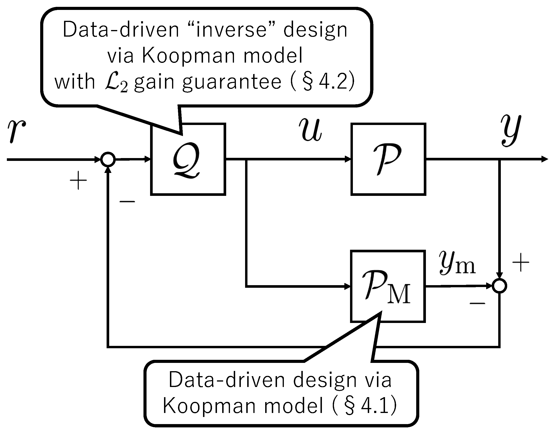
4. Result 2: Gain-Preserving Approximation of the Koopman Operator for Data-Driven Robust Controller Design

In this section, a data-driven feedback controller design is addressed based on ${\mathcal{L}}_2$ gain-preserving modeling, presented in Section 3. In particular, the data-driven IMC design is presented. The structure of the overall control system including plant system $\mathcal{P}$ and IMC is illustrated in Figure 4. IMC is composed of plant model ${\mathcal{P}}_{\mathrm{M}}$ and filter $\mathcal{Q}$, which were designed using the operating data on plant system $\mathcal{P}$, which is denoted by $\{u,y\}$, as mentioned in the figure.

Figure 4. IMC-based control system and organization of Section 4.

The procedure of the IMC design is stated as follows. Firstly, the data-driven modeling of plant $\mathcal{P}$ is addressed to construct Koopman model ${\mathcal{P}}_{\mathrm{M}}$ based on data $\{u,y\}$. This “forward” modeling is stated in Section 4.1. Secondly, the data-driven modeling of “inverse” plant ${\mathcal{P}}^{-1}$ is addressed to construct the Koopman model $\mathcal{Q}$ based on the “flipped” data $\{y,u\}$. This "backward" modeling is stated in Section 4.2.

4.1. Data-Driven Modeling of Plant System

In this subsection, the data-driven modeling of plant system $\mathcal{P}$ is addressed. Consider a discrete-time nonlinear plant system described by

$$\begin{array}{c}\hfill \mathcal{P}:\left\{\begin{array}{cc}\hfill x(k+1)& =f_{\mathrm{p}}\left(x\left(k\right),u\left(k\right)\right),\hfill \\ \hfill y\left(k\right)& =g_{\mathrm{p}}\left(x\left(k\right)\right),\hfill \end{array}\right.\end{array}$$

(19)

where $u\in {\mathbb{R}}^m$ is the input, $x\in {\mathbb{R}}^n$ is the state, $y\in {\mathbb{R}}^l$ is the output, and $f_{\mathrm{p}}(·):{\mathbb{R}}^{n+m}\to {\mathbb{R}}^n$ and $g_{\mathrm{p}}(·):{\mathbb{R}}^n\to {\mathbb{R}}^l$ are the nonlinear functions.

Data-driven modeling of $\mathcal{P}$ is used to obtain plant Koopman model ${\mathcal{P}}_{\mathrm{M}}$ described by

$$\begin{array}{c}\hfill {\mathcal{P}}_{\mathrm{M}}:\left\{\begin{array}{cc}\hfill {\psi }_{\mathrm{m}}(k+1)& =A_{\mathrm{m}}{\psi }_{\mathrm{m}}\left(k\right)+B_{\mathrm{m}}u\left(k\right),\hfill \\ \hfill y_{\mathrm{m}}\left(k\right)& =C_{\mathrm{m}}{\psi }_{\mathrm{m}}\left(k\right),\hfill \end{array}\right.\end{array}$$

(20)

where $y_{\mathrm{m}}\in {\mathbb{R}}^l$ is the output of plant model ${\mathcal{P}}_{\mathrm{M}}$ and ${\psi }_{\mathrm{m}}\left(k\right)\in {\mathbb{R}}^{N_{\mathrm{m}}}$ is the $N_{\mathrm{m}}$-dimensional lifted state given by

$$\begin{array}{c}\hfill {\psi }_{\mathrm{m}}\left(k\right):={\psi }_{\mathrm{m}}\left(x\left(k\right)\right):=\left[\begin{array}{c}{\psi }_{\mathrm{m},1}\left(x\left(k\right)\right)\\ ⋮\\ {\psi }_{\mathrm{m},N}\left(x\left(k\right)\right)\end{array}\right]\in {\mathbb{R}}^{N_{\mathrm{m}}}.\end{array}$$

For simplicity of discussion, it is assumed that

$$\begin{array}{c}\hfill {\psi }_{\mathrm{m}}\left(0\right)=0\end{array}$$

holds, i.e., the origin is the equilibrium of the zero input system.

We define the following data matrices based on the sequences of the input, output, and state of plant (19):

$$\begin{array}{cc}\hfill U_k& :=\left[u\left(k\right)u(k+1)\cdots u(k+M-1)\right]\in {\mathbb{R}}^{m\times M},\hfill \\ \hfill Y_k& :=\left[y\left(k\right)y(k+1)\cdots y(k+M-1)\right]\in {\mathbb{R}}^{l\times M},\hfill \\ \hfill {\Psi }_{\mathrm{m},k}& :=\left[{\psi }_{\mathrm{m}}\left(k\right){\psi }_{\mathrm{m}}(k+1)\cdots {\psi }_{\mathrm{m}}(k+M-1)\right]\in {\mathbb{R}}^{N_{\mathrm{m}}\times M},\hfill \\ \hfill {\Psi }_{\mathrm{m},k+1}& :=\left[{\psi }_{\mathrm{m}}(k+1){\psi }_{\mathrm{m}}(k+2)\cdots {\psi }_{\mathrm{m}}(k+M)\right]\in {\mathbb{R}}^{N_{\mathrm{m}}\times M},\hfill \end{array}$$

We assume that data matrices $\left(U_k,Y_k,{\Psi }_{\mathrm{m},k},{\Psi }_{\mathrm{m},k+1}\right)$ are available for data-driven plant modeling. The problem of data-driven modeling to construct a plant Koopman model (20) is formulated as follows.

Problem 5.

Given data matrices $(U_k,Y_k,{\Psi }_{\mathrm{m},k},{\Psi }_{\mathrm{m},k+1})$, we solve following the optimization problem:

$$\begin{array}{c}\hfill \underset{A_{\mathrm{m}},B_{\mathrm{m}},C_{\mathrm{m}}}{min}{J}_{\mathrm{m}}(A_{\mathrm{m}},B_{\mathrm{m}},C_{\mathrm{m}}),\end{array}$$

where $J_{\mathrm{m}}(A_{\mathrm{m}},B_{\mathrm{m}},C_{\mathrm{m}})$ is given by

$$\begin{array}{c}\hfill J_{\mathrm{m}}(A_{\mathrm{m}},B_{\mathrm{m}},C_{\mathrm{m}})={∥\left[\begin{array}{c}{\Psi }_{\mathrm{m},k+1}\\ Y_k\end{array}\right]-\left[\begin{array}{cc}{A}_{\mathrm{m}}& B_{\mathrm{m}}\\ C_{\mathrm{m}}& 0\end{array}\right]\left[\begin{array}{c}{\Psi }_{\mathrm{m},k}\\ U_k\end{array}\right]∥}_F^2.\end{array}$$

The solution to Problem 5 directly gives system matrices $\left(A_{\mathrm{m}},B_{\mathrm{m}},C_{\mathrm{m}}\right)$ of plant model ${\mathcal{P}}_{\mathrm{M}}$.

4.2. Data-Driven IMC with ${\mathcal{L}}_2$ Gain Guarantee

In this subsection, the data-driven modeling of filter $\mathcal{Q}$ is addressed and a data-driven IMC is designed. As stated in Remark 1, an optimal $\mathcal{Q}$ is given by inverse plant model ${\mathcal{P}}_{\mathrm{M}}$, namely, $\mathcal{Q}={\mathcal{P}}_{\mathrm{M}}^{-1}$. Aiming to find a proper and stable $\mathcal{Q}$, data-driven “inverse” modeling is addressed: $\mathcal{Q}\approx {\mathcal{P}}_{\mathrm{M}}^{-1}$ is found based on $(U_k,Y_k)$, which is the same dataset utilized for plant modeling in Section 4.1. In other words, given dataset $(U_k,Y_k)$, plant model ${\mathcal{P}}_{\mathrm{M}}$ and filter $\mathcal{Q}$ are simultaneously designed to constitute IMC.

The model of filter $\mathcal{Q}$ is given by

$$\begin{array}{c}\hfill \mathcal{Q}:\left\{\begin{array}{cc}\hfill {\psi }_{\mathrm{q}}(k+1)& =A_{\mathrm{q}}{\psi }_{\mathrm{q}}\left(k\right)+B_{\mathrm{q}}\left(r\left(k\right)-\{y\left(k\right)-y_{\mathrm{m}}\left(k\right)\}\right),\hfill \\ \hfill u\left(k\right)& =C_{\mathrm{q}}{\psi }_{\mathrm{q}}\left(k\right),\hfill \end{array}\right.\end{array}$$

(21)

where ${\psi }_{\mathrm{q}}\left(k\right)\in {\mathbb{R}}^{N_{\mathrm{q}}}$ is the $N_{\mathrm{q}}$-dimensional lifted state given by

$$\begin{array}{c}\hfill {\psi }_{\mathrm{q}}\left(k\right):={\psi }_{\mathrm{q}}\left(u\left(k\right)\right):=\left[\begin{array}{c}u\left(k\right)\\ {\psi }_{\mathrm{q},1}\left(u\left(k\right)\right)\\ ⋮\\ {\psi }_{\mathrm{q},N-1}\left(u\left(k\right)\right)\end{array}\right]\in {\mathbb{R}}^{N_{\mathrm{q}}},\end{array}$$

and $A_{\mathrm{q}}$, $B_{\mathrm{q}}$, and $C_{\mathrm{q}}$ are the constant matrices. In addition, it is assumed that ${\psi }_{\mathrm{q}}\left(0\right)=0$ holds. Due to the definition of ${\psi }_{\mathrm{q}}\left(u\left(k\right)\right)$, $C_{\mathrm{q}}$ must be

$$\begin{array}{c}\hfill C_{\mathrm{q}}=\left[\begin{array}{cccc}I& 0& \cdots & 0\end{array}\right].\end{array}$$

As stated in Proposition 1, a requirement imposed on $\mathcal{Q}$ is its ${\mathcal{L}}_2$ stability. In addition, noting that modeling errors in ${\mathcal{P}}_{\mathrm{M}}$, given in Section 4.1, inevitably exist, $\mathcal{Q}$ must be robust against the modeling error. In the following discussion, assume that the error in plant model ${\mathcal{P}}_{\mathrm{M}}$ is characterized by the ${\mathcal{L}}_2$ gain such that $\parallel \mathcal{P}-{\mathcal{P}}_{\mathrm{M}}{\parallel }_{{\mathcal{L}}_2}\le {\gamma }_{\mathrm{p}}$ for some ${\gamma }_{\mathrm{p}}$. Then, the ${\mathcal{L}}_2$ gain-preserving model, given in Section 3, is applied to the design of $\mathcal{Q}$ such that $\mathcal{Q}$ is ${\mathcal{L}}_2$ stable and ${\parallel \mathcal{Q}\parallel }_{{\mathcal{L}}_2}\le 1/{\gamma }_{\mathrm{p}}$ holds.

For simplicity of notation, we further define the data matrices based on $U_k$

$$\begin{array}{cc}\hfill {\Psi }_{\mathrm{q},k}& :=\left[{\psi }_{\mathrm{q}}\left(k\right)\cdots {\psi }_{\mathrm{q}}(k+M-1)\right]\in {\mathbb{R}}^{N_{\mathrm{q}}\times M},\hfill \\ \hfill {\Psi }_{\mathrm{q},k+1}& :=\left[{\psi }_{\mathrm{q}}(k+1)\cdots {\psi }_{\mathrm{q}}(k+M)\right]\in {\mathbb{R}}^{N_{\mathrm{q}}\times M}.\hfill \end{array}$$

The problem of data-driven modeling to construct filter (21) where a ${\mathcal{L}}_2$ gain specification is imposed as ${\parallel \mathcal{Q}\parallel }_{{\mathcal{L}}_2}\le {\gamma }_{\mathrm{q}}$ is formulated as follows.

Problem 6.

Given a positive constant ${\gamma }_{\mathrm{q}}$ and data matrices $\left(Y_k,{\Psi }_{\mathrm{q},k},{\Psi }_{\mathrm{q},k+1}\right)$, we solve the following optimization problem:

$$\begin{array}{cccc}\hfill & \underset{P_{\mathrm{q}},A_{\mathrm{q}},B_{\mathrm{q}}}{min}\hfill & \hfill & J_{\mathrm{q}}(A_{\mathrm{q}},B_{\mathrm{q}})\hfill \\ \hfill & subto\hfill & \hfill & P_{\mathrm{q}}\succ 0\hfill \\ \hfill & \hfill & \hfill & {\left[\begin{array}{cc}{A}_{\mathrm{q}}& B_{\mathrm{q}}\\ I& 0\end{array}\right]}^{\top }\left[\begin{array}{cc}{P}_{\mathrm{q}}& 0\\ 0& -P_{\mathrm{q}}\end{array}\right]\left[\begin{array}{cc}{A}_{\mathrm{q}}& B_{\mathrm{q}}\\ I& 0\end{array}\right]+\left[\begin{array}{cc}{C}_{\mathrm{q}}^{\top }{C}_{\mathrm{q}}& 0\\ 0& -{\gamma }_{\mathrm{q}}^{2}I\end{array}\right]\prec 0,\hfill \end{array}$$

(22)

where

$$\begin{array}{c}\hfill J_{\mathrm{q}}(A_{\mathrm{q}},B_{\mathrm{q}}):={∥{\Psi }_{\mathrm{q},k+1}-\left[A_{\mathrm{q}}{B}_{\mathrm{q}}\right]\left[\begin{array}{c}{\Psi }_{\mathrm{q},k}\\ Y_k\end{array}\right]∥}_F^2.\end{array}$$

(23)

The solution to Problem 6 gives system matrices $\left(A_{\mathrm{q}},B_{\mathrm{q}},C_{\mathrm{q}}\right)$ for filter $\mathcal{Q}$, and ${\parallel \mathcal{Q}\parallel }_{{\mathcal{L}}_2}\le {\gamma }_{\mathrm{q}}$ holds. Note that Problem 6 is in the class of non-convex optimization and is numerically intractable. In the same manner as the study in Section 3, a computationally efficient algorithm is applicable to the problem.

In summary, the overall controller is constructed based on the solutions to Problems 5 and 6. The following proposition states the robust stability of the overall control system.

Proposition 6.

Suppose that $\parallel \mathcal{P}-{\mathcal{P}}_{\mathrm{M}}{\parallel }_{{\mathcal{L}}_2}\le {\gamma }_{\mathrm{p}}$ holds, and consider that filter $\mathcal{Q}$ is designed by the solution to Problem 6. Then, the IMC-based control system, illustrated in Figure 4, is ${\mathcal{L}}_2$ stable if ${\gamma }_{\mathrm{p}}{\gamma }_{\mathrm{q}}<1$ holds.

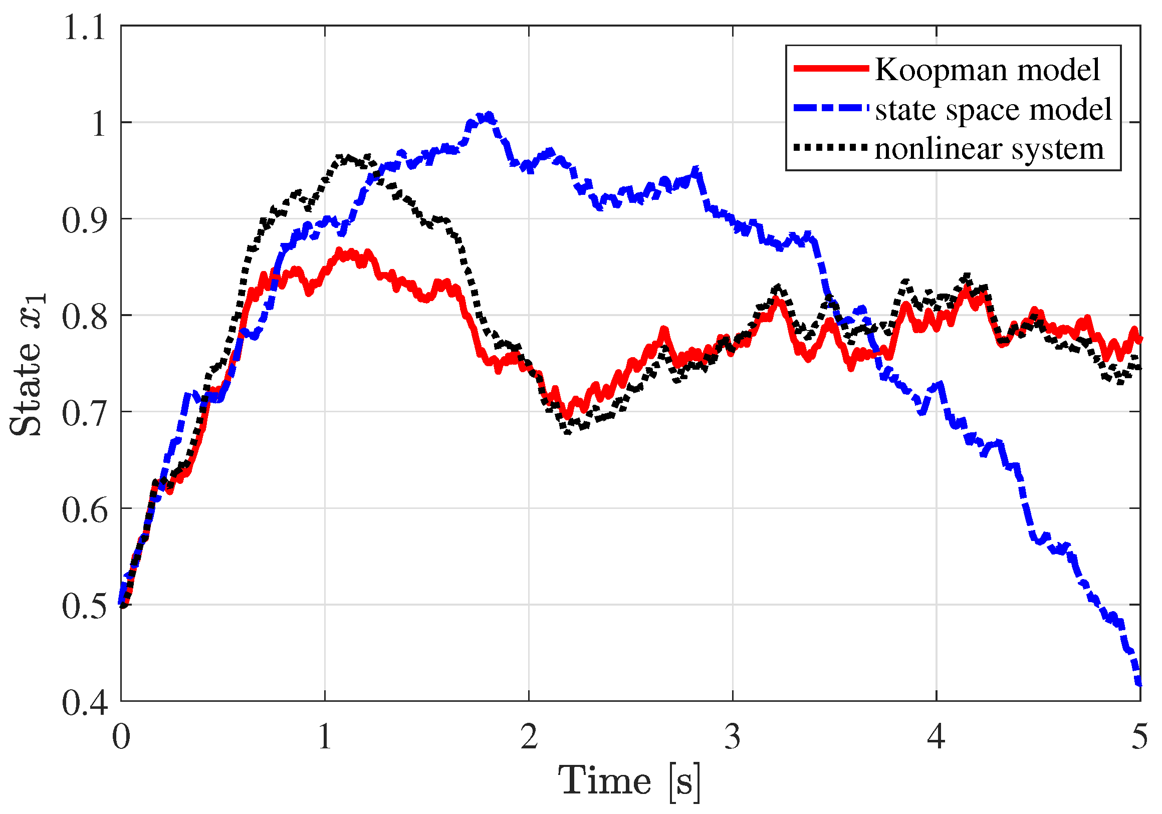
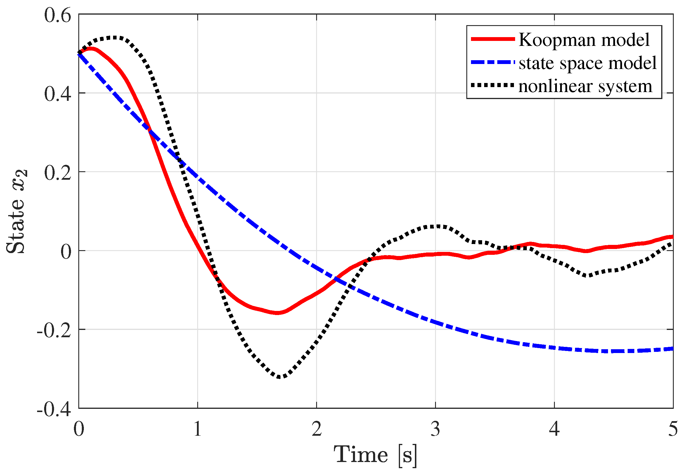
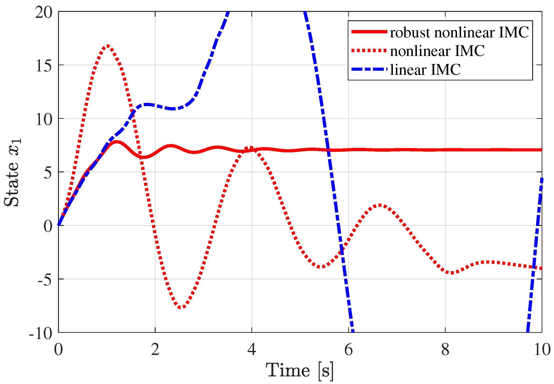
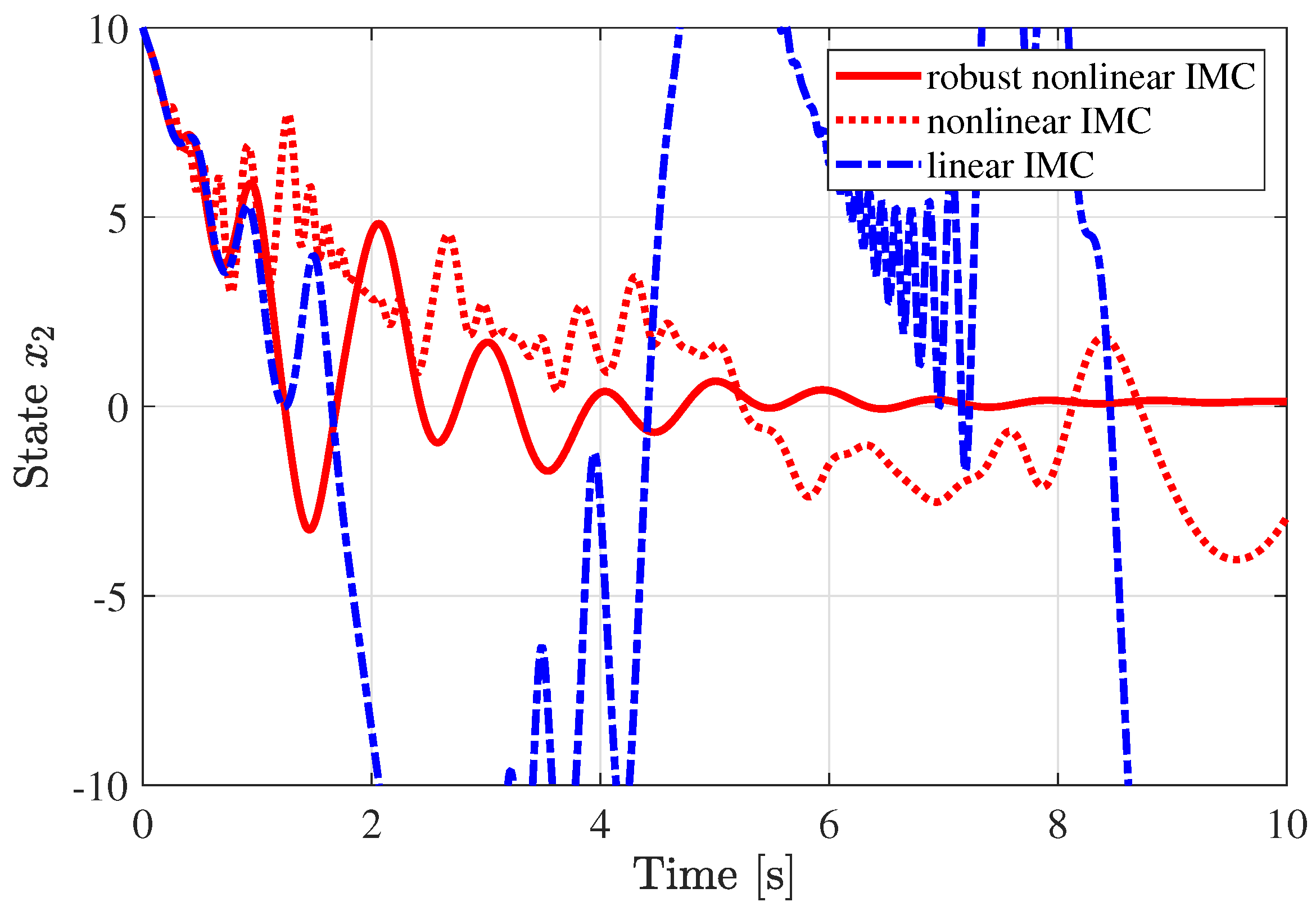
5. Numerical Experiment

In this section, we demonstrate the procedure for designing a data-driven robust IMC. Let us consider a plant system described by the nonlinear state-space equation:

$$\begin{array}{c}\hfill \mathcal{P}:\left\{\begin{array}{ccc}{\dot{x}}_1\left(t\right)& =& x_2\left(t\right)+u\left(t\right),\hfill \\ {\dot{x}}_2\left(t\right)& =& -2x_2\left(t\right)+3x_1\left(t\right)cos\left(2x_1\left(t\right)\right),\hfill \\ y\left(t\right)& =& x_2\left(t\right).\hfill \end{array}\right.\end{array}$$

(24)

System (24) possesses stable equilibria such as $(x_1,x_2,u)=(\frac{1}{4}\pi +\pi s,0,0)$ for some integar s. In this demonstration, we design a feedback controller to further improve the output regulation performance. To this end, the data-driven IMC is constructed by the following stages. (1) Data-driven modeling of plant system (24) is addressed to construct a plant Koopman model ${\mathcal{P}}_{\mathrm{M}}$. The details of this stage are given in Section 4.1. (2) Data-driven modeling of the inverse plant system is addressed to construct filter $\mathcal{Q}$. In filter construction, aiming to guarantee the stability of the control system, ${\mathcal{L}}_2$ gain-preserving modeling is applied to $\mathcal{Q}$. The details of the modeling method are stated in Section 4.2.

At Stage 1, the time series of $x\left(t\right)$, $u\left(t\right)$, and $y\left(t\right)$ are sampled at each 0.01 time period from plant system (24), which are denoted by $\left\{x\right(k\left)\right\}$, $\left\{u\right(k\left)\right\}$, and $\left\{y\right(k\left)\right\}$, respectively. Input series $\left\{u\right(k\left)\right\}$ is the sine wave given by $csin\left(0.02\pi k\right)$, and amplitude c is randomly chosen from $\{0.1,0.2,\cdots ,5\}$. Then, its corresponding state and output series $\left\{x\right(k\left)\right\}$ and $\left\{y\right(k\left)\right\}$ are measured and collected. In total, the data of 50,000 samples are obtained. Note that the computational cost for the data-driven modeling presented in this paper does not largely depend on data volume, but it strongly depends on the dimension of the lifted state-space, determined by the users.

Let lifting function ${\psi }_m\left(x\left(k\right)\right)$ be composed of state $x\left(k\right)={[x_1\left(k\right),x_2\left(k\right)]}^{\top }$ and thin plate spline radial basis functions ${\psi }_{m,i}\left(x\left(k\right)\right)$, $i\in \{1,2,\dots ,8\}$, described by

$$\begin{array}{c}\hfill {\psi }_{m,i}\left(x\left(k\right)\right)={\parallel x\left(k\right)-r_{m,i}\parallel }_2^{2}ln\parallel x\left(k\right)-r_{m,i}{\parallel }_2,\end{array}$$

where the values of $r_{m,i}$ are selected randomly from the uniform distribution on the unit box. In other words, lifting function ${\psi }_m\left(x\left(k\right)\right)$ is given by

$$\begin{array}{c}\hfill {\psi }_m\left(x\left(k\right)\right)={\left[x\left(k\right){\psi }_{m,1}\left(x\left(k\right)\right)\cdots {\psi }_{m,8}\left(x\left(k\right)\right)\right]}^{\top }\in {\mathbb{R}}^{2+8}.\end{array}$$

By applying the data-driven modeling presented in Section 4.1 to the data, we obtain plant Koopman model ${\mathcal{P}}_{\mathrm{M}}$. The coefficient matrices of constucted ${\mathcal{P}}_{\mathrm{M}}$ are given as follows.

$$\begin{array}{cc}\hfill A_{\mathrm{m}}& =\left[\begin{array}{cccccccccc}1.00& 0.01& 0& 0& 0& 0& 0& 0& 0& 0\\ 0.07& 0.98& 0& 0.04& -0.02& -0.13& 0.02& 0.01& 0.02& 0.08\\ 0.10& -0.07& 1.00& 0.06& -0.01& -0.25& -0.05& 0& 0.05& 0.16\\ -0.14& 0.08& 0& 0.96& 0.03& 0.05& 0& 0.03& -0.06& -0.02\\ 0.12& -0.07& 0& 0.07& 0.98& -0.27& -0.04& 0& 0.05& 0.19\\ -0.08& 0.04& 0.01& -0.01& 0.02& 0.94& 0.01& 0.02& -0.04& 0.05\\ 0.06& -0.08& 0.02& 0.03& -0.03& -0.09& 0.96& -0.03& 0.03& 0.08\\ -0.17& 0.09& 0.01& -0.03& 0.04& -0.05& -0.01& 1.03& -0.08& 0.07\\ 0.04& 0.02& 0.01& 0.11& -0.04& -0.41& 0.01& 0.03& 0.99& 0.29\\ -0.05& 0.01& 0.01& -0.01& 0.01& -0.06& 0& 0.01& -0.02& 1.05\end{array}\right],\hfill \\ \hfill B_{\mathrm{m}}& ={\left[\begin{array}{cccccccccc}0.01& 0& 0.02& 0.01& 0.01& 0.02& 0& 0.03& -0.01& 0.02\end{array}\right]}^{\top },\hfill \\ \hfill C_{\mathrm{m}}& =\left[\begin{array}{cccccccccc}0& 1.00& 0& 0& 0& 0& 0& 0& 0& 0\end{array}\right].\hfill \end{array}$$

For a comparative study, a linear state-space model is constructed, where the lifting function of ${\mathcal{P}}_{\mathrm{M}}$ is replaced by $x\left(t\right)$.

The modeling result is illustrated in Figure 5 and Figure 6, where the state response with respect to the Gaussian noise input is shown. The state response for Koopman model ${\mathcal{P}}_{\mathrm{M}}$, linear state space model, and plant system $\mathcal{P}$ are depicted by the red, solid; blue, dashed; and black, dotted lines, respectively. We see that the plant Koopman model ${\mathcal{P}}_{\mathrm{M}}$ accurately expresses the nonlinear behavior generated by complex system (24), while the linear model cannot.

Figure 5. State $x_1$ of the Koopman model, the linear state-space model, and the plant system.

Figure 6. State $x_2$ of the Koopman model, the linear state-space model, and the plant system.

At Stage 2, based on flipped input–output data $\left\{y\right(k),u(k\left)\right\}$, we design filter $\mathcal{Q}$ such that any desired ${\mathcal{L}}_2$ gain specification is satisfied. In the same manner as the plant modeling, let lifting function ${\psi }_q\left(u\left(k\right)\right)$ be composed of input $u\left(k\right)$ and thin plate spline radial basis functions ${\psi }_{q,i}\left(u\left(k\right)\right)$, $i\in \{1,2,\dots ,4\}$, where ${\psi }_{q,i}\left(u\left(k\right)\right)$ is given by

$$\begin{array}{c}\hfill {\psi }_{q,i}\left(u\left(k\right)\right)={\parallel u\left(k\right)-r_{q,i}\parallel }_2^{2}ln\parallel u\left(k\right)-r_{q,i}{\parallel }_2\end{array}$$

and the values of $r_{q,i}$ are selected randomly from the uniform distribution in the unit box. Then, lifting function ${\psi }_q\left(u\left(k\right)\right)$ is described by

$$\begin{array}{c}\hfill {\psi }_q\left(u\left(k\right)\right)={\left[u\left(k\right){\psi }_{q,1}\left(u\left(k\right)\right)\cdots {\psi }_{q,4}\left(u\left(k\right)\right)\right]}^{\top }\in {\mathbb{R}}^{1+4}.\end{array}$$

(25)

${\mathcal{L}}_2$ gain-preserving inverse modeling is applied to design filter $\mathcal{Q}$. As implied in Section 4.2, the modeling method requires us to assume the modeling error in ${\mathcal{P}}_{\mathrm{M}}$ such that $\parallel \mathcal{P}-{\mathcal{P}}_{\mathrm{M}}{\parallel }_{{\mathcal{L}}_2}\le {\gamma }_{\mathrm{p}}$ and to impose the ${\mathcal{L}}_2$ gain constraint on $\mathcal{Q}$ such that ${\parallel \mathcal{Q}\parallel }_{{\mathcal{L}}_2}\le {\gamma }_{\mathrm{q}}$ with ${\gamma }_{\mathrm{q}}=1/{\gamma }_{\mathrm{p}}$. In general, it is difficult to estimate ${\gamma }_{\mathrm{p}}$, and we cannot determine ${\gamma }_{\mathrm{q}}$ in a systematic manner. In practice, ${\gamma }_{\mathrm{q}}$ is a tunable parameter, determined by the users depending on their design aims. A small value of ${\gamma }_{\mathrm{q}}$, which imposes a severe constraint on $\mathcal{Q}$, improves the robustness and stability margin for the controlled system, while a large value tends to improve the nominal control performance. In this demonstration, we set ${\gamma }_{\mathrm{p}}=0.5$ to priorize robustness.

The modeling problem was solved in a computationally efficient manner by using YALMIP [37] and SeDuMi [38] to construct filter $\mathcal{Q}$. For example, it took 12.26 s to solve the LMIs in Problem 3 with a laptop (CPU: Core i7-8665U 1.90 GHz). The coefficient matrices of constructed $\mathcal{Q}$ are given as follows.

$$\begin{array}{cc}\hfill A_{\mathrm{q}}& =\left[\begin{array}{ccccc}0.45& 0.04& 0.01& 0& -0.05\\ -1.07& 0.94& 0.10& -0.05& -0.03\\ -0.71& 0.08& 0.91& -0.04& 0.02\\ 0.19& 0.24& -0.34& 0.95& 0.11\\ 1.59& -0.14& -0.01& -0.02& 1.14\end{array}\right],\hfill \\ \hfill B_{\mathrm{q}}& ={\left[\begin{array}{ccccc}0& 1.34& 1.43& 1.55& 1.34\end{array}\right]}^{\top },\hfill \\ \hfill C_{\mathrm{q}}& =\left[\begin{array}{ccccc}1.00& 0& 0& 0& 0\end{array}\right].\hfill \end{array}$$

Then, ${\mathcal{P}}_{\mathrm{M}}$ and $\mathcal{Q}$ constitute a nonlinear IMC, the structure of which is illustrated in Figure 4.

For a comparative study, another filter $\mathcal{Q}$ is designed with no ${\mathcal{L}}_2$ gain constraint, and its corresponding nonlinear IMC is constructed. The controller with unconstrained $\mathcal{Q}$ can have high gain, which tends to improve the nominal control performance while deteriorating the robustness. In addition, a data-driven linear IMC is constructed with no ${\mathcal{L}}_2$ gain constraint, where the lifting functions of ${\mathcal{P}}_{\mathrm{M}}$ and $\mathcal{Q}$ are replaced by $x\left(t\right)$ and $u\left(t\right)$, respectively.

The simulation of regulation control achieved by the controllers is illustrated in Figure 7 and Figure 8. In the figures, the state trajectory achieved by the proposed constrained nonlinear IMC, unconstrained nonlinear IMC, and unconstrained linear IMC are drawn by the red, solid; red, dotted; and blue, dashed lines, respectively. We see that the proposed constrained IMC robustly achieves output regulation, i.e., $x_2\left(t\right)$ converges to the origin under the presence of the modeling error, while the others cannot. This concludes that the proposed gain-constrained IMC contributes to robust stability for the control system.

Figure 7. Controlled state $x_1$ achieved by the proposed IMC, the nonlinear IMC, and the linear IMC.

Figure 8. Controlled state $x_2$ achieved by the proposed IMC, the nonlinear IMC, and the linear IMC.

6. Conclusions

This paper addressed data-driven modeling of a nonlinear dynamical system, described by the Koopman operator while incorporating a priori known information about the ${\mathcal{L}}_2$ gain. Then, a ${\mathcal{L}}_2$ gain-preserving data-driven model was formulated, and its LMI-based solution method was presented. The modeling method was applied to the design of a data-driven robust nonlinear IMC, and its design demonstration was presented.

The presented data-driven IMC can be a fundamental control technique and can be extended in various directions. These directions include pursuing ${\mathcal{H}}_2$/${\mathcal{H}}_{\infty }$ control performance and adaptating it for filter $\mathcal{Q}$.

References

- Kutz, J.N.; Brunton, S.L.; Brunton, B.W.; Proctor, J.L. Dynamic Mode Decomposition: Data-Driven Modeling of Complex Systems; SIAM: Philadelphia, PA, USA, 2016. [Google Scholar]
- Ljung, L.; Andersson, C.; Tiels, K.; Schön, T.B. Deep learning and system identification. In Proceedings of the IFAC World Congress 2020, Berlin, Germany, 12–17 July 2020. [Google Scholar]
- Lacy, S.L.; Bernstein, D.S. Subspace identification with guaranteed stability using constrained optimization. IEEE Trans. Autom. Control 2003, 48, 1259–1263. [Google Scholar] [CrossRef]
- Okada, M.; Sugie, T. Subspace system identification considering both noise attenuation and use of prior knowledge. In Proceedings of the 35th IEEE Conference on Decision and Control, Kobe, Japan, 11–13 December 1996; pp. 3662–3667. [Google Scholar]
- Miller, D.N.; De Callafon, R.A. Subspace identification with eigenvalue constraints. Automatica 2013, 49, 2468–2473. [Google Scholar] [CrossRef]
- Alenany, A.; Shang, H.; Soliman, M.; Ziedan, I. Improved subspace identification with prior information using constrained least squares. IET Control Theory Appl. 2011, 5, 1568–1576. [Google Scholar] [CrossRef]
- Yoshimura, S.; Matsubayashi, A.; Inoue, M. System identification method inheriting steady-state characteristics of existing model. Int. J. Control 2019, 92, 2701–2711. [Google Scholar] [CrossRef]
- Goethals, I.; Van Gestel, T.; Suykens, J.; Van Dooren, P.; De Moor, B. Identification of positive real models in subspace identification by using regularization. IEEE Trans. Autom. Control 2003, 48, 1843–1847. [Google Scholar] [CrossRef]
- Hoagg, J.B.; Lacy, S.L.; Erwin, R.S.; Bernstein, D.S. First-order-hold sampling of positive real systems and subspace identification of positive real models. In Proceedings of the 2004 American Control Conference, Boston, MA, USA, 30 June–2 July 2004; pp. 861–866. [Google Scholar]
- Abe, Y.; Inoue, M.; Adachi, S. Subspace identification method incorporated with a priori information characterized in frequency domain. In Proceedings of the 2016 European Control Conference, Aalborg, Denmark, 29 June–1 July 2016; pp. 1377–1382. [Google Scholar]
- Inoue, M. Subspace identification with moment matching. Automatica 2019, 99, 22–32. [Google Scholar] [CrossRef]
- Zhou, K.; Doyle, J.C.; Glover, K. Robust and Optimal Control; Prentice Hall: Hoboken, NJ, USA, 1996. [Google Scholar]
- Brunton, S.L.; Brunton, B.W.; Proctor, J.L.; Kutz, J.N. Koopman invariant subspaces and finite linear representations of nonlinear dynamical systems for control. PLoS ONE 2016, 11, e0150171. [Google Scholar]
- Kaiser, E.; Kutz, J.N.; Brunton, S.L. Data-driven discovery of Koopman eigenfunctions for control. arXiv 2017, arXiv:1707.01146. [Google Scholar]
- Hara, K.; Inoue, M.; Sebe, N. Learning Koopman operator under dissipativity constraints. In Proceedings of the IFAC World Congress 2020, Berlin, Germany, 12–17 July 2020. [Google Scholar]
- Korda, M.; Mezić, I. Linear predictors for nonlinear dynamical systems: Koopman operator meets model predictive control. Automatica 2018, 93, 149–160. [Google Scholar] [CrossRef]
- Narasingam, A.; Kwon, J.S.I. Koopman Lyapunov-based model predictive control of nonlinear chemical process systems. AIChE J. 2019, 65, e16743. [Google Scholar] [CrossRef]
- Ma, X.; Huang, B.; Vaidya, U. Optimal quadratic regulation of nonlinear system using Koopman operator. In Proceedings of the 2019 American Control Conference, Philadelphia, PA, USA, 10–12 July 2019; pp. 4911–4916. [Google Scholar]
- Broad, A.; Abraham, I.; Murphey, T.; Argall, B. Data-driven Koopman operators for model-based shared control of human–machine systems. Int. J. Robot. Res. 2020, 39, 1178–1195. [Google Scholar] [CrossRef]
- Peitz, S.; Otto, S.E.; Rowley, C.W. Data-driven model predictive control using interpolated Koopman generators. SIAM J. Appl. Dyn. Syst. 2020, 19, 2162–2193. [Google Scholar] [CrossRef]
- Choi, H.; Vaidya, U.; Chen, Y. A convex data-driven approach for nonlinear control synthesis. arXiv 2020, arXiv:2006.15477. [Google Scholar]
- Uchida, D.; Yamashita, A.; Asama, H. Data-driven Koopman controller synthesis based on the extended H2 norm characterization. IEEE Control Syst. Lett. 2021, 5, 1795–1800. [Google Scholar] [CrossRef]
- Lian, Y.; Wang, R.; Jones, C.N. Koopman based data-driven predictive control. arXiv 2021, arXiv:2102.05122. [Google Scholar]
- Otto, S.E.; Rowley, C.W. Koopman operators for estimation and control of dynamical systems. Annu. Rev. Control Robot. Auton. Syst. 2021, 4. [Google Scholar] [CrossRef]
- Bevanda, P.; Sosnowski, S.; Hirche, S. Koopman operator dynamical models: Learning, analysis and control. arXiv 2021, arXiv:2102.02522. [Google Scholar]
- Mauroy, A.; Susuki, Y.; Mezić, I. The Koopman Operator in Systems and Control; Springer: Berlin, Germany, 2020. [Google Scholar]
- Sebe, N. Sequential convex overbounding approximation method for bilinear matrix inequality problems. IFAC-PapersOnLine 2018, 51, 102–109. [Google Scholar] [CrossRef]
- Garcia, C.E.; Morari, M. Internal model control. A unifying review and some new results. Ind. Eng. Chem. Process. Des. Dev. 1982, 21, 308–323. [Google Scholar] [CrossRef]
- Economou, C.G.; Morari, M.; Palsson, B.O. Internal model control: Extension to nonlinear system. Ind. Eng. Chem. Process. Des. Dev. 1986, 25, 403–411. [Google Scholar] [CrossRef]
- Nguyen, H.T.; Kaneko, O.; Yamamoto, S. Data-driven IMC for non-minimum phase systems-Laguerre expansion approach. In Proceedings of the 50th IEEE Conference on Decision and Control and 2011 European Control Conference, Orlando, FL, USA, 12–15 December 2011; pp. 476–481. [Google Scholar]
- Nguyen, H.T.; Kaneko, O.; Wadagaki, Y.; Yamamoto, S. Fictitious reference iterative tuning of internal model controllers for non-minimum phase plants. In Proceedings of the SICE Annual Conference 2011, Tokyo, Japan, 13–18 September 2011; pp. 2608–2613. [Google Scholar]
- Rojas, J.; Vilanova, R. Data-driven based IMC control. Int. J. Innov. Comput. Inf. Control 2012, 8, 1557–1574. [Google Scholar]
- Rueda-Escobedo, J.G.; Schiffer, J. Data-driven internal model control of second-order discrete Volterra systems. In Proceedings of the 59th IEEE Conference on Decision and Control, Jeju, Korea, 14–18 December 2020; pp. 4572–4579. [Google Scholar]
- Desoer, C.A.; Vidyasagar, M. Feedback Systems: Input-Output Properties; SIAM: Philadelphia, PA, USA, 1975. [Google Scholar]
- Brogliato, B.; Lozano, R.; Maschke, B.; Egeland, O. Dissipative Systems Analysis and Control: Theory and Applications; Springer: Berlin, Germany, 2007. [Google Scholar]
- Saxena, S.; Hote, Y.V. Advances in internal model control technique: A review and future prospects. IETE Tech. Rev. 2012, 29, 461–472. [Google Scholar] [CrossRef]
- Lofberg, J. YALMIP: A toolbox for modeling and optimization in MATLAB. In Proceedings of the 2004 IEEE International Conference on Robotics and Automation, Taipei, Taiwan, 2–4 September 2004; pp. 284–289. [Google Scholar]
- Sturm, J.F. Using SeDuMi 1.02, a MATLAB toolbox for optimization over symmetric cones. Optim. Methods Softw. 1999, 11, 625–653. [Google Scholar] [CrossRef]
Publisher’s Note: MDPI stays neutral with regard to jurisdictional claims in published maps and institutional affiliations. |
© 2021 by the authors. Licensee MDPI, Basel, Switzerland. This article is an open access article distributed under the terms and conditions of the Creative Commons Attribution (CC BY) license (https://creativecommons.org/licenses/by/4.0/).