A New Compromise Design Plan for Accelerated Failure Time Models with Temperature as an Acceleration Factor

Abstract

An accelerated life test of a product or material consists of the observation of its failure time when it is subjected to conditions that stress the usual ones. The purpose is to obtain the parameters of the distribution of the time-to-failure for usual conditions through the observed failure times. A widely used method to provoke an early failure in a mechanism is to modify the temperature at which it is used. In this paper, the statistically optimal plan for Accelerated Failure Time (AFT) models, when the accelerated failure process is described making use of Arrhenius or Eyring equations, was calculated. The result was a design that had only two stress levels, as is common in other AFT models and that is not always practical. A new compromise plan was presented as an alternative to the widely used “4:2:1 plan”. The three-point mixture design proposed specified a support point in the interval that was optimal for the estimation of the parameters in AFT models, rather than simply the middle point. It was studied in comparison to different commonly used designs, and it proved to have a higher D-efficiency than the others.

1. Introduction

Accelerated testing consists of subjecting a product or material to a high stress that shortens its life or hastens the degradation of its performance. Stress can refer to different accelerating variables, such as temperature, humidity, pressure, etc. The main reasons to perform over-stress testing is to estimate the life expectancy of the product under normal conditions (at lower or null stress levels) [1], i.e., to obtain the parameters of the distribution of the time-to-failure for usual conditions through the observed failure times. Generally, there is some information available (based on physical/chemical theory or previous experience with similar tests) that can be used to explain the existing relationship between the accelerating variables and the failure mechanism and that can be used to identify a model and justify the extrapolation [2]. The Accelerated Failure Time (AFT) model provides a natural formulation of the effects of covariates on the response variable. The aim of AFT models is to study how the survival function is directly affected by the explanatory variables, rather than the hazard function in the commonly used proportional hazards models. Unlike proportional hazards models, AFT models are mostly fully parametric, which facilitates their interpretation measuring the effect of the corresponding covariate on the survival time. Estimating the failure time distribution of the long-term performance of a product or material is particularly important in the field of manufacturing to demonstrate product or material reliability [3,4,5,6], although AFT models are also used for analyzing clinical trial data [7,8,9] and genomic studies [10,11].

One of the most widely used methods to accelerate a failure mechanism is to modify the temperature at which it is used. Products and materials can be tested at temperatures above (or below) their normal use temperature so that defects or failure modes that may appear in the distant future at normal use temperatures can be detected in short times. The typical failure mode is dependent on migration/diffusion or chemical degradation (resulting in eventual weakening and failure). These types of failures are typically found in electronic components, but can also occur in other types of products or materials such as adhesives, batteries, etc. More on the effects of temperature on short-time failures can be found in [12,13,14].

As important as it is to observe failures in a short period of time to extrapolate survival time in usual conditions, it is important to optimally select the points of stress in which the observations shall be taken; that is, to select the points of stress efficiently so that they provide as much information as possible about the failure process. Meeker [15] and Meeker and Nelson [16] obtained the optimal tests that minimized the asymptotic variance of the maximum likelihood estimator of the pth percentile at design stress. Bai and Chung [17] studied optimal designs for tests in which two levels of stress were constantly applied and the failed items were replaced. In this paper, the accelerated failure process was described making use of Arrhenius and Eyring equations. AFT models are introduced in Section 2, and D-optimal designs when the acceleration factor is temperature are calculated in Section 3.

As expected, as is common in AFT models with single stress and type I censoring [18], the statistically optimal plan has only two stress levels. These optimal two-level plans are not always practical [19], and there has been extensive research on “compromise design plans” ([20,21,22,23], to name a few). Meeker [15] proposed several compromise plans and concluded that the best plan has three equally spaced test stresses, and between 10% and 20% of the samples are taken at the middle stress level, as collected in Chen et al. [18]. This developed into the so-called “4:2:1 plan”, proposed by Meeker and Hahn [24] and still widely used. A new alternative compromise plan is presented in Section 4, combining different optimal designs. A numerical example, showing the comparisons between the most commonly used designs and the proposed mixture of designs, is presented in Section 5.

1.1. Design of Experiments Background

Let T represent the response variable time-to-event, assumed to be a random variable from a parametric distribution with vector of parameters $\mathit{\theta }$. The response T is observed under certain experimental conditions represented by $\mathbf{x}$, where the vector of covariates, $\mathbf{X}$, is chosen from a compact design space $\mathcal{X}$. An approximate design, $\xi$, is a collection of n different support points, ${\mathbf{x}}_1,{\mathbf{x}}_2,\dots ,{\mathbf{x}}_n$, and weights, $\xi \left({\mathbf{x}}_1\right),\xi \left({\mathbf{x}}_2\right),\cdots ,\xi \left({\mathbf{x}}_n\right)$, defining a discrete probability on $\mathcal{X}$. The Fisher Information Matrix (FIM) captures the information given by a design $\xi$. Loosely speaking, it describes the amount of information about an unknown parameter provided by the data. The FIM is defined as:

$$M(\xi ,\mathit{\theta })=\sum _{i=1}^{n}I(\mathit{\theta };{\mathbf{x}}_i)\xi \left({\mathbf{x}}_i\right),I(\mathit{\theta };{\mathbf{x}}_i)=\mathbb{E}\left(-\frac{{\partial }^{2}LL(\mathit{\theta };t,{\mathbf{x}}_i)}{\partial \mathit{\theta }\partial {\mathit{\theta }}^{\prime }}\right),$$

(1)

where $LL(\mathit{\theta };t,{\mathbf{x}}_i)$ is the log-likelihood function for experimental conditions ${\mathbf{x}}_i$. The inverse of the FIM, $M^{-1}(\xi ,\mathit{\theta })$, for independent observations, is proportional to the asymptotic covariance matrix of the maximum likelihood estimate of $\mathit{\theta }$. Optimal designs aim to minimize the covariance matrix, i.e., maximize a function $\varphi$ of the information matrix, called the optimality criterion.

1.1.1. D-Optimal Designs

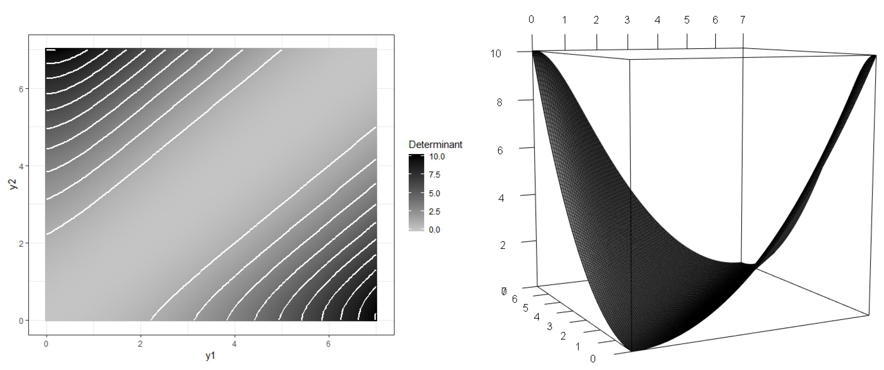
The most popular criterion is D-optimality. For non-linear models, the FIM (and thus the optimal designs) are dependent on the model parameters. Therefore, to obtain locally optimal designs’ initial (also called nominal) values, ${\mathit{\theta }}_0$ are needed. For a given ${\mathit{\theta }}_0$, D-optimality maximizes the determinant of the FIM, i.e., it minimizes the volume of the confidence ellipsoid of estimators of the parameters of the model [25].

The D-optimal design has equal weights when the number of support points is the same as the number of parameters of the model, $n_p$. From the General Equivalence Theorem (GET) [26], a design ${\xi }_D$ is D-optimal if and only if:

$$\psi ({\xi }_D,\mathit{\theta },\mathbf{x})=\mathrm{tr}\left[M^{-1}({\xi }_D,\mathit{\theta })I(\mathit{\theta };\mathbf{x})\right]\le n_p\forall \mathbf{x}\in \mathcal{X}.$$

(2)

Moreover, equality is reached at the support points of the design. $\psi ({\xi }_D,\mathit{\theta },\mathbf{x})$ is known as the sensitivity function.

Let ${\mathit{\theta }}_0$ represent the actual values of the parameters, which give an optimal design ${\xi }_D^{*}$. Then, how good a design $\xi$ is can be studied by calculating its efficiency when compared to ${\xi }_D^{*}$. The D-efficiency is computed as:

$${\mathit{Eff}}_{{\mathit{\theta }}_0}\left(\xi \right)={\left[{\displaystyle \frac{detM(\xi ,{\mathit{\theta }}_0)}{detM({\xi }_D^{*},{\mathit{\theta }}_0)}}\right]}^{\frac{1}{n_p}}.$$

(3)

If the design $\xi$ has D-efficiency p and N experiments are performed under it, the same accuracy in the estimations can be reached by performing $pN$ experiments under the optimal design ${\xi }_D^{*}$.

The efficiency function (3) can also be used to check the robustness of a design by considering different sets of values to be the true parameters and computing the efficiency of the D-optimal design with respect to the design obtained for the new set of parameters.

1.1.2. c-Optimal Designs

c-optimality aims to minimize the variance of the estimator of a linear combination of the unknown parameters $c_1{\theta }_1+c_2{\theta }_2+\dots +c_m{\theta }_m=c^T\mathit{\theta }$. c-optimal designs are commonly used when the main objective is to estimate a specific parameter, i.e., when c is chosen to be the m-dimensional euclidean vector $(0,\dots ,1_i,\dots ,0)$, the criterion leads to the best design for the estimation of the parameter ${\theta }_i$, and thus, the corresponding c-optimal design minimizes the variance of the estimator of ${\theta }_i$. This is done by minimizing the $(i,i)$ element of $M^{-1}(\xi ,\mathit{\theta })$.

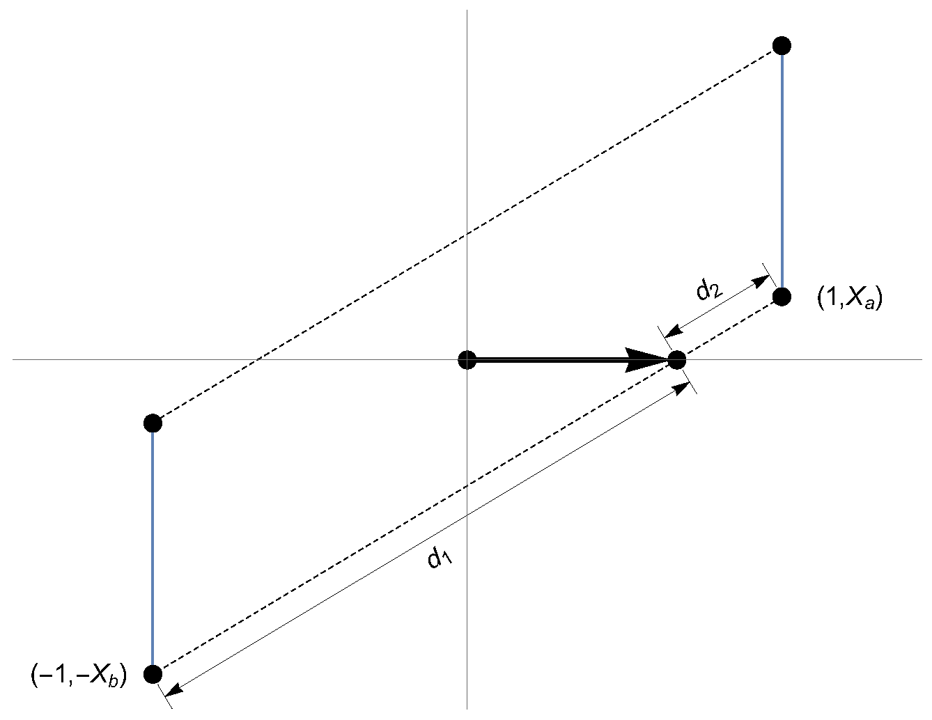
Elfving’s method is a well-known geometric procedure to obtain c-optimal designs [27]. While the method is particularly useful for two-dimensional models, its complexity increases in higher dimensions. López-Fidalgo and Rodríguez-Díaz [28] proposed a computational procedure for finding c-optimal designs that does not require the graphical construction of Elfving’s approach.

1.1.3. Filling Designs

Another commonly used approach is to use designs that cover the design space with a specific, pre-fixed, number of points, including both ends of the interval, and assign equal weights to all the support points. This type of design is denominated (space) filling designs or sequence designs. There are several ways in which the interval can be divided. Let $\mathcal{X}=\left[a,b\right]$ be the design interval, which has length $l=b-a$, and suppose n points are wanted. The simplest form is to divide the interval into equal parts, where the distance between every pair of consecutive design points is $d=l/(n-1)$. These are known as uniform designs. Another kind of filling designs is parabolic designs, which offer the possibility to concentrate samples near a particular point of the interval. To compute a parabolic design, first, the interval $[-1,1]$ is divided by n equally spaced points, which are projected into a parabola of curvature k and then projected back, giving points $(v,q)$. The values of k and q regulate the dispersion of the points, while v ($-1\le v\le 1$) controls where the concentrations of points occurs (−1: near a, 0: center of the interval, 1: near b). Then, the support points are calculated as $a+\frac{P_i-P_1}{P_n-P_1}l$, with $P_i=\left(p_{i}q\right)/(q-k{p}_i^2)$ and $p_i=2(i-1)/(n-1)-1-v$. More details on the calculations of filling designs can be found in [29] and their application in [30].

2. Accelerated Failure Time Models

AFT models can be mathematically expressed making use of the survival function,

$$S(t\mid \mathbf{x},\mathit{\theta })=S_u(t·AF(\mathbf{x},\mathit{\theta })),$$

(4)

where the survival function under conditions $\mathbf{x}$ is represented by S and $S_u$ is the baseline survival function under usual conditions. The acceleration factor is $AF(x,\mathit{\theta })$, which speeds up the effect of the survival time and depends on parameters $\mathit{\theta }$. Let $T_x$ represent the survival time subject to conditions x and $T_u$ in usual conditions. Loosely speaking, the time-to-failure under conditions x is equal to the time-to-failure in usual conditions divided by the acceleration factor, precisely $T_x=T_u/AF(x,\mathit{\theta })$. Both T and $T_u$ follow the same distribution. Then:

$$\mathbb{P}(T_x\le t)=\mathbb{P}(T_u\le t·AF(\mathbf{x},\mathit{\theta }))),$$

(5)

that is, when $AF(\mathbf{x},\mathit{\theta })\ge 1$, then, $T_x<T_u$.

Taking logarithms:

$$\begin{array}{ccc}\hfill \mathbb{P}(T_x\le t)& =& P(log\left(T_x\right)\le log\left(t\right)),\hfill \\ & =& \mathbb{P}(T_u\le t·AF(\mathbf{x},\mathit{\theta })))\hfill \\ & =& \mathbb{P}(log\left(T_u\right)\le log\left(t\right)+log\left(AF(\mathbf{x},\mathit{\theta })\right))\hfill \\ & =& \mathbb{P}\left(\frac{log\left(T_u\right)-\mu }{\sigma }\le \frac{log\left(t\right)-\mu +log\left(AF\right(\mathbf{x},\mathit{\theta }\left)\right)}{\sigma }\right)\hfill \\ & =& \mathbb{P}(ϵ\le \frac{log\left(t\right)-\mu +log\left(AF\right(\mathbf{x},\mathit{\theta }\left)\right)}{\sigma })\hfill \\ & =& \mathbb{P}(\mu -log(AF(\mathbf{x},\mathit{\theta }))+\sigma ϵ\le log(t\left)\right),\hfill \end{array}$$

with $\mu =\mathbb{E}\left[log\left(T_u\right)\right]$ and ${\sigma }^2=\mathrm{Var}\left[log\left(T_u\right)\right]$. The expression $ϵ=\frac{log\left(T_u\right)-\mu }{\sigma }$ represents a random variable with a particular distribution and mean zero:

$$\begin{array}{ccc}\hfill S(t\mid \mathbf{x},\mathit{\theta })& =& S_{ϵ}\left(\left.\frac{log\left(t\right)-\mu +log\left(AF\right(\mathbf{x},\mathit{\theta }\left)\right)}{\sigma }\right|\mathbf{x},\mathit{\theta }\right),\hfill \end{array}$$

(6)

$$\begin{array}{ccc}\hfill f(t\mid \mathbf{x},\mathit{\theta })& =& \frac{1}{\sigma t}{f}_{ϵ}\left(\left.\frac{log\left(t\right)-\mu +log\left(AF\right(\mathbf{x},\mathit{\theta }\left)\right)}{\sigma }\right|\mathbf{x},\mathit{\theta }\right).\hfill \end{array}$$

(7)

For each distribution of $ϵ$, there is a corresponding distribution for T, and vice versa.

The log-linear form of the model is:

$$log\left(T_x\right)=\mu -log\left(AF(x,\mathit{\theta })\right)+\sigma ϵ.$$

(8)

This form is implemented in most software packages.

In the following sections, two types of acceleration factors related to chemical degradation of products are considered. The rate of the chemical reaction that produces the degradation increases with temperature, thus decreasing the survival time of the product/component (for example, the plastic cover of wires in an electric device). The popular Arrhenius and Eyring equations relating the reaction rate with temperature are described and studied in order to obtain the corresponding acceleration factors.

2.1. Arrhenius Relationship

Introduced by Arrhenius [31] in his studies of the dissociation of electrolytes, it is broadly used to measure how the rate of a chemical reaction is affected by changes in temperature. The rate of a process in terms of the temperature, $\mathsf{temp}$, can be written:

$$R_{Ar}\left(\mathsf{temp}\right)={\gamma }_{0}exp\left[-\mathrm{11,605}{E}_a/\mathsf{temp}\right],$$

(9)

where the parameters are independent of temperature. The frequency factor ${\gamma }_0$ is a constant, and $E_a$ is the activation energy that represents the energy that a molecule must achieve in order to take part in the chemical reaction. This activation energy is a characteristic of the product or material, and it is measured in electron-volts. The information on $E_a$ is generally available from previous experience, physical/chemical knowledge, handbooks, etc. For many consumer electronics products, $E_a$ is roughly within some typical ranges.

Let ${\mathsf{temp}}_u$ be the usual temperature of use of the material or product (in Kelvin degrees) and $\mathsf{temp}$ the experimental temperature; the Arrhenius acceleration factor is:

$$A{F}_{Ar}({\mathsf{temp}}_u,\mathsf{temp},E_a)=\frac{R_{Ar}\left(\mathsf{temp}\right)}{R_{Ar}\left({\mathsf{temp}}_u\right)}=exp\left[\mathrm{11,605}{E}_a\left(\frac{1}{{\mathsf{temp}}_u}-\frac{1}{\mathsf{temp}}\right)\right].$$

(10)

In this case, the rate, $R_{Ar}$, is inversely proportional to the expected failure time (as the velocity of the reaction increases, so does the degradation of the product, and thus, the expected failure time shortens). Therefore, $A{F}_{Ar}=\frac{\mathbb{E}\left[T_u\right]}{\mathbb{E}\left[T_x\right]}\equiv \frac{R_{Ar}\left(\mathsf{temp}\right)}{R_{Ar}\left({\mathsf{temp}}_u\right)}$.

The Arrhenius relationship does not apply to all temperature acceleration problems, but is widely and satisfactorily used in many applications [2].

2.2. Eyring Relationship

The Arrhenius model requires that the rate of a reaction increases monotonically with temperature. Eyring and Lin [32] gave a physical theory that describes the effect that temperature has on a reaction rate, based on the Arrhenius relationship, which was discovered through empirical observation. Written in terms of a reaction rate, the Eyring relationship is:

$$R_{Ey}\left(\mathsf{temp}\right)={\mathsf{temp}}^m{R}_{Ar}\left(\mathsf{temp}\right),$$

(11)

The Eyring acceleration factor is:

$$A{F}_{Ey}({\mathsf{temp}}_u,\mathsf{temp},E_a)=\frac{R_{Ey}\left(\mathsf{temp}\right)}{R_{Ey}\left({\mathsf{temp}}_u\right)}={\left(\frac{\mathsf{temp}}{{\mathsf{temp}}_u}\right)}^{m}A{F}_{Ar}({\mathsf{temp}}_u,\mathsf{temp},E_a).$$

(12)

The value of m usually ranges between zero and one. It is important to be aware that the estimate of $E_a$ depends strongly on the assumed value of m when the data are limited [2], and only with great amounts of data can the effects of $E_a$ and m be split. The Eyring relationship leads to better low-stress extrapolations when m can be determined accurately on the basis of physical considerations.

3. Optimal Design Calculation for AFT Models with Type I Censoring and Known Variance

As mentioned in Section 2, for each distribution of $ϵ$, there is a corresponding distribution for T. In this paper, $ϵ$ is assumed to follow a standard normal distribution, and thus, the variable time-to-failure T follows a log-normal distribution.

Products that do not fail during the period of study are said to have a censored observation. A type I censoring situation occurs when the failure of a product is not observed, but it is known that this event takes place later than a given point in time. The end of the study at time d is the only censoring considered, marked by the indicator variable $\delta \equiv 1_{\{T<d\}}$ ($\delta =1$ if $T<d$ and $\delta =0$ if $T>d$).

3.1. Arrhenius Acceleration Factor

Substituting the Arrhenius relationship (10) in the log-linear form of the model (8):

$$\begin{array}{ccc}\hfill log\left(T_x\right)& =& \mu -log\left(AF\right(x,\mathit{\theta }\left)\right)+\sigma ϵ\hfill \\ & =& \mu -\mathrm{11,605}{E}_a\left(1/{\mathsf{temp}}_u-1/\mathsf{temp}\right)+\sigma ϵ\hfill \\ & =& \mu +\theta x+\sigma ϵ,\hfill \end{array}$$

where:

$$\begin{array}{ccc}\hfill x& =& \left(\frac{1}{{\mathsf{temp}}_u}-\frac{1}{\mathsf{temp}}\right),\hfill \end{array}$$

(13)

$$\begin{array}{ccc}\hfill \theta & =& -\mathrm{11,605}{E}_a.\hfill \end{array}$$

(14)

Note that $\theta$ is a negative number and x is a real number with a modulus that increases as the distance between temp and temp${}_u$ increases. With this notation, the acceleration factor can be expressed as $A{F}_{Ar}\left(x\right)=e^{-\theta x}$. Then, the log-likelihood function for just one observation value is:

$$\begin{array}{ccc}\hfill LL(\mu ,\theta ;t,x)& =& \delta log\left(f\right(t\mid x,\theta \left)\right)+(1-\delta )log\left(S\right(d\mid x,\theta \left)\right)\hfill \\ & =& -\delta log\left(\sigma t\right)+\delta log\left(f_{ϵ}\left(z_t\right)\right)+(1-\delta )log\left(S_{ϵ}\left(z_d\right)\right),\hfill \end{array}$$

(15)

where:

$$z_t={\displaystyle \frac{log\left(t\right)-\mu -\theta x}{\sigma }},$$

(16)

and $S_{ϵ}$ and $f_{ϵ}$ are the survival function and probability density function of $ϵ$, respectively:

$$\begin{array}{ccc}\hfill S(t\mid x,\theta )& =& S_{ϵ}\left(z_t\right);\hfill \\ \hfill f(t\mid x,\theta )& =& \frac{1}{\sigma t}{f}_{ϵ}\left(z_t\right).\hfill \end{array}$$

Following the results presented by Rivas-López et al. [33] and assuming known variance, the FIM for one particular observation is:

$$I(\mu ,\theta ;x)=\left(\begin{array}{cc}A\left(x\right)& xA\left(x\right)\\ xA\left(x\right)& x^{2}A\left(x\right)\end{array}\right),$$

(17)

where:

$$A\left(x\right)=\frac{1}{{\sigma }^2}\left[{\displaystyle \frac{f_{ϵ}{\left(z_d\right)}^2}{S_{ϵ}\left(z_d\right)}}+{\int }_{-\infty }^{z_d}{\displaystyle \frac{f_{ϵ}^{\prime }{\left(z\right)}^2}{f_{ϵ}\left(z\right)}}dz\right].$$

(18)

Let $\varphi$ and $\mathsf{\Phi }$ represent the probability density function of the standard normal distribution and the cumulative distribution function, respectively. In this case, ${\varphi }^{\prime }\left(z\right)=-z\varphi \left(z\right)$, and the integration gives $A\left(x\right)$ proportional to:

$$\varphi \left(z_d\right)\left[{\displaystyle \frac{\varphi \left(z_d\right)}{1-\mathsf{\Phi }\left(z_d\right)}}-z_d\right]+\mathsf{\Phi }\left(z_d\right).$$

(19)

Letting:

$$y\equiv z_d={\displaystyle \frac{log\left(d\right)-\mu -\theta x}{\sigma }},$$

(20)

then the designs that would result for this information matrix are equivalent to those calculated for the linear model with regressors:

$$\sqrt{\varphi \left(y\right)\left[{\displaystyle \frac{\varphi \left(y\right)}{1-\mathsf{\Phi }\left(y\right)}}-y\right]+\mathsf{\Phi }\left(y\right)}\left(\begin{array}{c}1\\ y\end{array}\right).$$

(21)

Therefore, for a two-point D-design $\xi$ with equal weights, the FIM is:

$$\begin{array}{ccc}\hfill M(\mu ,\theta ,\xi )& =& \sum _{i=1}^2\frac{1}{2}A\left(y_i\right)\left(\begin{array}{cc}1& y_i\\ y_i& y_i^2\end{array}\right)\hfill \\ & =& \frac{1}{2}\left(\begin{array}{cc}A\left(y_1\right)+A\left(y_2\right)& y_{1}A\left(y_1\right)+y_{2}A\left(y_2\right)\\ y_{1}A\left(y_1\right)+y_{2}A\left(y_2\right)& y_1^{2}A\left(y_1\right)+y_2^{2}A\left(y_2\right)\end{array}\right).\hfill \end{array}$$

(22)

To obtain the D-optimal design, one must maximize the determinant of the FIM:

$$detM(\mu ,\theta ,\xi )\approx A\left(y_1\right)A\left(y_2\right){(y_1-y_2)}^2.$$

(23)

Note that if $\mathsf{temp}>{\mathsf{temp}}_u$, then $x\in \left[x_a,x_b\right]$ with $x_i=\left(1/{\mathsf{temp}}_u-1/{\mathsf{temp}}_i\right)$, and hence, taking into account that $\theta <0$, $y\in \left[y_a,y_b\right]$, with $y_i=\frac{log\left(d\right)-\mu -\theta x_i}{\sigma }$ (if $\mathsf{temp}<{\mathsf{temp}}_u$, then $y\in \left[y_b,y_a\right]$). Figure 1 shows that the determinant has a valley shape and will therefore be maximized at the extremes of the interval.

Figure 1. Shape of the determinant of the FIM for a two-point equally weighted design. On the left, contour lines mark the unit-by-unit increments in the determinant. On the right, an angle of the 3D perspective is shown.

3.2. Eyring Acceleration Factor

As above, let:

$$\begin{array}{ccc}\hfill x& =& \left(\frac{1}{{\mathsf{temp}}_u}-\frac{1}{\mathsf{temp}}\right),\hfill \\ \hfill \theta & =& -\mathrm{11,605}{E}_a.\hfill \end{array}$$

The Eyring acceleration factor can be written as:

$$\begin{array}{ccc}\hfill A{F}_{Ey}({\mathsf{temp}}_u,\mathsf{temp},E_a)& =& {(1-{\mathsf{temp}}_{u}x)}^{-m}A{F}_{Ar}({\mathsf{temp}}_u,\mathsf{temp},E_a)\hfill \\ & =& {(1-{\mathsf{temp}}_{u}x)}^{-m}exp(-\theta x).\hfill \end{array}$$

(24)

The log-linear form of Model (8) is now:

$$\begin{array}{ccc}\hfill log\left(T_x\right)& =& \mu -log\left(AF\right(x,\theta \left)\right)+\sigma ϵ\hfill \\ & =& \mu +\theta x+mlog(1-{\mathsf{temp}}_{u}x)+\sigma ϵ,\hfill \end{array}$$

Letting:

$$y\equiv z_d={\displaystyle \frac{log\left(d\right)-\mu -\theta x-mlog(1-{\mathsf{temp}}_{u}x)}{\sigma }},$$

(25)

in (18) and assuming that m is known, the FIM has the expression (22). Applications in the literature have typically used $m=0$, which reduces the relationship to the Arrhenius acceleration factor, $m=0.5$ [34] and $m=1$ [23]. For these values (in fact, for any $m>0$), the expression $-mlog(1-{\mathsf{temp}}_{u}x)$ increases with x and thus with temp (provided that temp > temp${}_u$).

3.3. D-Optimal Design for AFT Models

From (13), x increases as $\mathsf{temp}$ increases, and since $\theta <0$, there is the same relationship between y and x. Thus, when the optimal design takes the two extreme values of the design interval for y, it would take as well the extreme values of the design interval for $\mathsf{temp}$ for the Arrhenius model. Furthermore, the additional expression that appears in (25) for the Eyring model does not change the pattern, and therefore, regardless of the Acceleration Factor chosen, the D-optimal design will be:

$${\xi }_{AFT}^{*}=\left\{\begin{array}{cc}{\mathsf{temp}}_a& {\mathsf{temp}}_b\\ 1/2& 1/2\end{array}\right\},$$

(26)

4. New Compromise Design Plan

As mentioned in the Introduction, two-level optimal designs are not very useful in practice. Nelson and Hahn [35,36] used Monte Carlo simulations to conclude that test plans with at least three levels and the majority of samples taken at the lowest level are more robust than the optimal two-level plans. Later on, Nelson and Kielpinski [21] suggested the use of compromise plans where the extra stress levels and their allocation are selected by the practitioner. Meeker [15] showed that the three equally spaced levels’ plans (with equal allocations) and the optimal plans are less robust than the compromise plans. Later on, Meeker and Hahn [24] proposed a compromise plan with three equally spaced levels and weights $\left\{4/7,2/7,1/7\right\}$ at the lowest, middle, and highest stress levels, respectively. There have not been many changes since Meeker’s optimal compromise plan, which is widely used in engineering and used as a reference for most of the subsequent plans proposed [18].

The proposed compromised design plan presented below builds on the idea of taking advantage of the known optimal designs for the Arrhenius and Eyring equations [37,38]. These designs are (in most cases) supported at two points as well: the upper extreme and one within the design interval. These optimal designs produce the best estimate for the activation energy (the $\theta$ parameter). Moreover, the c-optimal design for the parameter $\mu$ can be calculated in order to produce the best estimate of $\mu$. A mixture of the D-optimal design for the AFT model and these two designs optimizing each parameter respectively was proposed, based on the three-point compromise plan. Rather than the third point of the design being just the middle point, this can be taken from the designs corresponding to the acceleration factor equation. Moreover, the weights can be allocated depending on the most interesting parameter from the point of view of the practitioner.

4.1. D-Optimal Design for the Arrhenius Equation

For the Arrhenius Equation (9), the D-optimal design is equally supported at two points in the design interval. If $\mathsf{temp}=\left[{\mathsf{temp}}_a,{\mathsf{temp}}_b\right]$ and ${\displaystyle \frac{{\mathsf{temp}}_a·{\mathsf{temp}}_b}{{\mathsf{temp}}_b-{\mathsf{temp}}_a}}<$ 11,605$E_a$, then:

$$t_{Ar}={\displaystyle \frac{\mathrm{11,605}{E}_a{\mathsf{temp}}_b}{\mathrm{11,605}{E}_a+{\mathsf{temp}}_b}},$$

(27)

otherwise, $t_{Ar}={\mathsf{temp}}_a$. Then:

$${\xi }_{Ar}^{*}=\left\{\begin{array}{cc}{t}_{Ar}& {\mathsf{temp}}_b\\ 1/2& 1/2\end{array}\right\}.$$

(28)

Details of the calculations can be found in Rodríguez-Aragón and López-Fidalgo [37].

4.2. D-Optimal Design for the Eyring Equation

In the case of the Eyring Equation (11), the D-optimal design is also supported at two points. Now, if $\mathsf{temp}=\left[{\mathsf{temp}}_a,{\mathsf{temp}}_b\right]$ and ${\displaystyle \frac{{\mathsf{temp}}_a·{\mathsf{temp}}_b}{{\mathsf{temp}}_b-{\mathsf{temp}}_a}}-m{\mathsf{temp}}_a<$ 11,605$E_a$, then:

$$t_{Ey}={\displaystyle \frac{2·\mathrm{11,605}{E}_a{\mathsf{temp}}_b}{\alpha +\sqrt{{\alpha }^2+4·\mathrm{11,605}{E}_a·m{\mathsf{temp}}_b}}},$$

(29)

with $\alpha =$11,605$E_a+{\mathsf{temp}}_b(1-m)$. Otherwise, $t_{Ey}={\mathsf{temp}}_a$. Then:

$${\xi }_{Ey}^{*}=\left\{\begin{array}{cc}{t}_{Ey}& {\mathsf{temp}}_b\\ 1/2& 1/2\end{array}\right\}.$$

(30)

Details of the calculations can be found in Rodríguez-Díaz and Santos-Martín [38].

4.3. c-Optimal Design for the Parameter $\mu$

The c-optimal design for the parameter $\mu$ in the AFT model is:

$${\xi }_{c1}^{*}=\left\{\begin{array}{cc}{\mathsf{temp}}_a& {\mathsf{temp}}_b\\ x_b/(x_a+x_b)& x_a/(x_a+x_b)\end{array}\right\}.$$

(31)

Details of the computation can be found in Appendix A. As $x_a$ tends to zero (${\mathsf{temp}}_a$ tends to the normal use temperature), the first weight approaches one, and as the usual situation is having the extreme of the design interval close to ${\mathsf{temp}}_u$, the c1-optimal design can be approximated to the one-point design:

$${\xi }_{\mu }^{*}=\left\{\begin{array}{c}{\mathsf{temp}}_a\\ 1\end{array}\right\}.$$

(32)

4.4. A New Mixture of Designs

In this paper, a combination of the three previous designs was proposed: let $\gamma$ represent the weight, which was assigned to the ${\xi }_{AFT}^{*}$ design (26), and $\lambda$ to the c1-optimal design, then a mixture of the designs could be:

$$\gamma {\xi }_{AFT}^{*}+(1-\gamma -\lambda ){\xi }_{AF}^{*}+\lambda {\xi }_{\mu }^{*},$$

(33)

where ${\xi }_{AF}^{*}$ represents the design for the Acceleration Factor, ${\xi }_{Ar}^{*}$ or ${\xi }_{Ey}^{*}$, depending on the relationship chosen. The resulting mixture of the three designs is:

$${\xi }_3=\left\{\begin{array}{ccc}{\mathsf{temp}}_a& t_{AF}& {\mathsf{temp}}_b\\ \frac{\gamma +2\lambda }{2}& \frac{1-\gamma -\lambda }{2}& \frac{1-\lambda }{2}\end{array}\right\},$$

(34)

with $t_{AF}$ corresponding to the appropriate point: $t_{Ar}$ or $t_{Ey}$.

It could also be considered to use only the two optimal designs for the acceleration factor and $\mu$:

$$(1-\lambda ){\xi }_{AF}^{*}+\lambda {\xi }_{\mu }^{*},$$

(35)

and so, the resulting mixture of these two designs is:

$${\xi }_2=\left\{\begin{array}{ccc}{\mathsf{temp}}_a& t_{AF}& {\mathsf{temp}}_b\\ \lambda & \frac{1-\lambda }{2}& \frac{1-\lambda }{2}\end{array}\right\},$$

(36)

5. Numerical Example

Liu and Tang [39] proposed a Bayesian inference method to estimate the model parameters of a Device A being tested by accelerating its failure time by high temperatures. The data were presented in Hooper and Amster [40] and also available in Meeker and Escobar [20]. In their scheme, the testing units, which had a normal temperature of 283 K, were tested at three accelerated temperatures: 313 K, 333 K, and 353 K, and the number of failures within a censoring time of 5000 h was observed. They also assumed $\sigma$ to be known and fixed it at $0.7$, its maximum likelihood estimate. Their estimates of $\mu$ for each of the used temperatures were, respectively, 7.48, 8.81, and 10.13. In this case, the engineering knowledge suggested $E_a\in \left[0.5,0.8\right]$. In their design, they allocated $75\%$ of the units to the lowest temperature, $15\%$ to the second, and the final $10\%$ to the highest temperature.

To calculate the designs proposed in Section 3 and Section 4, let:

• usual temperature of use ${\mathsf{temp}}_u=283\mathrm{K}$,
• design interval $\mathsf{temp}\in \left[313\mathrm{K},353\mathrm{K}\right]$,
• censoring time, $d=5000\mathrm{h}$,
• $\mu =\mathrm{E}\left[log\left(T_u\right)\right]=8.81$ (mean of the three estimates in Liu and Tang [39]),
• $\sigma =\mathrm{Var}\left[log\left(T_u\right)\right]=0.7$,
• energy of activation $E_a=0.65$.

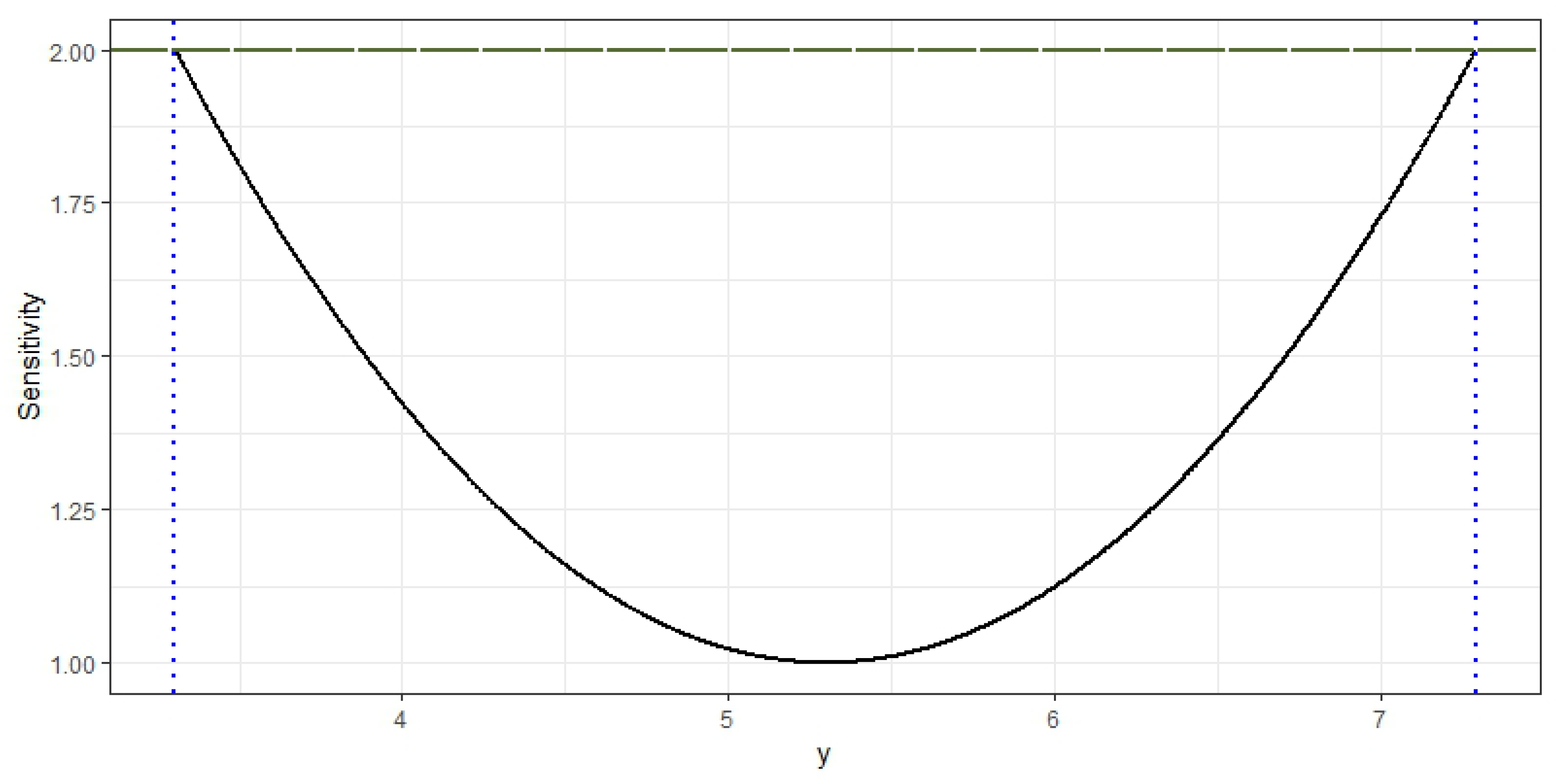
The D-optimal design for the AFT model is the equally weighted design supported at both extremes of the interval. The sensitivity Function (2), shown in Figure 2, remains smaller than two (the number of parameters) in the whole design space, and so, the obtained design is indeed D-optimal. Furthermore, the maxima are reached at the support points (i.e., the extremes of the interval). The three optimal designs are shown in Table 1.

Figure 2. Sensitivity function for the D-optimal design for the AFT model, over the y interval. Maxima, located at the support points (the extremes), are marked by dotted lines.

Table 1. D-optimal designs for the AFT model and the Arrhenius and Eyring ($m=0.5$) equations and c-optimal design for the parameter $\mu$ in the AFT model.

AFT Model	Acceleration Factor	Parameter $\mathit{\mu }$
${\xi }_{AFT}^{*}=\left\{\begin{array}{cc}313& 353\\ 1/2& 1/2\end{array}\right\}$	${\xi }_{Ar}^{*}=\left\{\begin{array}{cc}337.2192& 353\\ 1/2& 1/2\end{array}\right\}$	${\xi }_{\mu }^{*}=\left\{\begin{array}{c}313\\ 1\end{array}\right\}$
	${\xi }_{Ey}^{*}=\left\{\begin{array}{cc}337.5495& 353\\ 1/2& 1/2\end{array}\right\}$

For values of m between zero and one, $t_{Ey}$ varies from $337.2192$ (m = 0, equivalent to the Arrhenius equation) to $337.8667$, so the points move slowly towards higher values. However, due to the closeness to the Arrhenius equation, we shall focus from now on on the designs using $t_{Ar}=337.2192$.

Mixtures of the three designs, calculated using (34), were studied for different values of $\gamma$ and $\lambda$. Table 2 shows the weights of the support points ${\xi }_3=\left\{313337.2192353\right\}$ for different combinations of the designs with the determinants of the FIM shown in parentheses.

Table 2. Weights for the mixture design ${\xi }_3$ for different values of $\gamma$ and $\lambda$ and their corresponding determinant of the FIM (in parentheses).

	$\mathit{\lambda }$	0.1	0.3	0.5	0.7
$\mathit{\gamma }$
0.2		$\left\{0.20.350.45\right\}$	$\left\{0.40.250.35\right\}$	$\left\{0.60.150.25\right\}$	$\left\{0.80.050.15\right\}$
		$\left(2.12\right)$	$\left(2.92\right)$	$\left(2.91\right)$	$\left(2.09\right)$
0.4		$\left\{0.30.250.45\right\}$	$\left\{0.50.150.35\right\}$	$\left\{0.70.050.25\right\}$
		$\left(2.74\right)$	$\left(3.23\right)$	$\left(2.90\right)$
0.6		$\left\{0.40.150.45\right\}$	$\left\{0.60.050.35\right\}$
		$\left(3.24\right)$	$\left(3.42\right)$
0.8		$\left\{0.50.050.45\right\}$
		$\left(3.62\right)$

In Liu and Tang [39], most of the observations were taken near the lower extreme of the interval, i.e., the temperature closer to the usual. Their three-point design had three equally spaced points, at temperatures 313 K, 333 K, and 353 K, with weights $75\%$, $15\%$, and $10\%$, which follows a similar idea as the “4:2:1 plan”.

It can be noted that the designs in Table 3 have smaller values for the determinant of the FIM matrix (shown in brackets), which implies they are less efficient designs, according to the D-optimal criterion. In fact, taking, for example, $\gamma =0.6$ and $\lambda =0.3$, their D-efficiency (3) with respect to the mixture design, ${\xi }_3$, is $69.99\%$ for Liu and Tang’s design and $78\%$ for the 4:2:1 design.

Table 3. Three-point designs with weights concentrated at the lower end and their corresponding determinant of the FIM (in parentheses).

Liu and Tang Design	4:2:1 Plan Design
$\xi =\left\{\begin{array}{ccc}313& 333& 353\\ 0.75& 0.15& 0.10\end{array}\right\}$	$\xi =\left\{\begin{array}{ccc}313& 333& 353\\ 4/7& 2/7& 1/7\end{array}\right\}$
$\left(1.67\right)$	$\left(2.08\right)$

Table 4 shows some filling designs for the AFT model. A parabolic design that concentrates points at the beginning of the interval was considered, to account for the concentration of points at lower temperatures. It can be seen that adding an extra support point ($n=4$) did not improve the design (in terms of D-optimality), but these filling designs are actually more efficient than the ones shown in Table 3. The D-efficiency of Liu and Tang’s design, with respect to the three-point uniform and parabolic design presented, was $81.16\%$ and $78.56\%$, respectively. The D-efficiency of the 4:2:1 design with respect to the uniform design was $90.45\%$ and $87.55\%$ with respect to the parabolic design. Taking again $\gamma =0.6$ and $\lambda =0.3$ as an example, the D-efficiency of the three-point filling designs with respect to the mixture design, ${\xi }_3$, was $86.23\%$ for the uniform design and $89.09\%$ for the parabolic design.

Table 4. Filling designs with three and four support points and their corresponding determinant of the FIM (in parentheses).

	Uniform Designs	Parabolic Designs $\mathit{k}=\mathbf{1},\mathit{q}=\mathbf{7},\mathit{v}=-\mathbf{1}$
n = 3	$\xi =\left\{\begin{array}{ccc}313& 333& 353\\ 1/3& 1/3& 1/3\end{array}\right\}$	$\xi =\left\{\begin{array}{ccc}313& 323& 353\\ 1/3& 1/3& 1/3\end{array}\right\}$
	$\left(2.54\right)$	$\left(2.71\right)$
n = 4	$\xi =\left\{\begin{array}{cccc}313& 326.33& 339.67& 353\\ 1/4& 1/4& 1/4& 1/4\end{array}\right\}$	$\xi =\left\{\begin{array}{cccc}313& 319.10& 328.32& 353\\ 1/4& 1/4& 1/4& 1/4\end{array}\right\}$
	$\left(2.12\right)$	$\left(2.18\right)$

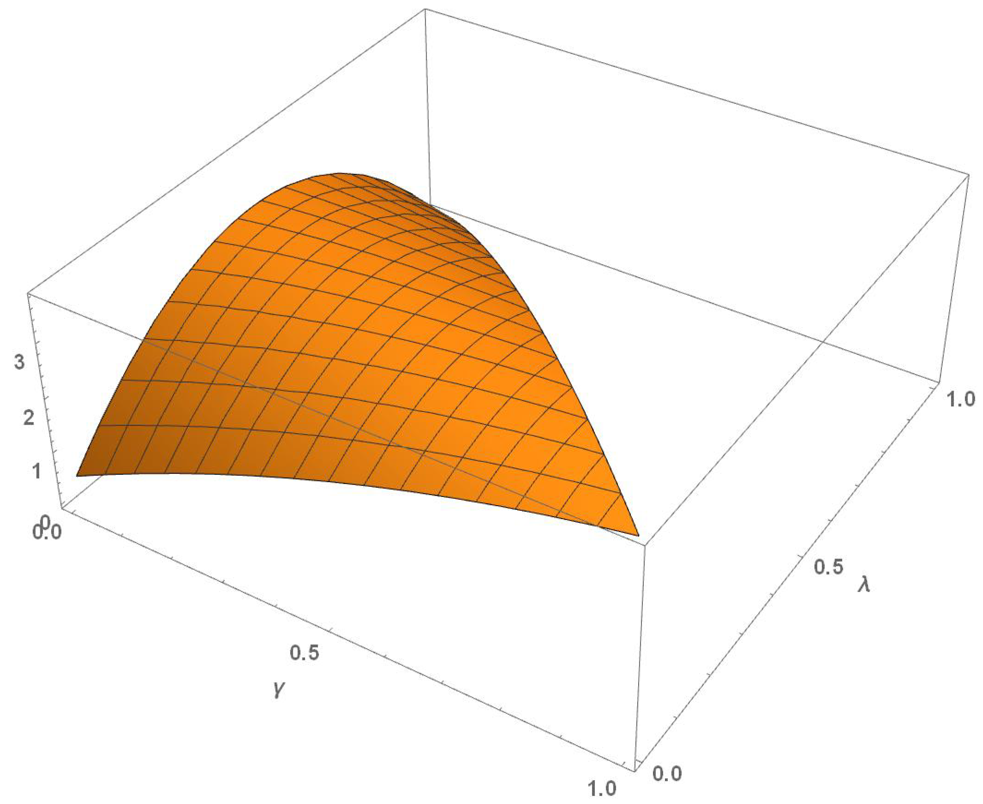
The determinant of the FIM of the mixture design ${\xi }_3$ can be expressed as a function of $\gamma$ and $\lambda$ as:

$$\mathrm{Det}\left[M({\xi }_3,\theta )\right]=-1.5285{\gamma }^2-7.8801\gamma \lambda +4.8231\gamma -10.1564{\lambda }^2+9.6462\lambda +0.5102,$$

which is shown in Figure 3.

Figure 3. Determinant of the FIM of the mixture design ${\xi }_3$ as a function of $\gamma$ and $\lambda$.

The maximum value, 3.80482, was attained for $\gamma =1$ and $\lambda =0$, that is without using ${\xi }_{\mu }^{*}$ in the mixture design. Nevertheless, the use of ${\xi }_{\mu }^{*}$ provides a way to “tune” the design according to the expertise of the practitioner when a higher weight at the lower extreme of the design interval seems convenient.

6. Discussion

AFT models were first introduced in engineering, but their use has become increasingly popular as an alternative to proportional hazard models, also in the medical field [33]. As important as it is that accelerated test programs are planned and conducted by teams with good knowledge about the material/product, the typical use conditions, and the physical/chemical/mechanical aspects of the failure models, it is also important to take into account the statistical aspects of the design and analysis of reliability experiments [2].

In this paper, the methodology to obtain optimal designs for an AFT model was presented. In particular, the details when assuming a log-normal distribution for the survival time and considering the case of known variance were shown. Optimal design uses different criteria related to the variance of the estimators to select observational points in which to obtain the best estimates of a model’s parameters. The most commonly used criterion, D-optimality, was considered. The D-optimal designs are supported at the extremes of the intervals, and although the two-point D-optimal design is better than a three-point design, a design in the boundaries of the interval may not always be useful. Moreover, these designs are not very robust [19]. For these reasons, a new approach was presented, where the D-optimal design for the AFT model can be combined with the D-optimal design that produced the best estimates for the acceleration factor chosen (Arrhenius or Eyring) and the best design for estimating the parameter $\mu$, the expected value of the survival time under usual conditions (in logarithm scale). In the proposed mixture of designs, the experimenter can decide where to put the emphasis by selecting different values of $\lambda$ and $\gamma$. The three-point mixture design proposed was studied in comparison to the design proposed by Liu and Tang [39], the “4:2:1 plan” design plan, the use of which is widely extended, and different filling designs. The design proposed had a higher D-efficiency than the others. It can be thought that having a higher number of support points along the design interval would lead to better estimations of the parameters. Nonetheless, the four-point filling designs shown had lower efficiencies than the three-point ones.

As described by Meeker and Escobar [20], accelerated tests should be designed, as much as possible, to minimize the amount of extrapolation required. This means that levels of accelerating variables that are too high may result in failure models that would never actually occur at the use levels of the accelerating models. For this reason, the approximation of the c-optimal design to the single point design at the lowest end of the design interval acts as a penalty to extreme temperature values. The mixture designs proposed in this paper seemed to be a good alternative to the compromise plans, improving them by choosing a support point in the interval that was optimal for the acceleration factor, rather than simply the middle point. Furthermore, the weights can be adjusted depending on the parameter in which the practitioner is more interested.

7. Conclusions and Future Work

This paper aimed to improve the traditionally used compromise design plans for AFT models. As previously mentioned, the two-level optimal design is not always practical, and there have not been many changes since the “4:2:1 plan”, broadly used in engineering, was introduced.

The presented mixture design proposed to select the middle point of the design to be taken from the designs corresponding to the acceleration factor equation. Furthermore, the weights can be allocated depending on the most interesting parameter from the point of view of the practitioner. It was shown that the proposed design performed better in terms of the D-efficiency. The participation of the c optimal design for the mean parameter in this mixture design is not essential, but can help the practitioner adjust the weights of the designs points from a convenient point of view.

Several extensions are being considered as future lines of research, including: sensitivity studies regarding the initial parameters; the choice of m and/or other distributions; consideration of m as an unknown parameter to be estimated (in this case, the dimensions of the information matrix would increase and, therefore, the difficulty of the computations); and similarly, considering ${\sigma }^2$ as an unknown parameter to be estimated. In the last case, the modification of the information matrix described in Pázman [41] could be used. Furthermore, it may happen that the “controlled variable” ($\mathsf{temp}$) could not be completely fixed. In this case, extensions of D-optimal designs can be used following the ideas of Pronzato [42].