Caustic Frequency in 2D Stochastic Flows Modeling Turbulence

Abstract

Stochastic flows mimicking 2D turbulence in compressible media are considered. Particles driven by such flows can collide and we study the collision (caustic) frequency. Caustics occur when the Jacobian of a flow vanishes. First, a system of nonlinear stochastic differential equations involving the Jacobian is derived and reduced to a smaller number of unknowns. Then, for special cases of the stochastic forcing, upper and lower bounds are found for the mean number of caustics as a function of Stokes number. The bounds yield an exact asymptotic for small Stokes numbers. The efficiency of the bounds is verified numerically. As auxiliary results we give rigorous proofs of the well known expressions for the caustic frequency and Lyapunov exponent in the one-dimensional model. Our findings may also be used for estimating the mean time when a 2D Riemann type partial differential equation with a stochastic forcing loses uniqueness of solutions.

1. Introduction

We address a stochastic flow [1] covered by the following Ito stochastic differential equations

$$d\mathbf{r}=\mathbf{v}dt,d\mathbf{v}=-(\mathbf{v}/\tau )dt+d\mathbf{w}(t,\mathbf{r}),$$

(1)

where phase variables $\mathbf{r}=(x,y)$ and $\mathbf{v}=(u,v)$ are interpreted as the position and velocity of fluid particles moving in a turbulent flow. Here the random forcing $\mathbf{w}(t,\mathbf{r})$ is assumed to be a Gaussian white noise in time and a statistically homogeneous random field in space, i.e.,

$$E\mathbf{w}(t_1,{\mathbf{r}}_1)\mathbf{w}{(t_2,{\mathbf{r}}_2)}^T=min(t_1,t_2)\mathbf{B}({\mathbf{r}}_1-{\mathbf{r}}_2),$$

where $\mathbf{B}\left(\mathbf{r}\right)$ is its space covariance matrix. A constant non-random parameter $\tau$ is called the Lagrangian correlation time.

In particular, the motion of a single particle in the framework (1) is covered by a Langevin equation for the velocity

$$d\mathbf{v}=-(\mathbf{v}/\tau )dt+\mathbf{B}{\left(\mathbf{0}\right)}^{1/2}d\mathbf{w}\left(t\right)$$

where $\mathbf{w}\left(t\right)$ is a standard Brownian motion in 2D, thereby the Lagrangian velocity of the particle is simply a well known (two-dimensional) Ornstein–Uhlenback process and its position is an integrated Ornstein–Uhlenback process.

In general the motion of any number n of the particles is described by a diffusion process in $R^{2n}$ for the vector of positions/velocities $({\mathbf{r}}_1,{\mathbf{v}}_1,\dots ,{\mathbf{r}}_n,{\mathbf{v}}_n)$ with a drift and diffusivity matrix expressed in terms of $\tau$ and $\mathbf{B}$ [2].

To introduce the problem we focus on, let us supply (1) with initial conditions ${\mathbf{r}|}_{t=0}{=\mathbf{a},\mathbf{v}|}_{t=0}={\mathbf{u}}_0\left(\mathbf{a}\right)$ where ${\mathbf{u}}_0\left(\mathbf{a}\right)$ is a given deterministic function (the initial Eulerian velocity field), i.e., each particle starts from a certain position with a certain velocity completely determined by its position, and introduce the Jacobian

$${\displaystyle J(t,\mathbf{a})=det\left(\frac{\partial \mathbf{r}(t,\mathbf{a})}{\partial \mathbf{a}}\right)}$$

where $\mathbf{r}(t,\mathbf{a})$ is the solution of (1) satisfying the above initial conditions or, in simple words, the position of the particle at moment t starting $(t=0)$ at position $\mathbf{a}$.

An important physical meaning of the Jacobian can be seen from the following. Let the initial position $\mathbf{a}$ be a random variable independent of the flow with probability density ${\pi }_a\left(\mathbf{x}\right)$, then for the conditional density ${\pi }_{\mathbf{r}(t,\mathbf{a})}\left(\mathbf{x}\right)$ conditioned on the flow is given by

$${\pi }_{\mathbf{r}(t,\mathbf{a})}\left(\mathbf{x}\right)={\pi }_a\left(\mathbf{x}\right)/J(t,\mathbf{x})$$

It is well known [3] that for incompressible flows $J(t,\mathbf{a})\equiv 1$, hence the density of the particles does not change at any point in the fluid. A remarkable and one of the most important feature of model (1) is that it yields a compressible flow for any value of $\tau$ and any function ${\mathbf{u}}_0\left(\mathbf{a}\right)$, e.g., [4]. Moreover, $J(t,\mathbf{a})$ may take zero values leading to an infinite density at certain points of the fluid called caustics.

Let $\nu$ be the mean frequency (intensity) of caustic occurrence and

$${\displaystyle \lambda =\underset{t\to \infty }{lim}\frac{1}{t}\underset{\left|\mathbf{a}\right|\to 0}{lim}ln\left(\frac{\left|\mathbf{r}\right(t,\mathbf{a})-\mathbf{r}(t,\mathbf{0}\left)\right|}{\left|\mathbf{a}\right|}\right)}$$

(2)

the top Lyapunov exponent (LE) for (1).

Despite numerous studies of this important quantity in physical literature (see recent comprehensive reviews in [4,5]) almost all remarkable analytical results were obtained in the one dimensional case, among them explicit expressions [6,7] should be mentioned first

$${\displaystyle \nu =\frac{1}{2{\pi }^2\sqrt{z}M{\left(z\right)}^2},\lambda =-1+\frac{M^{\prime }\left(z\right)}{2\sqrt{z}M\left(z\right)}},$$

(3)

where $z=s^{-4/3}/4$, s is Stokes number (the ratio of Lagrangian and Eulerian time scales, e.g., [2]), M is the modulus of the Airy function. Furthermore, to our best knowledge no rigorous proofs of formulas (3) were presented so far. Furthermore, worth noting expressions for $\nu$ and $\lambda$ in a quite different setup when the noise is a telegraph process rather then the Gaussian white noise [6]. Even though that results were proven rigorously it still was a one dimensional case that hard to consider as a turbulence model.

As for two dimensions, we found no analytical results whatsoever concerning with the dependence of $\nu$ on s, while some asymptotics for LE were obtained in [2,6,7]. Moreover, exact expressions for LE were derived as well in very special degenerate cases [7].

Advances in this work could be summarized as follows.

(i) Rigorous proofs of (3) were given.

(ii) In the framework of general 2D model (1) a system of stochastic differential equations was derived in four unknowns, involving the Jacobian.

(iii) The system was efficiently investigated for two cases of a special forcing in (1) yielding an exact asymptotic of $\nu \left(s\right)$ as $s\to 0$ and reasonable numerical boundaries for $\nu \left(s\right)$ in a wide range of s. That results may be used for estimating the mean time when the corresponding SPDE for the Eulerian velocity field loses its uniqueness.

(iv) In one of that cases it was found that LE has exactly same expression as given in (3).

(v) For an isotropic turbulence the system was elaborated via introducing longitudinal and normal Stokes numbers.

In physical literature the model (1) most often was used to describe so called inertial particles such as water drops in atmospheric clouds, particulate matter or living organisms in the turbulent upper layer of oceans, and many other phenomena. Undoubtedly, real turbulent flows in the ocean and atmosphere are essentially 3D phenomena. However, the introduction of three dimensional perturbations does not destroy the main features of the cascade picture according to [8], implying that 2D turbulence phenomenology establishes a realistic picture of turbulent fluid flows.

In Eulerian terms Equation (1) cover Lagrangian motion in the Eulerian velocity field $\mathbf{u}(t,\mathbf{x})$ satisfying the following equation

$${\displaystyle \frac{\partial \mathbf{u}}{\partial t}+\mathbf{u}·\nabla \mathbf{u}+\frac{1}{\tau }\mathbf{u}=\frac{\partial \mathbf{w}}{\partial t}{,\mathbf{u}|}_{t=0}={\mathbf{u}}_0\left(\mathbf{x}\right)}.$$

(4)

By the method of characteristics one can find that for some (maybe short) interval $(0,t)$ the solution of this equation exists and unique since at the initial moment $J(0,\mathbf{a})=1$. However, after some time the uniqueness is lost (the Jacobian vanishes) due to a very weak dissipation modeled by the last term on the left hand side (LHS). Thus, estimates of the mean of the first moment when $J(t,\mathbf{a})$ hits zero would provide us with an idea when (4) loses uniqueness. In terms of the non-linear wave theory, one can treat that as the first moment of wave breaking.

Worth noting that if the dissipation term is replaced by a classical friction $k\Delta \mathbf{u}$, then we arrive at the well known stochastic Burger’s equation which has a unique solution for all t thereby no caustics may occur.

Some of our results can be predicted by simply proceeding to dimensionless variables in (4). Let U and L be some typical velocity and length scales, respectively. Changing $\mathbf{u},\mathbf{w},\mathbf{x},t$ to $\mathbf{u}/U,\mathbf{w}/U,\mathbf{x}/L,t/\tau$ one gets from (4)

$$\frac{\partial \mathbf{u}}{\partial t}+s\mathbf{u}·\nabla \mathbf{u}+\mathbf{u}=\frac{\partial \mathbf{w}}{\partial t}$$

where the dimensionless parameter

$${\displaystyle s=\frac{U\tau }{L}}$$

(5)

is called Stokes number.

Thus, if $s\to 0$ then the underlying Eulerian velocity field satisfies a linear equation and hence the intensity of caustics should tend to zero. In the opposite case $s\to \infty$ the non-linear term dominates and one may expect that the number of caustics per time grows indefinitely.

The paper is organized as follows. A similar one-dimensional problem is exactly solved in Section 1. The solution is essentially used in investigating 2D phenomena. A deterministic case ($\mathbf{w}=\mathbf{0}$) is briefly discussed in Section 2. In Section 3, we derive a system of equations containing J in the general case of an arbitrary homogeneous forcing. For particular forms of the forcing rigorous estimates for the mean number of caustics $\nu \left(s\right)$ are found in Section 4. Furthermore, $\nu \left(s\right)$ is computed by solving a simple $1D$ parabolic equation. The case of an isotropic forcing (unsolved yet) is mentioned in Section 5. Conclusions are gathered in Section 6 and some details are brought to Appendix A.

2. One-Dimensional Case

A part of results from this section is well known from physical literature [4,7,9], presented sometimes in a quite vague fashion. We formulate and prove them rigorously and give more details.

Consider

$$dx=udt,du=-(u/\tau )dt+dw(t,x),x\left(0\right)=a,u\left(0\right)=u_0\left(a\right)$$

(6)

with $Ew(t,x)=0$ and

$$Ew(t_1,x_1)dw(t_2,x_2)=min(t_1,t_2))b(x_1-x_2).$$

For

$$J(t,a)=\frac{\partial x}{\partial a}$$

one can get by direct differentiation (6) in a

$$dJ=J_{1}dt,d{J}_1=-(J_1/\tau )dt+Jd\tilde{w}\left(t\right)$$

where

$$J_1(t,a)=\frac{\partial u}{\partial a},E\tilde{w}\left(t\right)=0,E\tilde{w}{\left(t\right)}^2=-b^{″}\left(0\right)t$$

Introduce the following dimensionless quantity $p=\tau J_1/J$ and apply the Ito formula to the last system. As a result we have

$${\displaystyle dp=\frac{1}{\tau }(-p-p^2)dt+\tau d\tilde{w}\left(t\right).}$$

Then we proceed to a dimensionless time $t/\tau ⟶t$ and obtain

$${\displaystyle dp=(-p-p^2)dt+s\sqrt{2}dw\left(t\right)},$$

(7)

where w is a standard Wiener process and

$$s=\sqrt{-b^{″}\left(0\right){\tau }^3/2}.$$

(8)

Worth noting that if the velocity and length scales of the flow are chosen as $U=\sqrt{b\left(0\right)\tau }$ and $L=\sqrt{-2b\left(0\right)/b^{″}\left(0\right)}$, respectively, then (8) coincides with the earlier introduced Stokes number (5).

Assume that zeros of $J\left(t\right)$ are prime that is typical for stationary processes, then they can be identified with moments of explosion of $p\left(t\right)$.

Proposition 1.

Process p is explosive(e.g., [10]), more exactly

$$\underset{t\to S-0}{lim}p\left(t\right)=-\infty ,$$

where the explosion time S is finite

$$P(S<\infty )=1$$

and its expectation can be explicitly computed

$$E\left(S\right)=2{\pi }^2\sqrt{z}M{\left(z\right)}^2,z=s^{-4/3}/4,$$

(9)

where

$$M\left(z\right)=\sqrt{Ai{\left(z\right)}^2+Bi{\left(z\right)}^2},$$

$Ai\left(z\right),Bi\left(z\right)$ are the Airy functions and $M\left(z\right)$ their modulus.

Notice that (9) implies the expression (2) for the intensity of caustics since $\nu =1/E\left(S\right)$.

Explosiveness of $p\left(t\right)$ follows from the Feller’s criteria [10].

To prove (9) we introduce $\mu \left(x\right)$ as the mean time to explosion under condition $p\left(0\right)=x$, then solve

$$L\mu \left(x\right)=-1,\mu (-\infty )=0,$$

where

$$L=(-x-x^2)\frac{\partial }{\partial x}+s^2\frac{{\partial }^2}{\partial x^2}$$

is the generator of (7).

Then we set

$$E\left(S\right)=\mu (\infty ).$$

and arrive at (9). Details of computations are the same as in [11].

For the purpose of studying $2D$ models the knowledge of the mean explosion time is not enough. Introduce

$$\overline{F}\left(t\right)=P(S>t)$$

and let $u(t,x)$ be the same probability under condition $p\left(0\right)=x$, then

$$\overline{F}\left(t\right)=u(t,\infty ).$$

In [12], it was shown that $u(t,x)$ satisfies the initial value problem

$${\displaystyle \frac{\partial u(t,x)}{\partial t}=L_{x}u(t,x),u(0,x)=1}.$$

(10)

To ensure uniqueness of solution of (10) we add the natural boundary conditions assuming that the limit $u(t,\infty )$ exists similarly to $m(\infty )$.

$$u(t,-\infty )=0,u_x(t,\infty )=0.$$

A simplest Euler scheme was used for solving (10) numerically. Some details and validation of the choice of the scheme parameters are given in Appendix A. Notice that our goal is not to evaluate and minimize the error of the numerical computations, but rather to illustrate that (10) can be solved quite accurately and efficiently with very simple tools.

Graphs of $\overline{F}\left(t\right)$ for a few values of s are shown in Figure 1

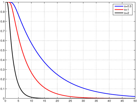
Figure 1. $P(S>t)$ versus t for $s=0.5,1,2$.

To proceed to investigating LE we notice that after explosion process $p\left(t\right)$ can be continued by starting over, i.e., by solving same Equation (7) with the initial condition

$$\underset{t\to S+0}{lim}p\left(t\right)=\infty .$$

The positive sign follows from relation $J_1=dJ/dt$ and the fact that zeros of $J\left(t\right)$ are prime. Thus, $p\left(t\right)$ takes different signs on different sides of a zero of $J\left(t\right)$.

LE for flow (7) is expressible in terms of the ergodic mean of p

$${\displaystyle \lambda =\overline{p}/\tau ,\overline{p}=\underset{t\to \infty }{lim}\frac{1}{t}{\int }_0^{t}p\left(s\right)ds}$$

as follows from (2) and definition of $p\left(t\right)$, see [2] for details. It also can be exactly found

Proposition 2.

The ergodic mean of p is given by

$$\overline{p}=-1+\frac{M^{\prime }\left(z\right)}{2\sqrt{z}M\left(z\right)}$$

(11)

The statement is proven in Appendix A and here we just make some comments. Notice that the density of the stationary distribution $\pi \left(p\right)$ of $p\left(t\right)$ does exist and is given by

$$\pi \left(p\right)=C{e}^{-p^2/2s^2-p^3/3s^2}{\int }_{-\infty }^p{e}^{y^2/2s^2+y^3/3s^2}dy$$

(12)

where C is a normalized constant.

One can find the following asymptotic

$$\pi \left(p\right)\sim {\left|p\right|}^{-2},p\to \infty .$$

Thus, the integral for the invariant mean

$$Ep={\int }_{-\infty }^{\infty }p\pi \left(p\right)dp$$

is formally divergent, however if the integral is meant as a Cauchy principal value then it coincides with the RHS of (11).

3. Deterministic 2D Case

In this section, we plug in (1) $\mathbf{w}=0$. The resulting linear equations are easy to solve and get the following expression for the Jacobian

$$J\left(t\right)=P{s}^2{\left(1-e^{-t}\right)}^2+Qs\left(1-e^{-t}\right)+1$$

in dimensionless form with Stokes number s defined in (5), where

$${\displaystyle P=\frac{\partial (u_0,v_0)}{\partial (a,b)},Q=\frac{\partial u_0}{\partial a}+\frac{\partial v_0}{\partial b}}$$

and $(a,b)$, ($u_0,v_0)$ are the initial position and velocity, respectively, related by $u_0=u_0(a,b),v_0=v_0(a,b)$.

Let

$$G=\left\{(P,Q)\right|Q^2>4P\}\bigcap \left\{(P,Q)\right|P<0\mathrm{or}\mathrm{Q}<0\}$$

and S be the first time when $J\left(S\right)=0$. Easy to find that

$${\displaystyle S=\left\{\begin{array}{cc}{\displaystyle -ln\left(1-\frac{s_0}{s}\right)}\hfill & \mathrm{if}(P,Q)\in G\mathrm{and}s>s_0\hfill \\ \\ \infty \hfill & \mathrm{otherwise}\hfill \end{array}\right.}$$

where

$${\displaystyle s_0=\frac{-Q-\sqrt{Q^2-4P}}{2P}}$$

In particular if $Q=0$ and $P<0$ do not depend on $(a,b)$ at all, then $G={\mathbb{R}}^2$ and S, defined for all $s>0$, does not depend on the initial point as well. Thus, the equation

$$\frac{\partial \mathbf{u}}{\partial t}+s\mathbf{u}·\nabla \mathbf{u}+\mathbf{u}=\mathbf{0},\mathbf{u}(0,\mathbf{x})={\mathbf{u}}_0\left(\mathbf{x}\right)$$

(13)

loses uniqueness exactly at moment $t=S$. If one defines $u(t,x)$ after $t>S$ as a solution of (13) with the initial condition

$$\mathbf{u}(S+0,\mathbf{x})={\mathbf{u}}_0\left(\mathbf{x}\right)$$

then $\nu =1/S$ could be interpreted as the intensity of caustics in time. In Figure 2, we show a few curves $\nu \left(s\right)$ for different $s_0$ in order to compare them visually with a stochastic case addressed in the next sections.

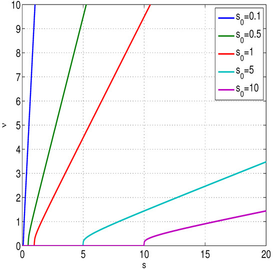
Figure 2. Dependence of the caustic rate $\nu \left(s\right)$ on Stokes number s in absence of noise.

If S depends on the initial point, then its interpretation in terms of Eulerian setup (13) is not that simple and will not be discussed here.

4. System of Equations for Jacobian in General 2D Case

Now we return to the stochastic model (1). In a few works it was pointed out that there is a closed equation for the matrix

$$\mathbf{Z}=\frac{\partial \mathbf{v}}{\partial \mathbf{a}}{\left(\frac{\partial \mathbf{r}}{\partial \mathbf{a}}\right)}^{-1}$$

Namely, e.g., [2,4]

$${\displaystyle d\mathbf{Z}=-\left(\mathbf{Z}/\tau +{\mathbf{Z}}^2\right)dt+d\left(\frac{\partial \mathbf{w}}{\partial \mathbf{a}}\right)}$$

An analysis of that equation led to some general important conclusions, but it is of little help for our purposes because in general it cannot be reduced to efficiently handled scalar equations.

Let us first rewrite (1) in the coordinate-wise form with $\mathbf{r}=(x,y),\mathbf{a}=(a,b)$

$$\begin{array}{c}du=-(u/\tau )dt+d{w}^{\left(1\right)}(t,x,y),dv=-(v/\tau )dt+d{w}^{\left(2\right)}(t,x,y),dx=udt,dy=vdt\hfill \\ \\ x\left(0\right)=a,y\left(0\right)=b,u\left(0\right)=u_0(a,b),v\left(0\right)=v_0(a,b)\hfill \end{array}$$

(14)

where

$$Ed{w}^{\left(i\right)}(t,0,0)d{w}^{\left(j\right)}(t,x,y)=b^{ij}(x,y)dt$$

and $b^{ij}$ are entries of $\mathbf{B}$. The goal is to investigate time behavior of the Jacobian

$$J\left(t\right)\equiv \frac{\partial x}{\partial a}\frac{\partial y}{\partial b}-\frac{\partial x}{\partial b}\frac{\partial y}{\partial a}$$

It is not possible to obtain a closed equation for $J\left(t\right)$, but it can be included in a system of four equation as it is shown in Appendix A. Namely, for dimensionless time $t=t/\tau$ denoted by the same letter, Jacobian can be represented as

$$J\left(t\right)=exp\left({\int }_0^t{m}_1\left(t\right)dt\right),$$

where dimensionless random function $m_1\left(t\right)$ is included into the following system

$$\begin{array}{ccc}d{m}_1\hfill & =\hfill & (-m_1+(m_4^2-m_1^2-m_2^2-m_3^2)/2)dt+sd{\eta }_1,\hfill \\ d{m}_2\hfill & =\hfill & (-m_1{m}_2-m_2)dt+sd{\eta }_2,\hfill \\ d{m}_3\hfill & =\hfill & (-m_1{m}_3-m_3)dt+sd{\eta }_3,\hfill \\ d{m}_4\hfill & =\hfill & (-m_1{m}_4-m_4)dt+sd{\eta }_4\hfill \end{array}$$

(15)

s is Stokes number defined similarly to (8) and an exact expression for it is given in Appendix A.

To define processes ${\eta }_i\left(t\right)$ we nondimensionalize $w^{\left(i\right)}\left(t\right)$ and set

$${\eta }_1=w_y^{\left(2\right)}-w_x^{\left(1\right)},{\eta }_2=w_y^{\left(2\right)}+w_x^{\left(1\right)},{\eta }_3=w_x^{\left(2\right)}-w_y^1,{\eta }_4=w_x^{\left(2\right)}+w_y^{\left(1\right)},$$

(16)

where the subs mean derivatives. Thus, $\eta$’s are dependent Wiener (non-standard) processes with a covariance matrix $Ed{\eta }^{\left(i\right)}(t,x,y)d{\eta }^{\left(j\right)}(t,x,y)={\sigma }_{\eta }^{ij}dt$ given by -4.6cm0cm

$$\left({\sigma }_{\eta }^{ij}\right)=\left(\begin{array}{cccc}-b_{xx}^{11}-b_{yy}^{22}+2b_{xy}^{12}\hfill & -b_{yy}^{22}+b_{xx}^{11}\hfill & b_{xx}^{12}+b_{yy}^{12}\hfill & b_{xx}^{12}-b_{yy}^{12}\hfill \\ -b_{yy}^{22}+b_{xx}^{11}\hfill & -b_{xx}^{11}-b_{yy}^{22}-2b_{xy}^{12}\hfill & -b_{xx}^{12}+b_{yy}^{12}\hfill & -b_{xx}^{12}-b_{yy}^{12}\hfill \\ b_{xx}^{12}+b_{yy}^{12}\hfill & -b_{xx}^{12}+b_{yy}^{12}\hfill & -b_{xx}^{22}-b_{yy}^{11}+2b_{xy}^{12}\hfill & -b_{xx}^{22}+b_{yy}^{11}\hfill \\ b_{xx}^{12}-b_{yy}^{12}\hfill & -b_{xx}^{12}-b_{yy}^{12}\hfill & -b_{xx}^{22}+b_{yy}^{11}\hfill & -b_{xx}^{22}-b_{yy}^{11}-2b_{xy}^{12}\hfill \end{array}\right)$$

(17)

where $b^{ij}$ is a dimensionless version of $b^{ij}$ and partial derivatives are taken at $x=0,y=0$.

5. Two Special Cases

Under certain conditions imposed on the forcing in (14) the first moment S of $J\left(t\right)$ to hit zero turns out to be the minimum from the first explosion moments for two independent 1D processes described by (7).

In this section, we assume a zero initial velocity field

$${\mathbf{u}}_0\left(\mathbf{x}\right)\equiv \mathbf{0}$$

that implies zero initial conditions $m_k\left(0\right)=0,k>1$ in (15)

Model 1. Assume

$$w^{\left(1\right)}(t,x,y)=w^{\left(1\right)}(t,x),w^{\left(2\right)}(t,x,y)=w^{\left(2\right)}(t,y)$$

(18)

where $w^{\left(1\right)}(t,x),w^{\left(2\right)}(t,y)$ are independent and

$$E{\left(w_x^{\left(1\right)}\right)}^2=E{\left(w_y^{\left(2\right)}\right)}^2$$

(19)

From (16, 18) it follows that

$${\eta }_3=0,{\eta }_4=0$$

Then from (16, 17, 19) $E{\eta }_1^2=E{\eta }_2^2,E{\eta }_1{\eta }_2=0$ and hence

$$w_1=({\eta }_1+{\eta }_2)/2,w_2=({\eta }_1-{\eta }_2)/2$$

are independent identically distributed Wiener processes.

Next due to the zero initial conditions $m_3=m_4\equiv 0$. Introduce

$$p=\frac{m_1+m_2}{2},q=\frac{m_1-m_2}{2}$$

By adding and subtracting first two equations in (15) we get two separated equations

$$dp=(-p-p^2)dt+sd{w}_1,dq=(-q-q^2)dt+sd{w}_2$$

(20)

for independent identically distributed processes $p\left(t\right)$ and $q\left(t\right)$

Model 2. In this model we assume

$$w^{\left(1\right)}(t,x,y)=U(t,x+y)+V(t,x-y),w^{\left(2\right)}(t,x,y)=-U(t,x+y)+V(t,x-y)$$

(21)

with independent U and V such that

$$E{\left(U^{\prime }\right)}^2=E{\left(V^{\prime }\right)}^2,$$

(22)

where the prime means the derivative in the space coordinate. From (16, 17, 21, 22) it follows that

$${\eta }_2=0,{\eta }_4=0$$

and

$$w_1=({\eta }_1+{\eta }_3)/2,w_2=({\eta }_1-{\eta }_3)/2$$

are independent identically distributed Wiener processes since ${\eta }_1=-2(U^{\prime }+V^{\prime })$ and ${\eta }_3=-2(U^{\prime }-V^{\prime })$.

Thus, $m_2=m_4\equiv 0$ and introducing

$$p=\frac{m_1+m_3}{2},q=\frac{m_1-m_3}{2}$$

arrive at the same equations (20).

Below we show simulated velocity fields at a particular time moment for both models (Figure 3) where periodic in space forcings were used.

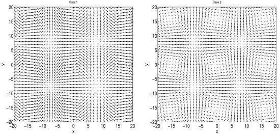
Figure 3. Snapshots of velocity fields for Model 1 (left) and Model 2 (right).

Let $S_1$ and $S_2$ be the first explosion moments for $p\left(t\right)$ and $q\left(t\right)$, respectively, then

$$S=min(S_1,S_2)$$

Certainly the knowledge of $E{S}_i$ is not enough to find $E\left(S\right)$, but the latter can be expressed in terms of $\overline{F}\left(t\right)=P\left(S_1>t\right)$ as

$$ES={\int }_0^{\infty }\overline{F}{\left(t\right)}^{2}dt$$

Manipulating with this formula it is not difficult to present an example where the expected value of the minimum of two independent identically distributed random variables $X,Y$ is finite while the expectation of each variable is infinite due to heavy tails of $X,Y$ distribution. So, theoretically speaking $E{S}_i$ and $E\left(S\right)$ may differ by an order of magnitude. Fortunately it is not the case here since the tail of distribution of $S_1$ is exponential and can be evaluated [13].

Namely from Theorem 1.1 in [13] it follows that the exponential moment

$$E\left(e^{\gamma S_1}\right)<\infty$$

(23)

is finite for all $\gamma =\gamma \left(s\right)$ satisfying

$$\gamma \left(s\right)<\frac{1}{g\left(s\right)}$$

(24)

and

$$g\left(s\right)=max\left\{x:\left({\int }_{-\infty }^{x}exp(y^3/3s^2+y^2/2s^2)dy\right)\left({\int }_x^{\infty }exp(-y^3/3s^2-y^2/2s^2)dy\right)\right\}.$$

Hence, it is reasonable to assume that

$$\overline{F}\left(t\right)\ge e^{-\gamma t}$$

(25)

with $\gamma$ satisfying (24). In view of this assumption

$$E\left(S\right)>\frac{1}{2g\left(s\right)}$$

On the other side obviously that

$$E\left(S\right)<E\left(S_1\right)$$

Thus, for the mean number of caustics $\nu \left(s\right)=1/E\left(S\right)$ one gets from (9)

$${\displaystyle {\left(2{\pi }^2\sqrt{z}M{\left(z\right)}^2\right)}^{-1}<\nu \left(s\right)<2g\left(s\right).}$$

For small s asymptotics of the lower bound and upper bound coincide and we get

$${\displaystyle \nu \left(s\right)\approx \frac{1}{4\pi s^{3/2}}{e}^{-\frac{1}{6s^2}},}$$

while for large s the corresponding asymptotics differ just by a constant

$$0.4s^{2/3}<\nu \left(s\right)<1.25s^{2/3}.$$

Approximation (25) is quite speculative and indeed it greatly overestimates $\nu \left(s\right)$. It can be seen by comparing the bounds with exact curve $\nu \left(s\right)$ obtained from solving the corresponding PDE for $\overline{F}\left(t\right)$ (Section 1). The upper and lower bounds for $\nu \left(s\right)$ are shown in Figure 4 as well as its numerical version.

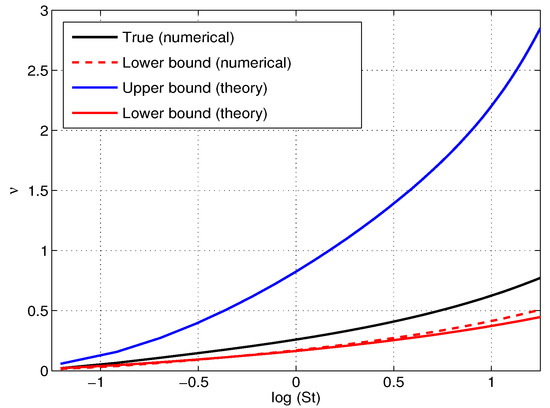
Figure 4. The theoretical upper and lower bounds for the caustic rate $\nu \left(s\right)$ as functions of Stokes number s and its numerical version.

In Model 2 LE cannot be found by such simple tools because the equations for x and y components do not split.

Finally, notice that LE in Model 1 is given by the same expression (11) as in $1D$ case. Indeed, in this case each component of the separation process $\Delta \mathbf{r}=\mathbf{r}(t,\mathbf{a})-\mathbf{r}(t,\mathbf{0})$ is the separation process for one dimensional flow (6). Hence $|\Delta \mathbf{r}|\approx \left|\mathbf{a}\right|exp\left(\lambda t\right)$ for small $\left|\mathbf{a}\right|$ and large t, where $\lambda$ is LE for (6). Then our claim follows from Definition (2).

6. Isotropic Forcing

Assume that in the original equations the forcing is isotropic, then its covariances are given by [3]

$$\begin{array}{ccc}\hfill b^{11}(x,y)& =& b_N\left(r\right)+\frac{x^2}{r^2}(b_L\left(r\right)-b_N\left(r\right)),b^{22}(x,y)=b_N\left(r\right)+\frac{y^2}{r^2}(b_L\left(r\right)-b_N\left(r\right)),\hfill \\ \hfill b^{12}(x,y)& =& b^{21}(x,y)=\frac{xy}{r^2}(b_L\left(r\right)-b_N\left(r\right)),\hfill \end{array}$$

where $r=\sqrt{x^2+y^2}$. Assume smooth longitudinal and normal correlation functions

$$\begin{array}{ccc}\hfill b_L\left(r\right)& =& b_0-\frac{1}{2}{\beta }_L{r}^2+O\left(r^4\right),\hfill \\ \hfill b_N\left(r\right)& =& b_0-\frac{1}{2}{\beta }_N{r}^2+O\left(r^4\right),\hfill \end{array}$$

with $b_0,{\beta }_L,{\beta }_N>0$. Introduce $s_L=\sqrt{2{\beta }_L{\tau }^3},s_N=\sqrt{2{\beta }_N{\tau }^3}$

Then from (17) it can be derived that (15) takes form

$$\begin{array}{ccc}d{m}_1\hfill & =\hfill & (-m_1+(m_4^2-m_1^2-m_2^2-m_3^2)/2)dt+s_{L}d{w}_1,\hfill \\ d{m}_2\hfill & =\hfill & (-m_1{m}_2-m_2)dt+s_{N}d{w}_2,\hfill \\ d{m}_3\hfill & =\hfill & (-m_1{m}_3-m_3)dt+s_{L}d{w}_3,\hfill \\ d{m}_4\hfill & =\hfill & (-m_1{m}_4-m_4)dt+s_{N}d{w}_4,\hfill \end{array}$$

here $w_j,j=1,2,3,4$ are independent standard Wiener processes.

No essential progress is made in analyzing this system yet because none of variables can be eliminated. The only reason for presenting it here is a great importance of the isotropic case for applications.

7. Conclusions and Discussion

While one dimensional stochastic models for inertial particles have been comprehensively addressed, refs. [4,6,7,9] no essential progress in analytical studies for $2D$ turbulence have been reported yet. In this work for the first time the intensity of the caustics was rigorously treated in the framework of two dimensional stochastic flows modeling $2D$ turbulence in compressible media.

Namely, we revealed two cases, where the mean time to explosion in the particle density, $\mu \left(s\right)$, can be analytically estimated for the full range of Stokes number s and can be accurately evaluated by solving an initial/boundary problem for a one dimensional parabolic equation. Worth noting that both boundaries provide an exact asymptotic as $s\to 0$. For both models the reciprocal $\nu \left(s\right)=1/\mu \left(s\right)$, interpreted as the intensity of caustics, increases monotonically from zero to infinity that is in full agreement with physics of phenomena in question.

The reported advance in the proposed models is due to reduction in the number of unknowns in the system (15) from four to two. Alas, for the most interesting isotropic case such a reduction is not possible, but a hope for finding asymptotics of $\nu \left(s\right)$ still remain. This is the main direction of our future studies.

Another interesting area of further consideration is the Equation (4) describing the Eulerian velocity field generating Lagrangian motion covered by model (1). It should be recognized that the interpretation of $\mu$ and $\nu$ in terms of solutions of (4) is not clear enough except the deterministic case with the initial velocity field ${\mathbf{u}}_0\left(\mathbf{x}\right)$ for which $|\partial {\mathbf{u}}_0/\partial \mathbf{x}|$ and $\nabla ·{\mathbf{u}}_0$ do not depend on $\mathbf{x}$ at all. A natural and important question is how the mean time until the uniqueness loss depends on the initial velocity field.

Appendix A.1. Proof of Proposition 2

The proof is based on the following statement

Lemma A1.

If there exist real m and smooth bounded function $V\left(x\right)$ such that

$$V(\infty )=V(-\infty )=0$$

(A1)

and

$$LV\left(x\right)=x-m,$$

(A2)

then with probability one

$$\overline{p}=m$$

Proof. 

From (A2) and Ito formula it follows that $V\left(p\right(t\left)\right)$ satisfies

$$dV=(p-m)dt+s{V}^{\prime }dw.$$

By integrating both sides we get

$$\frac{1}{T}(V\left(p\left(T\right)\right)-V\left(p\left(0\right)\right)=\frac{1}{T}{\int }_0^{T}p\left(t\right)dt-m+\frac{s}{T}{\int }_0^T{V}^{\prime }\left(p\left(t\right)\right)dw$$

(A3)

□

The second term on the right hand side goes to zero as $T\to \infty$ due to the large numbers law. The difference on the left hand side (LHS) of (A4) also converges to zero because of the boundness of V and condition (A1). Lemma is proven.

Notice importance of (A1). If $V(\infty )\ne V(-\infty )$ then the jumps of V at explosion moments can accumulate leading to a non-zero limit of LHS.

Now we directly construct such a function $V\left(x\right)$ and determine m.

First, we take a bounded solution of (A2)

$${\displaystyle V\left(x\right)=\frac{1}{s^2}{\int }_{-\infty }^{x}exp\left(\frac{y^3/3+y^2/2}{s^2}\right){\int }_y^{\infty }exp\left(-\frac{u^3/3+u^2/2}{s^2}\right)(u-m)dudy.}$$

for which $V(-\infty )=0$. To ensure (A1) one should set

$$m=\frac{M}{N}$$

where

$$\begin{array}{c}M={\int }_{-\infty }^{\infty }exp\left(\frac{y^3/3+y^2/2}{s^2}\right){\int }_y^{\infty }exp\left(-\frac{u^3/3+u^2/2}{s^2}\right)ududy\hfill \\ \\ N={\int }_{-\infty }^{\infty }exp\left(\frac{y^3/3+y^2/2}{s^2}\right){\int }_y^{\infty }exp\left(-\frac{u^3/3+u^2/2}{s^2}\right)dudy\hfill \end{array}$$

(A4)

The integral for M is meant as Cauchy principal value. That allows for changing the order of integration after substitution

$$t=u-y,y^{\prime }=y{s}^{2/3}$$

Integration in $y^{\prime }$ leads to

$$m=\frac{1}{2}\left(-1+\frac{g^{\prime }\left(z\right)}{2\sqrt{z}g\left(z\right)}\right)$$

where

$$g\left(z\right)={\int }_0^{\infty }exp(zt-t^3/12)\frac{dt}{\sqrt{t}}.$$

To complete the proof one should account for [11],

$$g\left(x\right)={\pi }^{-1}M{\left(x\right)}^2.$$

This relation also can be derived from the fact that the both sides satisfy the same differential equation and same initial conditions [14].

Finally, notice that the expression for m after changing the order of integration in (A4) turns to the mean of $p\left(t\right)$ with respect to the invariant measure $\pi \left(p\right)$ given in (12)

Proposition 2 is proven.

Appendix A.2. Details of the Computational Algorithm for solving (10)

Let h and $\Delta t$ be space and time, respectively, $X>0$ a big enough number, $x_i=-X+(i-1)h,n=(n-1)\Delta t$ the corresponding space/time grid, $i=1,\dots ,M,n=1,\dots ,N$ where $h=2X/M,\Delta t=t/N$. Set $b_i=\Delta t(x_i+x_i^2+s^2/h),a=\Delta t{s}^2/h$. Then a standard Eulerian scheme for (23) is written as

$$\begin{array}{c}{u}_{i+1}\left(n\right)=u_i\left(n\right)+h{y}_i\left(n\right)\hfill \\ \\ u_{i+1}(n+1)-u_{i+1}\left(n\right)=a{y}_{i+1}\left(n\right)-b_i{y}_i\left(n\right)\hfill \end{array}$$

(A5)

Notice that (A5) is well posed because $u_i\left(1\right)=1,i=1,\dots ,M,u_1\left(n\right)=0,y_M\left(n\right)=0,n=1,\dots ,N$

The choice of parameters $X,h,\Delta t$ was dictated by standard conditions on ratio $\Delta t/h$ and constraints

$$\sum _1^N\overline{F}\left(n\right)\Delta t\approx \mu \left(s\right)$$

where $\mu \left(s\right)=E\left(S\right)$ is the exact value of the expectation of S found from (9). In particular $\mu (1/\sqrt{2})$ =8.7735 while under our choice of $X=7.5,\Delta t=0.001,M=61$ it was obtained that

$$\sum _1^N\overline{F}\left(n\right)\Delta t\approx 8.7785$$

A similar comparison for other s can be seen from Figure 4.

Appendix A.3. Derivation of (15)

For the purpose of nondimensionalizing let us redenote the forcing on RHS of (14) by capital letters $W^{\left(i\right)}(t,x,y),i=1,2$. Then by differentiating (14) in a and b we get

$$\begin{array}{c}\hfill d{u}_a=-(u_a/\tau )dt+x_{a}d{\xi }_1+y_{a}d{\xi }_2,d{v}_a=-(v_a/\tau )dt+x_{a}d{\xi }_1+y_{a}d{\xi }_4,d{x}_a=u_{a}dt,d{y}_a=v_{a}dt\\ \\ \hfill d{u}_b=-(u_b/\tau )dt+x_{b}d{\xi }_1+y_{b}d{\xi }_2,d{v}_b=-(v_b/\tau )dt+x_{b}d{\xi }_1+y_{b}d{\xi }_4,d{x}_b=u_{a}dt,d{y}_b=v_{b}dt\end{array}$$

where

$${\xi }_1=\partial W^{\left(1\right)}/\partial x,{\xi }_2=\partial W^{\left(1\right)}/\partial y,{\xi }_3=\partial W^{\left(2\right)}/\partial x,{\xi }_4=\partial W^{\left(2\right)}/\partial y$$

and the covariance matrix of $\xi$’s is given by

$$\left(\begin{array}{cccc}-B_{xx}^{11}\hfill & 0& -B_{xx}^{12}\hfill & -B_{xy}^{12}\\ 0\hfill & -B_{yy}^{11}& -B_{xy}^{12}\hfill & -B_{yy}^{12}\\ -B_{xx}^{12}\hfill & -B_{xy}^{12}& -B_{xx}^{22}\hfill & 0\\ -B_{xy}^{12}\hfill & -B_{yy}^{12}& 0\hfill & -B_{yy}^{22}\end{array}\right)$$

where $B^{ij}$ is the space covariance matrix of $\left(W^{\left(1\right)},W^{\left(2\right)}\right)$

Introduce

$$\begin{array}{ccc}\hfill J_1\left(t\right)& \equiv & \frac{\partial x}{\partial a}\frac{\partial v}{\partial b}-\frac{\partial x}{\partial b}\frac{\partial v}{\partial a},\hfill \\ \hfill J_2\left(t\right)& \equiv & \frac{\partial y}{\partial a}\frac{\partial u}{\partial b}-\frac{\partial y}{\partial b}\frac{\partial u}{\partial a},\hfill \\ \hfill J_3\left(t\right)& \equiv & \frac{\partial x}{\partial a}\frac{\partial u}{\partial b}-\frac{\partial x}{\partial b}\frac{\partial u}{\partial a},\hfill \\ \hfill J_4\left(t\right)& \equiv & \frac{\partial y}{\partial a}\frac{\partial v}{\partial b}-\frac{\partial y}{\partial b}\frac{\partial v}{\partial a},\hfill \\ \hfill J_5\left(t\right)& \equiv & \frac{\partial u}{\partial a}\frac{\partial v}{\partial b}-\frac{\partial u}{\partial b}\frac{\partial v}{\partial a},\hfill \end{array}$$

Applying Ito formula we obtain

$$\begin{array}{ccc}\hfill dJ& =& (J_1-J_2)dt,\hfill \\ \hfill d{J}_1& =& (-J_1/\tau +J_5)dt+Jd{\xi }_4,\hfill \\ \hfill d{J}_2& =& (-J_2/\tau -J5)dt+Jd{\xi }_1,\hfill \\ \hfill d{J}_3& =& (-J_3/\tau )dt+Jd{\xi }_2,\hfill \\ \hfill d{J}_4& =& (-J_4/\tau )dt+Jd{\xi }_3,\hfill \\ \hfill d{J}_5& =& (-J_5/\tau )dt+J_{1}d{\xi }_1+J_{2}d{\xi }_2-J_{3}d{\xi }_3-J_{4}d{\xi }_4,\hfill \end{array}$$

To proceed to dimensionless variables assume

$$W^{\left(i\right)}(t,x,y)=\sigma {\tau }^{1/2}{w}^{\left(i\right)}(t/\tau ,x/L,y/L),i=1,2$$

where $w^{\left(i\right)}$ are dimensionless Wiener processes, thereby in dimensionless variables

$$Ed{w}^{\left(i\right)}(t,0,0)d{w}^{\left(j\right)}(t,x,y)=b^{ij}(x,y)dt$$

with

$$B^{ij}(x,y)={\sigma }^2{b}^{ij}(x/L,y/L)$$

Introduce a Stokes number similarly to (8)

$$s=\sigma {\tau }^{3/2}/L$$

The result is

$$\begin{array}{ccc}dJ\hfill & =\hfill & I_{1}dt,\hfill \\ d{I}_1\hfill & =\hfill & (-I_1+2J_5)dt+sJd{\eta }_1,\hfill \\ d{I}_2\hfill & =\hfill & -I_{2}dt+sJd{\eta }_2,\hfill \\ d{I}_3\hfill & =\hfill & -I_{3}dt+sJd{\eta }_3,\hfill \\ d{I}_4\hfill & =\hfill & -I_{4}dt+sJd{\eta }_4\hfill \end{array}$$

$$I_1=\tau (J_1-J_2),I_2=\tau (J_1+J_2),I_3=\tau (J_4-J_3),I_4=\tau (J_3+J_4)$$

where

$${\eta }_1=({\xi }_4-{\xi }_1)/h,{\eta }_2=({\xi }_4+{\xi }_1)/h,{\eta }_3=({\xi }_3-{\xi }_2)/h,{\eta }_4=({\xi }_3+{\xi }_2)/h,h=\sigma {\tau }^{1/2}$$

We do not need a stochastic equation for $J_5$ since it can be found from the following equation

$$I_2^2-I_1^2-I_4^2+I_3^2=-4J{J}_5,$$

(A6)

which follows from

$$J_1{J}_2+J{J}_5=J_3{J}_4.$$

We can reduce the number of freedom degrees by introducing $m_k=I_k/J,k=1,\dots ,4$ and eliminating $J_5$ by means of (A6). The result is system (15).

References

- Kunita, H. Stochastic Flows and Stochastic Differential Equations; Cambridge University Press: Cambridge, UK, 1990. [Google Scholar]
- Piterbarg, L.I. The top Lyapunov exponent for a stochastic flow modeling the upper ocean turbulence. SIAM J. Appl. Math. 2001, 62, 777–800. [Google Scholar] [CrossRef]
- Monin, A.S.; Yaglom, A.M. Statistical Fluid Mechanics: Mechanics of Turbulence; MIT Press: Cambridge, MA, USA, 1975. [Google Scholar]
- Gustavsson, K.; Mehlig, B. Statistical models for spatial patterns of inertial particles in turbulence. arXiv 2014, arXiv:1412.4374v1. [Google Scholar]
- Meibohm, J. On the Phase-Space Distribution of Heavy Particles in Turbulence. Ph.D. Thesis, University of Gothenburg, Göteborg, Sweden, 3 January 2020. [Google Scholar]
- Falkovich, G.; Musacchio, S.; Piterbarg, L.; Vucelja, M. Inertial particles driven by a telegraph noise. Phys. Rev. E 2007, 76, 026313. [Google Scholar] [CrossRef] [PubMed]
- Horvai, P. Lyapunov exponent for inertial particles in the 2D Kraichnan model as a problem of Anderson localization with complex valued potential. arXiv 2005, arXiv:nlin/0511023. [Google Scholar]
- Boffetta, G.; Ecke, R.E. Two-dimensional turbulence. Annu. Rev. Fluid Mech. 2012, 44, 427–451. [Google Scholar] [CrossRef]
- Mehlig, B.; Wilkinson, M. Coagulation by random velocity fields as a Kramers problem. Phys. Rev. Lett. 2004, 92, 250602. [Google Scholar] [CrossRef] [PubMed]
- Karatzas, I.; Shreve, S.E. Brownian Motion and Stochastic Calculus; Springer: Berlin/Heidelberg, Germany, 1991. [Google Scholar]
- Halperin, B.I. Green’s functions for a particle in a one-dimensional random potential. Phys. Rev. 1965, 139, A104–A117. [Google Scholar] [CrossRef]
- Karatzas, I.I.; Shreve, S.E. Distribution of the time to explosion for one-dimensional diffusions. Probab. Theory Relat. Fields 2016, 164, 1027–1069. [Google Scholar] [CrossRef]
- Loukianov, O.; Loukianova, D.; Song, S. Spectral gaps and exponential integrability of hitting times for linear diffusions. Ann. Inst. Henri Poincaré Probab. Statist. 2011, 47, 679–698. [Google Scholar] [CrossRef]
- Abramowitz, M.; Stegun, I.A. Handbook of Mathematical Functions; Dover Publications, INC.: New York, NY, USA, 1970. [Google Scholar]
Publisher’s Note: MDPI stays neutral with regard to jurisdictional claims in published maps and institutional affiliations. |
© 2021 by the author. Licensee MDPI, Basel, Switzerland. This article is an open access article distributed under the terms and conditions of the Creative Commons Attribution (CC BY) license (https://creativecommons.org/licenses/by/4.0/).