Generalization of Methods for Calculating Steady-State Flow Distribution in Pipeline Networks for Non-Conventional Flow Models

Abstract

This paper proposes generalized models and methods for calculating flow distribution in hydraulic circuits with lumped parameters. The main models of the isothermal steady-state flow of medium are classified by an element of the hydraulic circuit. These models include conventional, implicitly specified by flow rate, and pressure-dependent ones. The conditions for their applicability, which ensure the existence and uniqueness of a solution to the flow distribution problem, are considered. We propose generalized nodal pressure and loop flow rate methods, which can be applied regardless of the forms of specific element models. Final algorithms, which require lower computational costs versus the known approaches designed for non-conventional flow models, are substantiated. Proposed models, methods, algorithms, and their capabilities, are analytically and numerically illustrated by an example of a fragment of gas transmission network with compressor stations.

1. Introduction

The problems of flow distribution are the fundamental problems of analysis and justification of decisions on the management of operation modes of pipeline systems (PLSs) of various types and purposes (heat-, water-, oil-, gas supply, etc.) in their design, operation, and supervisory control. The requirements for the efficiency of the methods of solving these problems are constantly increasing. Such requirements include the following: (1) speed; (2) reliability, which manifests itself in the guaranteed solutions with a predetermined accuracy; (3) ability to solve high-dimensional problems; (4) universality with respect to an arbitrary structure of the object of the analysis, the composition of its elements, and changes in design conditions.

The expediency of development and elaboration of unified methods for modeling operation modes of PLSs of various types is due to the commonality of the following: (1) their structural and topological properties; (2) physical laws of liquid (gas) flow in individual elements; (3) conservation laws of networks; (4) conceptual and mathematical statements of analysis problems. Therefore, in what follows, when considering models and methods, we will use the term “hydraulic circuit” (HC), irrespective of the specific purpose of the PLSs being modeled.

The conventional model of steady-state isothermal flow distribution in the HC with concentrated parameters includes Kirchhoff laws and closing relations. It represents a system of linear and nonlinear algebraic equations, and there are two basic forms of writing such models: the nodal and loop ones. The nodal model is as follows [1,2]:

$$Ax=Q,{\overline{A}}^T\overline{P}=y,y=f(x),$$

(1)

where $\overline{A}$—a complete $(m\times n)$-matrix of incidences of nodes and branches of the directed graph of the analytical circuit model with elements of $a_{ji}=1\left(-1\right)$, if node $j$ is initial (final) one for branch $i$ and $a_{ji}=0$, if branch $i$ is not incident to node $j$; $x,y$—$n$-dimensional vectors of flow rates and pressure drops at the branches of the analytical circuit model; $A$—a $[(m-1)\times n]$-matrix of incidences formed from $\overline{A}$ by crossing out one of the linearly dependent lines; $f\left(x\right)$—a $n$-dimensional vector-function with elements $f_i\left(x_i\right),i=\overline{1,n}$, reflecting the laws of the pressure drop as a function of flow rate (flow model) at the branches of the HC; $Q$—a ($m-1$)-dimensional vector of nodal flow rates with elements $Q_j>0$ ($Q_j<0$) if node $j$ has an inflow (extraction) and $Q_j=0$, if node $j$ is a simple branch connection point; $\overline{P}$—a $m$-dimensional vector of nodal pressures.

The loop model differs only in the way the second Kirchhoff law is written: instead of the second relation in (1) one uses $By=0$. Here ($B$) is a ($c\times n$)-matrix of loops, with elements $b_{ri}=1\left(-1\right)$, if the orientation of branch $i$ coincides (does not coincide) with the direction of traversal of loop $r$ and $b_{ri}=0$, if branch $i$ is not included in loop $r$; $c$ is the number of main loops equal to the number of branches of the HC not included in the spanning tree of the HC, and called chords. Hence $c=n-m+1$. The equivalence of both forms of notation follows from the fact that $B({\overline{A}}^T\overline{P}=y)\Rightarrow 0=By$ due to the well-known property of orthogonality of matrices $A$ and $B$ [3].

Let $\overline{P}=\left[\begin{array}{c}P\\ P_m\end{array}\right]$, then the classical problem of flow distribution consists in determining vectors $x,y$ and $P$ given the known form of $f_i\left(x_i\right)$, $i=\overline{1,n}$, predetermined matrix $\overline{A}$, vector $Q$, and pressure at one of the nodes ($P_m$), which for simplicity’s sake is assumed to be zero. In the loop model, vector $P$ is determined after solving the problem with respect to $x$ and $y$.

Numerous methods and algorithms for solving this problem are known, an overview of which can be found, for example, in [1,4], etc. However, the main ones are the classical methods: those of node and loop methods (NM and LM) [1,2,5,6,7,8], etc., which have been widely adopted in modeling the operation modes of PLSs of heat- [1,9,10], etc., water- [1,9], etc., gas supply [11,12,13], etc.

Both methods are based on the Newton-Raphson method in conjunction with special methods of decreasing the order of the system of linearized equations to be solved. Let us introduce decomposition $x=\left[\begin{array}{c}{x}_C\\ x_T\end{array}\right]$, where $x_C,x_T$ are the flow rate vectors at the chords and branches of the spanning tree, respectively. Finding the direction of the Newton-Raphson decrement to the flow rates at the chords ($\mathsf{\Delta }{x}_C^k$) in the LM and to the nodal pressures ($\mathsf{\Delta }{P}^k$) in the NM at the $k$-th iteration involves solving the following systems of equations:

$$B{f^{\prime }}_x{B}^T\mathsf{\Delta }{x}_L^k=-Bf(x^k),$$

(2)

$$A{({f^{\prime }}_x)}^{-1}{A}^T\mathsf{\Delta }{P}^k=Q-A{\mathrm{x}}^k,$$

(3)

where ${f^{\prime }}_x=\frac{\partial f}{\partial x}$ is the diagonal matrix of partial derivatives at point $x^k$.

In both systems the coefficient matrices are symmetric. For two-dimensional circuits (which is typical of most real-life PLSs), matrix (2) of coefficients of the system has a strict diagonal predominance, and in (3) it is not strict. Therefore, the LM usually requires fewer iterations than the NM (although the situation is corrected if one applies a decrement length adjustment to the NM). Computational costs are also related to the order of systems to be solved, which are different in these methods ($c$ in (2) and $m-1$ in (3)). Figure 1 shows limiting examples of analytical circuit models illustrating the absolute dominance of the LM for the circuit in Figure 1a and that of the NM for the circuit in Figure 1b, since in this case each of systems (2) and (3) is reduced to a single equation. But these systems can be arbitrarily large if one applies the LM to the circuit in Figure 1b, and the NM to the circuit in Figure 1a. Therefore, in general, both methods have their place and the areas of applications where one of them proves more preferable than the other.

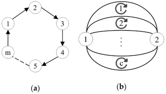
Figure 1. Examples of analytical circuit models where one of the methods is deemed more preferable than the other: (a) LM; (b) NM.

Analysis of numerous dependencies and formulas for the description of the steady isothermal flow of the working fluid (liquid or gas) through pipelines and other elements of the PLS allows one to introduce the following classification as derived from the standpoint of their mathematical features [14]: (1) conventional (explicit); (2) implicit flow rate-based; (3) pressure-dependent flow models; (4) 2-and-3 hybrid cases.

In the conventional case $f_i\left(x_i\right)=s_i{x}_i|x_i|-Y_i$, where $s_i$ is the hydraulic loss of the branch, $Y_i>0$ is the pressure increment at active branches (e.g., with pumping stations) and $Y_i=0$ at passive branches (e.g., for pipeline sections). Here we have explicit expressions for derivative $\partial f_i/\partial x_i=2s_i|x_i|$ and function ${\psi }_i(y_i)=\sqrt{|y_i+Y_i|/s_i}\cdot \mathrm{sign}(y_i+Y_i)$ inverse to $f_i\left(x_i\right)$.

Implicit flow rate-based models of the flow are mainly applicable to pipelines. It follows from the basic Darcy-Weisbach formula [15] $h=\mathit{\lambda }\frac{l}{d}\frac{V^2}{2g}$ that $s=\mathit{\lambda }\frac{8l}{\rho {\pi }^2{d}_{}^5}$, since $V=4\left|x\right|/(\pi d_{}^2\rho )$ and $y=\rho gh$. Here: $h,V$—head loss (m) and flow velocity; $y,x$—pressure loss and mass flow rate of the working fluid; $l,d$—pipe length and inside diameter; $\rho$—density of the transported fluid; $g$—gravitational acceleration. The coefficient of friction drag $\mathit{\lambda }$ can be treated as a constant only in the region of fully-developed turbulence, while in the general case it depends on velocity (Reynolds number) $\mathrm{Re}(V)=Vd/\nu$, where $\nu$ is the kinematic viscosity coefficient of the fluid. Examples of such dependencies are the common Colebrook-White [16]

$$\mathit{\lambda }={\left[-2\lg \left(\frac{{\mathsf{\Delta }}_r}{3.7d}+\frac{2.51}{\mathrm{Re}\left(V\right)\sqrt{\mathit{\lambda }}}\right)\right]}^{-2}$$

and Altshul [17]

$$\mathit{\lambda }=0.11{\left(\frac{{\mathsf{\Delta }}_r}{d}+\frac{68}{\mathrm{Re}\left(V\right)}\right)}^{0.25}$$

formulas. Therefore, friction loss $s_i$ for the branch that models the pipeline will generally be a function of $s_i(x_i)$. Function ${\psi }_i(y_i)$ becomes implicit, and the derivatives required for the LM or NM to be applied must already be determined by the rules of differentiation of such functions, which produces [14]:

$${f^{\prime }}_{x,i}=\frac{d{f}_i}{d{x}_i}=(2s_i+{s^{\prime }}_{x,i}{x}_i)|x_i|,$$

where ${s^{\prime }}_{x,i}=\frac{d{s}_i}{d{x}_i}=\frac{d{s}_i}{d{\mathit{\lambda }}_i}\frac{d{\mathit{\lambda }}_i}{d{V}_i}\frac{d{V}_i}{d{x}_i}$, $\frac{d{s}_i}{d{\mathit{\lambda }}_i}=\frac{8l_i}{\rho {\pi }^2{d}_i^5}$, $\frac{d{V}_i}{d{x}_i}=\frac{4}{\pi d_i^2\rho }$.

Pressure-dependent flow models mainly arise from the working fluid (natural gas, water vapor, etc.) compressibility effect. Here the pressure loss depends not only on the flow rate but also on the value of the pressure itself. Let us give examples of such models, denoting by $p_{\mathrm{H}}$, $p_{\mathrm{K}}$ the pressures of the working fluid at the beginning and at the end of the modeled PLS element.

The dependency of the pressure built up by a centrifugal gas compressor unit on its inlet volumetric flow rate ($q_{\mathrm{H}}$) is represented as a graphical characteristic of the compression ratio $\frac{p_{\mathrm{K}}}{p_{\mathrm{H}}}=\epsilon (q_{\mathrm{H}})$. Functions $\epsilon (q_{\mathrm{H}})$ are approximated with sufficient accuracy by algebraic polynomials of degree three or lower [18,19] $\epsilon (q)=a_0+a_1{q}_{\mathrm{H}}+a_2{q}_{\mathrm{H}}^2+a_3{q}_{\mathrm{H}}^3$. Taking into account that $q=x/\rho$ and the equation of state of the gas can be represented as $\rho =p/k$ (where $k=ZRT$ is a known coefficient for a given gas temperature $T$ and its physical properties: gas constant R and compressibility coefficient Z) we arrive at the following flow model

$$\frac{p_{\mathrm{K}}}{p_{\mathrm{H}}}={\alpha }_0+\frac{{\alpha }_1}{p_{\mathrm{H}}}x+\frac{{\alpha }_2}{p_{\mathrm{H}}^2}{x}^2+\frac{{\alpha }_3}{p_{\mathrm{H}}^3}{x}^3\mathrm{or}{p}_{\mathrm{K}}=p_{\mathrm{H}}{\alpha }_0+{\alpha }_{1}x+\frac{{\alpha }_2}{p_{\mathrm{H}}^{}}{x}^2+\frac{{\alpha }_3}{p_{\mathrm{H}}^{}}{x}^3.$$

(4)

Numerous variations of this model are known [20,21], etc., they are introduced as a result of neglecting some of the terms of the polynomial or approximating ${\epsilon }^2(q_{\mathrm{H}})$ instead of $\epsilon (q_{\mathrm{H}})$.

In [22], the authors present a gas pipeline section model that allows factoring in more adequately the difference in geodetic heights of its ends

$$p_{\mathrm{H}}^2-p_{\mathrm{K}}^2=sx|x|+\frac{g\cdot l\cdot \sin (\theta )\cdot {(p_{\mathrm{H}}^{}+p_{\mathrm{K}}^{})}^2}{2\cdot k},$$

(5)

where $\theta$—pipe angle; Z—compressibility factor; R—gas constant; T—average gas temperature. In [23] an alternative model is given

$$p_{\mathrm{H}}^2-e^{\alpha }{p}_{\mathrm{K}}^2=sx|x|,$$

(6)

where $\alpha$ is the coefficient that depends on the difference of geodetic heights of the ends of the section.

When modeling the pipelines of water-steam circuits of steam-turbine plants, the following formula is used to calculate the pressure drop [24,25]

$$y=\mathit{\lambda }\frac{l}{2d\rho {\left(\tilde{p}\right)}^{\prime }{\omega }^2}\left(1+\sigma \left(\tilde{p},x\right)\cdot \chi \left(\tilde{p},x\right)\cdot \left(\frac{\rho {\left(\tilde{p}\right)}^{\prime }}{\rho {\left(\tilde{p}\right)}^{″}}-1\right)\right)x^2,$$

(7)

where $\rho {\left(\tilde{p}\right)}^{\prime }$, $\rho {\left(\tilde{p}\right)}^{″}$—densities of liquid and vapor phases of the flow in the function of average pressure $\tilde{p}$; $\omega$—cross-sectional area of the pipe; $\sigma$—coefficient that accounts for the effect of the structure of the steam-water flow on the friction loss; $\chi$—mass vapor content of the flow.

For turbine control valves the following formula applies [26]

$$1.09 p_{\mathrm{K}}{p}_{\mathrm{H}}-0.09 p_{\mathrm{H}}^2-p_{\mathrm{K}}^2=s{x}^2.$$

(8)

The above examples (4)–(8) attest to the impossibility of reducing it to conventional form $y=f(x)$, where $y=p_{\mathrm{H}}-p_{\mathrm{K}}$. Conceivably, the technique of double iteration cycles [1,2] is applicable to the analysis of the HC with such flow models. Here, in the inner iteration cycle, the classical flow-distribution problem is solved (by means of the LM or NM) at fixed values ${\tilde{s}}^{*},{\tilde{Y}}^{*}$ of pressure-dependent functions $\tilde{s}(p_{\mathrm{H}},p_{\mathrm{K}},x)$, $\tilde{Y}(p_{\mathrm{H}},p_{\mathrm{K}},x)$ of flow models $y={\tilde{s}}^{*}x|x|-{\tilde{Y}}^{*}$, and in the outer cycle, the values of these functions are defined more precisely depending on the obtained values of flow rates and pressures. For example, in (5) one can assume

$$y=p_{\mathrm{H}}^2-p_{\mathrm{K}}^2,{\tilde{Y}}^{*}=-\frac{g\cdot l\cdot \sin (\theta )\cdot {(p_{\mathrm{H}}^{*}+p_{\mathrm{K}}^{*})}^2}{2\cdot Z\cdot R\cdot T},$$

in (6) ${\tilde{Y}}^{*}=(1-e^{\alpha }){(p_{\mathrm{K}}^{*})}^2$, etc. The technique is sufficiently universal, but its application is associated with the ambiguity of arriving at functions $\tilde{s},\tilde{Y}$, the need for special justification and ensuring convergence, a multiple increase in computational costs if compared to the conventional case.

The above analysis of the published research shows that many authors: (1) pay attention to the fundamental difference of the models of the flow of compressible fluid from that of the case of incompressible fluid [12,21,22,25,27,28,29]; (2) note the impossibility or significant difficulties of applying conventional methods of analysis of the flow distribution in these cases [12,21,22,23,25,27,28,29,30,31]; (3) state the lack of general, universal methods [12,21,22,25,28,30]; (4) propose their own methods and algorithms for calculating the flow distribution in complex systems of conveying gas through trunk pipelines [12,21,22,28,29,30,31], heat and steam supply systems [25], process pipelines systems [27] and other PLSs, transporting gases or gas-liquid mixtures. The methods proposed in the published research boil down either to the technique of double iteration cycles [25,27,28], or presuppose increasing the dimensionality of the systems of equations to be solved as compared to (2) or (3) [22,23,30]. So, for example, at each step of the solution of the flow-distribution problem by the Newton-Raphson method in [12,21,22,23], etc., it is proposed to solve a system of linearized equations of order $n+m-1$ to simultaneously find the step direction by flow rates ($x$) and pressures ($P$), and in [30] it is proposed to solve that of order $n$ by flow rates ($x$).

A new method, called the modified node method (MNM), was proposed in the study [14]. It provides a solution to the problem with arbitrary flow models in the space of vector $P$. That is, at each step of the iterative process linear systems of equations of order $m$ are solved. Below, for the first time, an attempt is made to generalize the problems and methods of calculating the steady-state isothermal flow distribution in hydraulic circuits for arbitrary models of the fluid flow. In particular, a new (modified) loop method (MLM) is proposed, which provides a solution to the problem in the space of loop flow rates ($x_C$) of the order of $c$.

2. Generalization of the Flow Distribution Model and the Node Method

All of the above types of liquid or gas flow models along the elements of the HC can be reduced to a general form of writing down pressure-dependent model $\phi (p_{\mathrm{H}},p_{\mathrm{K}},x)=0$. With this in mind, instead of (1), the following generalized model of flow distribution is proposed [14]

$$Ax=Q,$$

(9)

$$p_{\mathrm{H}}=A_{\mathrm{H}}^{T}P,$$

(10)

$$p_{\mathrm{K}}=-A_{\mathrm{K}}^{T}P,$$

(11)

$$\phi (p_{\mathrm{H}},p_{\mathrm{K}},x)=0,$$

(12)

where $p_{\mathrm{H}},p_{\mathrm{K}}$—$n$-dimensional vectors of pressures at the beginning and end of branches, respectively, $A_{\mathrm{H}},A_{\mathrm{K}}$—$(m\times n)$-matrices of incidences that capture separately the initial and final nodes of branches so that $A_{\mathrm{H}}+A_{\mathrm{K}}=\overline{A}$, $\phi (p_{\mathrm{H}},p_{\mathrm{K}},x)$—a vector-function with elements ${\phi }_i(p_{\mathrm{H},i},p_{\mathrm{K},i},x_i)$, $i=\overline{1,n}$, reflecting arbitrary flow laws, including conventional ones, implicitly determined by flow and pressure-dependent.

Here are the main provisions of MNM for solving the problem of flow distribution based on model (9)–(12). Let at the k-th iteration there be value $P^k$, to which we can map unequivocal values of $p_{\mathrm{H}}^k$, $p_{\mathrm{K}}^k$ and $x^k$ from (10), (11), and (12), respectively. Linearization of Equations (9)–(12) yields

$$A\mathsf{\Delta }{x}^k=-u_1^k,$$

(13)

$$\mathsf{\Delta }{p}_{\mathrm{H}}^k=A_{\mathrm{H}}^T\mathsf{\Delta }{P}^k,\mathsf{\Delta }{p}_{\mathrm{K}}^k=-A_{\mathrm{K}}^T\mathsf{\Delta }{P}^k,$$

(14)

$${{\phi }^{\prime }}_{\mathrm{P}\mathrm{H}}\mathsf{\Delta }{p}_{\mathrm{H}}^k+{{\phi }^{\prime }}_{\mathrm{P}\mathrm{K}}\mathsf{\Delta }{p}_{\mathrm{K}}^k+{{\phi }^{\prime }}_x\mathsf{\Delta }{x}^k=0,$$

(15)

where $u_1^k=A{x}^k-Q$, and ${{\phi }^{\prime }}_{\mathrm{PH}}=\frac{\partial \phi }{\partial p_{\mathrm{H}}}$, ${{\phi }^{\prime }}_{\mathrm{P}\mathrm{K}}=\frac{\partial \phi }{\partial p_{\mathrm{K}}}$, ${{\phi }^{\prime }}_x=\frac{\partial \phi }{\partial x}$ —diagonal matrices of partial derivative matrices of order $n$. Let us express $\mathsf{\Delta }{x}^k$ from (15)— $\mathsf{\Delta }{x}^k=-{({{\phi }^{\prime }}_x)}^{-1}({{\phi }^{\prime }}_{\mathrm{P}\mathrm{H}}\mathsf{\Delta }{p}_{\mathrm{H}}^k+{{\phi }^{\prime }}_{\mathrm{P}\mathrm{K}}\mathsf{\Delta }{p}_{\mathrm{K}}^k)$. Given (14) we obtain

$$\mathsf{\Delta }{x}^k=-{({{\phi }^{\prime }}_x)}^{-1}({{\phi }^{\prime }}_{\mathrm{P}\mathrm{H}}{A}_{\mathrm{H}}^T-{{\phi }^{\prime }}_{\mathrm{P}\mathrm{K}}{A}_{\mathrm{K}}^T)\mathsf{\Delta }{P}^k.$$

(16)

Substituing (16) in (13) yields

$$A{({{\phi }^{\prime }}_x)}^{-1}\left({{\phi }^{\prime }}_{\mathrm{P}\mathrm{H}}{A}_{\mathrm{H}}^T-{{\phi }^{\prime }}_{\mathrm{P}\mathrm{K}}{A}_{\mathrm{K}}^T\right)\mathsf{\Delta }{P}^k=u_1^k.$$

(17)

By the rules of differentiation of implicit functions

$${({x^{\prime }}_{\mathrm{P}\mathrm{H}})}_i=\frac{\partial x_i}{\partial p_{\mathrm{H}i}}=-{\left(\frac{\partial {\phi }_i}{\partial x_i}\right)}^{-1}\frac{\partial {\phi }_i}{\partial p_{\mathrm{H}i}}\mathrm{and}{({x^{\prime }}_{\mathrm{PK}})}_i=\frac{\partial x_i}{\partial p_{\mathrm{K}i}}=-{\left(\frac{\partial {\phi }_i}{\partial x_i}\right)}^{-1}\frac{\partial {\phi }_i}{\partial p_{\mathrm{K}i}},i=\overline{1,n}.$$

Hence, ${x^{\prime }}_{\mathrm{P}\mathrm{H}}=-{({{\phi }^{\prime }}_x)}^{-1}{{\phi }^{\prime }}_{\mathrm{P}\mathrm{H}}$, ${x^{\prime }}_{\mathrm{P}\mathrm{K}}=-{({{\phi }^{\prime }}_x)}^{-1}{{\phi }^{\prime }}_{\mathrm{P}\mathrm{K}}$ and are the diagonal matrices of the corresponding partial derivatives of order $n$. Then system (17) can be represented as

$$[A{({x^{\prime }}_{\mathrm{P}\mathrm{H}})}^k{A}_{\mathrm{H}}^T-A{({x^{\prime }}_{\mathrm{P}\mathrm{K}})}^k{A}_{\mathrm{K}}^T]\mathsf{\Delta }{P}^k=-u_1^k.$$

(18)

Thus, the proposed MNM is reduced to an iterative process of finding a solution in the space of nodal pressures $P^{k+1}=P^k+{\mathit{\lambda }}^k\mathsf{\Delta }{P}^k$, where $\mathsf{\Delta }{P}^k$ is determined based on the solution of (18), ${\mathit{\lambda }}^k$—step length as determined by the condition of one-dimensional minimization of some norm of vector $u_1^k$.

We will also show that the considered NM modification covers the canonical case when

$$\phi (p_{\mathrm{H}},p_{\mathrm{K}},x)=p_{\mathrm{H}}-p_{\mathrm{K}}-f(x)=0.$$

(19)

In this case ${{\phi }^{\prime }}_{\mathrm{P}\mathrm{H}}=E_n$, ${{\phi }^{\prime }}_{\mathrm{P}\mathrm{K}}=-E_n$, where $E_n$ is a unit matrix of order $n$, and

$$\left({{\phi }^{\prime }}_{\mathrm{P}\mathrm{H}}{A}_{\mathrm{H}}^T-{{\phi }^{\prime }}_{\mathrm{P}\mathrm{K}}{A}_{\mathrm{K}}^T\right)=\left(E_n{A}_{\mathrm{H}}^T+E_n{A}_{\mathrm{K}}^T\right)=A_{\mathrm{H}}^T+A_{\mathrm{K}}^T=A^T.$$

Given that ${{\phi }^{\prime }}_x=-{f^{\prime }}_x$, instead of (17) we have (3).

This section may be divided by subheadings. It should provide a concise and precise description of the experimental results, their interpretation as well as the experimental conclusions that can be drawn.

3. Conditions of Existence and Uniqueness of the Solution

Proofs of the existence and uniqueness of the solution to the conventional problem of flow distribution as based on model (1) are given in [1,32,33]. The existence and uniqueness conditions are reduced to the requirement of monotonicity of functions $f_i(x_i),i=\overline{1,n}$. Namely, these functions must be smooth (continuously differentiable) and monotonically increasing, i.e., $f_i(x_i^{**})>f_i(x_i^{*})$ given $x_i^{**}>x_i^{*}$ (Figure 2a). For the conventional model represented in the generalized form (19), these conditions are equivalent to simultaneously meeting requirements of monotone increasing ${\phi }_i(p_{\mathrm{H},i},x_i)$ (for arbitrary fixed $p_{\mathrm{K},i}^{*}$) and monotone decreasing ${\phi }_i(p_{\mathrm{K},i},x_i)$ (for fixed $p_{\mathrm{H},i}^{*}$) over the entire set of values $p_{\mathrm{H},i}^{},p_{\mathrm{K},i},x_i$ (Figure 2b,c). Therefore, the requirements for monotonicity of ${\phi }_i(p_{\mathrm{H},i},p_{\mathrm{K},i},x_i)$, $i=\overline{1,n}$, can be formulated as

$$\frac{\partial p_{\mathrm{H},i}}{\partial x_i}=-{\left(\frac{\partial {\phi }_i}{\partial p_{\mathrm{H}i}}\right)}^{-1}\frac{\partial {\phi }_i}{\partial x_i}>0,\frac{\partial p_{\mathrm{K}i}}{\partial x_i}=-{\left(\frac{\partial {\phi }_i}{\partial p_{\mathrm{K}i}}\right)}^{-1}\frac{\partial {\phi }_i}{\partial x_i}<0,i=\overline{1,n}.$$

(20)

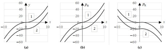
Figure 2. Charts of conventional flow models for the passive (1) and active (2) branches of the HC in coordinates: (a) $(x,y)$; (b) $(p_{\mathrm{H}},x)$; (c) $(p_{\mathrm{K}},x)$.

Let us consider the properties of coefficient matrix (18)

$$\tilde{M}=A{({x^{\prime }}_{\mathrm{P}\mathrm{H}})}^k{A}_{\mathrm{H}}^T-A{({x^{\prime }}_{\mathrm{P}\mathrm{K}})}^k{A}_{\mathrm{K}}^T,$$

first denoting ${\tilde{\eta }}_i={\left(x_{\mathrm{PH}}^{\prime }\right)}_i, {\tilde{\kappa }}_i={\left(x_{\mathrm{PK}}^{\prime }\right)}_i, i=\overline{1,n}$. Diagonal elements $\tilde{M}$ are defined as ${\tilde{M}}_{jj}={\displaystyle \sum _{i\in I_j^{-}}{\tilde{\eta }}_i}-{\displaystyle \sum _{i\in I_j^{+}}{\tilde{\kappa }}_i}$, where $I_j^{-}$($I_j^{+}$) is the set of branches coming from (going into) node $j$. Off-diagonal elements: ${\tilde{M}}_{jt}=0$, if nodes $j$ and $t$ are not connected by any branches; ${\tilde{M}}_{jt}={\tilde{\kappa }}_i$, if nodes $j$ and $t$ are connected by single branch $i$ and $t$ is its terminal node; ${\tilde{M}}_{jt}=-{\eta }_i$, when $t$ is the initial node of branch $i$; ${\tilde{M}}_{jt}=-{\displaystyle \sum _{i\in I_{jt}}{\tilde{\eta }}_i}+{\displaystyle \sum _{i\in I_{jt}}{\tilde{\kappa }}_i}$, if nodes $j$ and $t$ are connected by parallel branches that form set $I_{jt}$. If conditions ${\left(x_{\mathrm{PH}}^{\prime }\right)}_i>0, {\left(x_{\mathrm{PK}}^{\prime }\right)}_i<0, i=\overline{1,n}$ are met, being equivalent to (20), we have ${\tilde{\eta }}_i>0, {\tilde{\kappa }}_i<0, i=\overline{1,n}$. Hence ${\tilde{M}}_{jt}>0$ given $j=t$ and ${\tilde{M}}_{jt}\le 0$ given $j\ne t$ for all $j,t=\overline{1,m-1}$. In this case, ${\tilde{M}}_{jj}\ge {\displaystyle \sum _{t=1,t\ne j}^{m-1}\left|{\tilde{M}}_{jt}\right|},j=\overline{1,m-1}$, where there is a strict inequality when node $j$ (or $t$) is incidental to a branch that has node $m$ with a given pressure at the other end. Thus (as in the classical case (3)) $\tilde{M}$ has a non-strict diagonal predominance, is symmetric in structure, although is not symmetric in the values of its components. These circumstances, combined with step length adjustments, allow for confident convergence of the MNM [14].

4. Generalized Loop Flow Rates Method

To justify the method of solving the problem in the space of loop flow rates, let us introduce the following notations for the equations of model (9)–(12)

$$u_1(x)=\overline{A}x-Q=0,$$

(21)

$$u_2(p_{\mathrm{H}},P)=p_{\mathrm{H}}-A_{\mathrm{H}}^{T}P=0,$$

(22)

$$u_3(p_{\mathrm{K}},P)=p_{\mathrm{K}}+A_{\mathrm{K}}^{T}P=0,$$

(23)

$$\phi (p_{\mathrm{H}},p_{\mathrm{K}},x)=0.$$

(24)

Let there be a k-th approximation to the solution such that $u_1^k=0$, $u_2^k=0$, $u_3^k=0$, ${\phi }^k=\phi (p_{\mathrm{H}}^k,p_{\mathrm{K}}^k,x^k)$, ${\phi }_T^k=0$. The linearization of Equations (21)–(24) at the point of this approximation yields

$$\overline{A}\mathsf{\Delta }{x}^k=0,$$

(25)

$$\mathsf{\Delta }{p}_{\mathrm{H}}^k-A_{\mathrm{H}}^T\mathsf{\Delta }{P}^k=0,$$

(26)

$$\mathsf{\Delta }{p}_{\mathrm{K}}^k+A_{\mathrm{K}}^T\mathsf{\Delta }{P}^k=0,$$

(27)

$${{\phi }^{\prime }}_{\mathrm{P}\mathrm{K}}\mathsf{\Delta }{p}_{\mathrm{H}}^k-{{\phi }^{\prime }}_{\mathrm{P}\mathrm{H}}\mathsf{\Delta }{p}_{\mathrm{K}}^k+{{\phi }^{\prime }}_x\mathsf{\Delta }{x}^k=-{\phi }^k.$$

(28)

Decreasing the order of the linearized model (25)–(28) to the space of loop flow rates is reduced to the following steps.

• The exclusion of vectors $\mathsf{\Delta }{p}_{\mathrm{H}}^k,\mathsf{\Delta }{p}_{\mathrm{K}}^k$ on the basis of (26) and (27) yields

  $$A\mathsf{\Delta }{x}^k=0,$$

  (29)

  $${\mathsf{\Phi }}^k\mathsf{\Delta }{P}^k+{{\phi }^{\prime }}_x\mathsf{\Delta }{x}^k=-{\phi }^k,$$

  (30)

  where

  $${\mathsf{\Phi }}^k=[{{\phi }^{\prime }}_{\mathrm{P}\mathrm{K}}{A}_{\mathrm{H}}^T+{{\phi }^{\prime }}_{\mathrm{P}\mathrm{H}}{A}_{\mathrm{K}}^T].$$

  (31)
• Decomposition of vectors and matrices of model (29) and (30) on the basis of belonging to chord branches ($C$ and branches of the spanning tree ($T$) yields

  $$A_C\mathsf{\Delta }{x}_C^k+A_T\mathsf{\Delta }{x}_T^k=0,$$

  (32)

  $${\mathsf{\Phi }}_C^k\mathsf{\Delta }{P}^k+{({{\phi }^{\prime }}_x)}_C\mathsf{\Delta }{x}_C^k=-{\phi }_C^k,$$

  (33)

  $${\mathsf{\Phi }}_T^k\mathsf{\Delta }{P}^k+{({{\phi }^{\prime }}_x)}_T\mathsf{\Delta }{x}_T^k=0.$$

  (34)
• Vector $\mathsf{\Delta }{x}_T^k$ exclusion. From (32) we have

  $$\mathsf{\Delta }{x}_T^k=-A_T^{-1}{A}_C\mathsf{\Delta }{x}_C^k=B_T^T\mathsf{\Delta }{x}_C^k,$$

  (35)

  since $B_T^T=-A_T^{-1}{A}_C$ [1,2]. Hence, instead of (34), we get

  $${\mathsf{\Phi }}_T^k\mathsf{\Delta }{P}^k+{({{\phi }^{\prime }}_x)}_T{B}_T^T\mathsf{\Delta }{x}_{\mathrm{C}}^k=0.$$

  (36)
• Vector $\mathsf{\Delta }{P}^k$ exclusion. Let us express $\mathsf{\Delta }{P}^k$ from (36)

  $$\mathsf{\Delta }{P}^k=-{({\mathsf{\Phi }}_T^k)}^{-1}{({{\phi }^{\prime }}_x)}_T{B}_T^T\mathsf{\Delta }{x}_C^k.$$

  (37)

Substituting this expression into (33) yields the desired linearized loop model

$$[{({{\phi }^{\prime }}_x)}_C-{\mathsf{\Phi }}_C^k{({\mathsf{\Phi }}_T^k)}^{-1}{({{\phi }^{\prime }}_x)}_T{B}_T^T]\mathsf{\Delta }{x}_C^k=-{\phi }_C^k.$$

(38)

Let us also show that the proposed method in the case of canonical closure relations (19) when ${{\phi }^{\prime }}_{\mathrm{P}\mathrm{H}}=E_n$, ${{\phi }^{\prime }}_{\mathrm{P}\mathrm{K}}=-E_n$ and ${{\phi }^{\prime }}_x=\frac{\partial f}{\partial x}={f^{\prime }}_x$,—coincides with the conventional LM. In this case

$${\mathsf{\Phi }}^k=[{{\phi }^{\prime }}_{\mathrm{P}\mathrm{K}}{A}_{\mathrm{H}}^T+{{\phi }^{\prime }}_{\mathrm{P}\mathrm{H}}{A}_{\mathrm{K}}^T]=[A_{\mathrm{H}}^T+A_{\mathrm{K}}^T]=A_{}^T,{\mathsf{\Phi }}_C^k=A_C^T,{\mathsf{\Phi }}_T^k=A_T^T,-{\mathsf{\Phi }}_C^k{({\mathsf{\Phi }}_T^k)}^{-1}=B_T,$$

since $B_T=-A_C^T{(A_T^T)}^{-1}$. Hence, the matrix of coefficients in (38)

$$[{({{\phi }^{\prime }}_x)}_C-{\mathsf{\Phi }}_C^k{({\mathsf{\Phi }}_T^k)}^{-1}{({{\phi }^{\prime }}_x)}_T{B}_T^T]=[{({f^{\prime }}_x)}_{\mathrm{C}}+B_T{({f^{\prime }}_x)}_T{B}_T^T]=B{f^{\prime }}_x{B}^T,$$

since $B=\left[\begin{array}{cc}{E}_c& B_T\end{array}\right]$ and

$$B{f^{\prime }}_x{B}^T=\left[\begin{array}{cc}{E}_c& B_T\end{array}\right]\left[\begin{array}{cc}{({f^{\prime }}_x)}_C& 0\\ 0& {({f^{\prime }}_x)}_T\end{array}\right]\left[\begin{array}{c}{E}_c\\ B_T^T\end{array}\right]={({f^{\prime }}_x)}_C+B_T{({f^{\prime }}_x)}_T{B}_T^T.$$

Let us show that in the case in question the right-hand side of (38) is $-Bf(x^k)$. Here (24) given (22) and (23) can be represented as $\phi (p_{\mathrm{H}},p_{\mathrm{K}},x)=A^{T}P-f(x)=0$. In this case ${\phi }_T^k=f_T(x_T^k)-A_T^T{P}^k$ and ${\phi }_C^k=f_C(x_C^k)-A_C^T{P}^k$. Since ${\phi }_T^k=0$, then $P^k={(A_T^T)}^{-1}{f}_T(x_T^k)$. Hence

$${\phi }_C^k=f_C(x_C^k)-A_C^T{(A_T^T)}^{-1}{f}_T(x_T^k)=f_C(x_C^k)+B_T{f}_T(x_T^k)=Bf(x^k).$$

Thus, in the case of relations (19), system (38) in the proposed method coincides with system (2) of the conventional LM.

5. Algorithmization of a Generalized Loop Method

A computational scheme of the proposed generalized method of loop flow rates is reduced to the following. Let a next approximation $x_{}^k$ be given, then: (1) calculate value $P^k$ such that ${\phi }_T(P^k,x_T^k)=0$; (2) calculate ${\phi }_C^k={\phi }_C^{}(P^k,x_C^k)$ and, if $||{\phi }_C^k||<\sigma$, where $\sigma$ is a specified accuracy of residuals in loops, end the calculation; (3) build and solve a system of equations with respect to $\mathsf{\Delta }{x}_C^k$; (4) calculate a new approximation $x_{}^{k+1}=x_{}^k+B^T\mathsf{\Delta }{x}_C^k$, $k:=k+1$, and go to step 1.

There are two main distinctions from the conventional scheme here.

• The conventional method of loop flow rates suggests that value $P$ is calculated at the point of problem solution with respect to $x$. It is also necessary to determine $P^k$ in each iteration to find the derivatives at the point of running solution with respect to both $x$, and $P$. This operation does not pose any difficulties as $P^k$ can be calculated algorithmically by alternate application of relationships ${\phi }_i(p_{\mathrm{H},i}^k,p_{\mathrm{K},i}^k,x_i^k)=0$ along the branches of a spanning tree starting from its root with a given pressure $P_m^{*}$.
• The conventional method of loop flow rates contains finite relations for nonzero elements of the coefficient matrix $K=B{f^{\prime }}_x{B}^T$[1,2]. For example, $K_{rr}={\displaystyle \sum _{i\in I_r}{(f_x{}^{\prime })}_i}$ $r=\overline{1,c}$, where $I_r$ is a set of branches that enter the loop r and $K_{rt}=\pm {(f_x{}^{\prime })}_i$, $r,t=\overline{1,c}$, $r\ne t$, where $i$ is a branch that belongs simultaneously to loops $r$ and $t$, and sign $\pm$ is a result of scalar product $b_{ri}{b}_{ti}$, i.e., it depends on the direction of i-branch with respect to the direction of a “bypass” of each loop $r$ and $t$. Obviously, the construction of the coefficient matrix

  $$\tilde{K}={({{\phi }^{\prime }}_x)}_C-{\mathsf{\Phi }}_C^k{({\mathsf{\Phi }}_T^k)}^{-1}{({{\phi }^{\prime }}_x)}_T{B}_T^T$$

  (39)

  of the system (38) by formally performing operations of inversion, multiplication, and addition of high-dimensional matrices is associated with significant computational costs. Therefore, this issue requires special consideration.

Denote ${\eta }_i=\frac{\partial {\phi }_i}{\partial p_{\mathrm{H}i}}$, ${\kappa }_i=\frac{\partial {\phi }_i}{\partial p_{\mathrm{K}i}}$, ${\chi }_i=\frac{\partial {\phi }_i}{\partial x_i}$. By virtue of (31), each $i$-th row of the $n\times (m-1)$—matrix $\mathsf{\Phi }$ contains no more than two nonzero elements that correspond to the indices of the initial ($in(i)$) and finite ($out(i)$) nodes of the $i$-th branch of the hydraulic circuit and it has only one node if the branch is incident to node $m$. This means that ${\mathsf{\Phi }}_{ij}={\eta }_i$, if $j=i{n}_i$; ${\mathsf{\Phi }}_{ij}=-{\kappa }_i$, if $j=out(i)$; ${\mathsf{\Phi }}_{ij}=0$, if $j\ne in(i)$ and $j\ne out(i)$. Given this, the elements of matrix (39) will be determined as

$$K_{r,r}={\chi }_r-{\displaystyle \sum _{i=1}^{m-1}\left[{\eta }_r{({\mathsf{\Phi }}_T^{-1})}_{in(r),i}-{\kappa }_r{({\mathsf{\Phi }}_T^{-1})}_{out(r),i}\right]{\chi }_{i+c}{b}_{r,i+c}},r=\overline{1,c},$$

$$K_{rt}=-{\displaystyle \sum _{i=1}^{m-1}\left[{\eta }_r{({\mathsf{\Phi }}_T^{-1})}_{in(r),i}-{\kappa }_r{({\mathsf{\Phi }}_T^{-1})}_{out(r),i}\right]{\chi }_{i+c}{b}_{t,i+c}},r,t=\overline{1,c},r\ne t.$$

It remains to clarify how to define the elements of ${\mathsf{\Phi }}_T^{-1}$.

Nodes and branches of the directed spanning tree of the hydraulic circuit can always be renumbered so that $in(i)>out(i)=i$. Then, the $(m-1)\times (m-1)$—matrix ${\mathsf{\Phi }}_T$ will be an upper triangular one, and

$${({\mathsf{\Phi }}_T)}_{ij}=\left\{\begin{array}{lll}\hfill -{\kappa }_i,& if\hfill & j=out(i)=i\hfill \\ \hfill {\eta }_i,& if\hfill & j=in(i)>i\hfill \\ \hfill 0,& if\hfill & j\ne iuj\ne in(i)\hfill \end{array}\right.$$

(40)

Accordingly, matrix ${\mathsf{\Phi }}_T^{-1}$ is also an upper triangular one, and its elements will be determined as

$${({\mathsf{\Phi }}_T^{-1})}_{ij}=\left\{\begin{array}{r}\hfill -\frac{1}{{\kappa }_i},i=j\\ \hfill \frac{{\eta }_i}{{\kappa }_i}{({\mathsf{\Phi }}_T^{-1})}_{\mathrm{H}i,j},i<j\\ \hfill 0,i>j\end{array}\right.$$

(41)

The proof relies on the known relationship ${\mathsf{\Phi }}_T^{}{\mathsf{\Phi }}_T^{-1}=E$, from which:

• at $i=j$, given (40), we have the equation ${({\mathsf{\Phi }}_T^{})}_{i,i}{({\mathsf{\Phi }}_T^{-1})}_{i,i}=-{\kappa }_i{({\mathsf{\Phi }}_T^{-1})}_{i,i}=1$, and then ${({\mathsf{\Phi }}_T^{-1})}_{i,i}=-1/{\kappa }_i$;
• at $i<j$, we obtain the equation, which, by virtue of (40), has only two terms

  $${\displaystyle \sum _{k=i}^{m-1}{({\mathsf{\Phi }}_T^{})}_{ik}{({\mathsf{\Phi }}_T^{-1})}_{kj}}=-{\kappa }_i{({\mathsf{\Phi }}_T^{-1})}_{ij}+{\eta }_i{({\mathsf{\Phi }}_T^{-1})}_{\mathrm{H}i,j}=0\Rightarrow {({\mathsf{\Phi }}_T^{-1})}_{ij}=\frac{{\eta }_i}{{\kappa }_i}{({\mathsf{\Phi }}_T^{-1})}_{\mathrm{H}i,j}.$$

Potentially, relationship (41) makes it possible to organize a recurrent scheme for calculating elements of ${\mathsf{\Phi }}_T^{-1}$ (guaranteeing that for each combination $i<j$, value ${({\mathsf{\Phi }}_T^{-1})}_{\mathrm{H}i,j}$ in the right-hand part of (41) is already known) in two forms:

• row-by-row (top to bottom) $i=m-1,\dots ,1$, $j=i,\dots ,m-1$;
• column-by-column (from left to right) $j=1,\dots ,m-1$, $i=j,\dots ,1$.

This guarantee follows from the ascending sequences for $j$. Nevertheless, here we suppose that (3) will be applied $O=0.5({(m-1)}^2+(m-1))$ times, i.e., for all elements of the upper triangle ${\mathsf{\Phi }}_T^{-1}$, among which there can be many nonzero ones.

Let us show ${({\mathsf{\Phi }}_T^{-1})}_{ij}\ne 0$, if there is a path from node $j$ to node $i$ and ${({\mathsf{\Phi }}_T^{-1})}_{ij}=0$, if there is no such path. Assume that $i_0=out(i)=i$. Then the recurrent formula for ${({\mathsf{\Phi }}_T^{-1})}_{ij}$ can be expanded as

$${({\mathsf{\Phi }}_T^{-1})}_{i0,j}=\frac{{\eta }_{i0}}{{\kappa }_{i0}}{({\mathsf{\Phi }}_T^{-1})}_{i1,j},{({\mathsf{\Phi }}_T^{-1})}_{i1,j}=\frac{{\eta }_{i1}}{{\kappa }_{i1}}{({\mathsf{\Phi }}_T^{-1})}_{i2,j},\dots ,$$

where $i_1=out(i_1)=in(i_0)$, $i_2=out(i_2)=in(i_1)$ and so on. Since $in(i_k)>out(i_k)=i_k$ the sequence of indices of branches is ascending ($i_0<i_1<i_2\dots$), and the branches themselves belong to some path that finishes at node $i_0$. At the $k$-th step of building such a sequence, there can be three cases:

• $i_k<j$—the sequence can be continued;
• $i_k=j$—according to (41), ${({\mathsf{\Phi }}_T^{-1})}_{ik,j}=-\frac{1}{{\kappa }_j}\ne 0$;
• $i_k>j$—as it follows from (41), ${({\mathsf{\Phi }}_T^{-1})}_{ik,j}=0$.

Case 2 means that the path from node $j=i_k$ to node $i=k_0$ is found and here ${({\mathsf{\Phi }}_T^{-1})}_{ij}\ne 0$, and in case 3, there is no such path, and ${({\mathsf{\Phi }}_T^{-1})}_{ij}=0$.

From this, one can obtain a formula for calculating only nonzero elements of ${\mathsf{\Phi }}_T^{-1}$: ${({\mathsf{\Phi }}_T^{-1})}_{ij}=-\frac{1}{{\kappa }_j}{\displaystyle \prod _{k\in R(j,i)}\frac{{\eta }_k}{{\kappa }_k}}$, where $R_{(j,i)}$ is a set of indices of branches that belong to the path from node $j$ to node $i$. The main flaw of using this formula is a repetition of operations for included paths, since the sequence $i_0,i_1,i_2,\dots$ means that $R_{(j,i0)}\subset R_{(j,i1)}\subset \dots \subset R_{(j,\overline{i})}$. In this regard, the following recurrent algorithm will be the most optimal: for each $i=m-1,\dots ,1$, assume $j=i$, ${({\mathsf{\Phi }}_T^{-1})}_{ij}^{}=-\frac{1}{{\kappa }_i}$ and as long as $in(j)<m$, perform $j\leftarrow in(j)$, ${({\mathsf{\Phi }}_T^{-1})}_{ij}^{}=\frac{{\eta }_i}{{\kappa }_i}{({\mathsf{\Phi }}_T^{-1})}_{in(i),j}$.

This algorithm can be called “row-by-row bottom-up”, since there can also be a column-by-column (left to right) calculation pattern. However, it works well with the formulas for calculating the matrix of coefficients $K$, if the order of summation is changed to a reverse one.

6. Analytical Case Study

Let us show what the main matrices for the scheme in Figure 3 look like.

$$\overline{A}=\left[\begin{array}{c}A\\ a_m\end{array}\right]=\left[\begin{array}{c}\begin{array}{cc}{A}_C& A_T\end{array}\\ a_m\end{array}\right]=\left[\begin{array}{rrrrrr}\hfill j\backslash i& \hfill 1& \hfill 2& \hfill 3& \hfill 4& \hfill 5\\ \hfill 1& \hfill -1& \hfill 0& \hfill -1& \hfill 0& \hfill 0\\ \hfill 2& \hfill 0& \hfill -1& \hfill 1& \hfill -1& \hfill 0\\ \hfill 3& \hfill 1& \hfill 1& \hfill 0& \hfill 0& \hfill -1\\ \hfill 4& \hfill 0& \hfill 0& \hfill 0& \hfill 1& \hfill 1\end{array}\right],$$

$$A=A_{\mathrm{H}}+A_{\mathrm{K}}=\left[\begin{array}{ccccc}0& 0& 0& 0& 0\\ 0& 0& 1& 0& 0\\ 1& 1& 0& 0& 0\end{array}\right]+\left[\begin{array}{ccccc}-1& 0& -1& 0& 0\\ 0& -1& 0& -1& 0\\ 0& 0& 0& 0& -1\end{array}\right],$$

$$\tilde{M}=[A{({x^{\prime }}_{\mathrm{P}\mathrm{H}})}^k{A}_{\mathrm{H}}^T-A{({x^{\prime }}_{\mathrm{P}\mathrm{K}})}^k{A}_{\mathrm{K}}^T]=\left[\begin{array}{ccc}-{\tilde{\kappa }}_1-{\tilde{\kappa }}_3& -{\tilde{\eta }}_3& -{\tilde{\eta }}_1\\ {\tilde{\kappa }}_3& {\tilde{\eta }}_3-{\tilde{\kappa }}_2-{\tilde{\kappa }}_4& -{\tilde{\eta }}_2\\ {\tilde{\kappa }}_1& {\tilde{\kappa }}_2& {\tilde{\eta }}_1+{\tilde{\eta }}_2-{\tilde{\kappa }}_5\end{array}\right],$$

$$B=\left[\begin{array}{cc}E& B_T\end{array}\right]=\left[\begin{array}{cccccc}r\backslash i& 1& 2& 3& 4& 5\\ 1& 1& 0& -1& -1& 1\\ 2& 0& 1& 0& -1& 1\end{array}\right],\hspace{1em}\hspace{1em}{\mathsf{\Phi }}_T=\left[\begin{array}{ccc}-{\kappa }_3& {\eta }_3& 0\\ 0& -{\kappa }_4& 0\\ 0& 0& -{\kappa }_5\end{array}\right],$$

$${\mathsf{\Phi }}_C{\mathsf{\Phi }}_T^{-1}=\left[\begin{array}{ccc}-{\kappa }_1& 0& {\eta }_1\\ 0& -{\kappa }_2& {\eta }_2\end{array}\right]\times \left[\begin{array}{ccc}-\frac{1}{{\kappa }_3}& -\frac{{\eta }_3}{{\kappa }_3{\kappa }_4}& 0\\ 0& -\frac{1}{{\kappa }_4}& 0\\ 0& 0& -\frac{1}{{\kappa }_5}\end{array}\right]=\left[\begin{array}{ccc}\frac{{\kappa }_1}{{\kappa }_3}& \frac{{\kappa }_1{\eta }_3}{{\kappa }_3{\kappa }_4}& -\frac{{\eta }_1}{{\kappa }_5}\\ 0& \frac{{\kappa }_2}{{\kappa }_4}& -\frac{{\eta }_2}{{\kappa }_5}\end{array}\right],$$

$$K={({{\phi }^{\prime }}_x)}_C-{\mathsf{\Phi }}_C{\mathsf{\Phi }}_T^{-1}{({{\phi }^{\prime }}_x)}_T{B}_T^T=\left[\begin{array}{cc}{\chi }_1+\frac{{\kappa }_1{\chi }_3}{{\kappa }_3}+\frac{{\kappa }_1{\eta }_3{\chi }_4}{{\kappa }_3{\kappa }_4}+\frac{{\eta }_1{\chi }_5}{{\kappa }_5}& \frac{{\kappa }_1{\eta }_3{\chi }_4}{{\kappa }_3{\kappa }_4}+\frac{{\eta }_1{\chi }_5}{{\kappa }_5}\\ \frac{{\kappa }_2{\chi }_4}{{\kappa }_4}+\frac{{\eta }_2{\chi }_5}{{\kappa }_5}& {\chi }_2+\frac{{\kappa }_2{\chi }_4}{{\kappa }_4}+\frac{{\eta }_2{\chi }_5}{{\kappa }_5}\end{array}\right]$$

or

$$K=\left[\begin{array}{cc}{\chi }_1-{\kappa }_1{\mathsf{\Psi }}_{1,1}{\chi }_3-{\kappa }_1{\mathsf{\Psi }}_{1,2}{\chi }_4-{\eta }_1{\mathsf{\Psi }}_{3,3}{\chi }_5& -{\kappa }_1{\mathsf{\Psi }}_{1,2}{\chi }_4-{\eta }_1{\mathsf{\Psi }}_{3,3}{\chi }_5\\ -{\kappa }_2{\mathsf{\Psi }}_{2,2}{\chi }_4-{\eta }_2{\mathsf{\Psi }}_{3,3}{\chi }_5& {\chi }_2-{\kappa }_2{\mathsf{\Psi }}_{2,2}{\chi }_4-{\eta }_2{\mathsf{\Psi }}_{3,3}{\chi }_5\end{array}\right],\mathrm{where}\mathsf{\Psi }={\mathsf{\Phi }}_T^{-1}$$

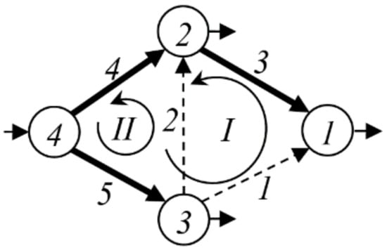
Figure 3. A scheme. Thick lines are spanning tree branches, and dashed arrows are chords.

As seen, the matrices $A_T^T$, ${\mathsf{\Phi }}_T,{\mathsf{\Phi }}_T^{-1}$ are upper triangular. ${({\mathsf{\Phi }}_T^{-1})}_{ij}\ne 0$, if there is a directed path from node $j$ to node $i$, and ${({\mathsf{\Phi }}_T^{-1})}_{ij}=0$, otherwise. The structure of matrix ${\mathsf{\Phi }}_C{\mathsf{\Phi }}_T^{-1}$ is identical to $B_T$. Matrices $\tilde{M}$ and $K$ are diagonally dominant (by absolute value), and symmetrical in structure but not in values of their elements.

7. Numerical Case Study

Let us consider a numerical case study on the application of proposed methods to a fragment of the high-pressure gas transmission system [21], presented in Figure 4.

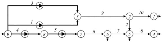
Figure 4. Scheme of a gas transmission system. Thick lines correspond to a compressor, thin lines—to pipeline sections.

All pipeline sections are horizontal and modeled by the relationship $\left|p_{\mathrm{H},i}\right|p_{\mathrm{H},i}-\left|p_{\mathrm{K},i}\right|p_{\mathrm{K},i}=s_i{x}_i\left|x_i\right|$, $i=2,\overline{6,10}$, with $s_2$ = 0.006; $s_6$ = 0.253; $s_7$ = 4.757; $s_8$ = 0.436; $s_9$ = 1.332; $s_{10}$ = 0.349. Relationships for compressor have the form

$$\phi (p_{\mathrm{H},i},p_{\mathrm{K},i},x_i)=\left({\beta }_{0,i}+\frac{{\beta }_{1,i}^2}{4{\beta }_{2,i}}\right)p_{\mathrm{H},i}\left|p_{\mathrm{H},i}\right|-p_{\mathrm{K},i}\left|p_{\mathrm{K},i}\right|-{\beta }_{2,i}\left(x_i-\frac{{\beta }_{1,i}}{2{\beta }_{2,i}}{p}_{\mathrm{H},i}\right)\left|x_i-\frac{{\beta }_{1,i}}{2{\beta }_{2,i}}{p}_{\mathrm{H},i}\right|=0$$

and values of their coefficients are indicated in Table 1.

Table 1. Coefficients of compressor characteristics.

i	${\mathit{\beta }}_{0,\mathit{i}}$	${\mathit{\beta }}_{1,\mathit{i}}$	${\mathit{\beta }}_{2,\mathit{i}}$
1	1.040975262	0.4520492230	0.1660378943
3	1.040975262	0.4520492230	0.1660378943
4	1.056105913	0.4352722015	0.2396158372
5	1.049124727	0.3668417249	0.1867004063

Derivatives of this relationship have the form ${\left(\frac{\partial \phi }{\partial x}\right)}_i=-2{\beta }_{2,i}\left|x-\frac{{\beta }_{1,i}{p}_{\mathrm{H},i}}{2{\beta }_{2,i}}\right|$, ${\left(\frac{\partial \phi }{\partial p_{\mathrm{H}}}\right)}_i=2\left|p_{\mathrm{H},i}\right|\left({\beta }_{0,i}+\frac{{\beta }_{1,i}^2}{4{\beta }_{2,i}}\right)-{\beta }_{1,i}{x}_i-\frac{{\beta }_{1,i}{p}_{\mathrm{H},i}}{2{\beta }_{2,i}}\cdot sign\left(x_i-\frac{{\beta }_{1,i}{p}_{\mathrm{H},i}}{2{\beta }_{2,i}}\right)$, ${\left(\frac{\partial \phi }{\partial p_{\mathrm{K}}}\right)}_i=-2\left|p_{\mathrm{K},i}\right|$.

Withdrawals at nodes (million m³/day) are $Q_1$ = 19.1; $Q_4$ = 14.8; $Q_5$ = 0.632; $Q_6$ = 0.32. Set pressure is $P_9$ = 33.778 at.

The following technique is used to obtain the initial approximation $P^0$ in the MNM, which is equivalent to the initial approximation $x^0$ employed in MLM. Let an arbitrary value $x_C^0$ be set, then $x_T^0=A_T^{-1}(Q-A_C{x}_C^0)$, and $P^0$ is determined from ${\phi }_T(P^0,x_T^0)=0$.

The results of calculating the MLM by iterations are shown in Table 2, Table 3 and Table 4. In this study, $x_C^0=\{x_1^0,x_2^0\}$. As seen, the initial approximation (k = 0) is rather far from the solution. It has the flow values opposite to the orientations of branches, and negative pressure values that are beyond the solution. Nevertheless, both methods provide monotonic convergence, which is illustrated in Figure 5. Here, for MNM $‖u_1‖=\log \left(\underset{1\le j\le m-1}{\max }\left|u_{1,j}\right|\right)$, and for MLM $‖u_2‖=\log \left(\underset{1\le r\le c}{\max }\left|{\phi }_{C,r}^k\right|\right)$. Thus, the MNM required 6 iterations (with step length regulation), while MLM needed only 4 iterations.

Table 2. Flow rates and pressures for iterations.

i\k	0	1	2	3	4	j\k	0	1	2	3	4
1	10.00	14.45	10.70	10.80	10.80	1	−24.03	30.49	31.60	31.55	31.55
2	20.00	4.04	2.44	2.50	2.50	2	−21.22	32.51	33.56	33.51	33.51
3	29.10	8.68	10.84	10.80	10.80	3	39.83	42.07	41.76	41.76	41.76
4	−4.24	11.72	13.32	13.25	13.25	4	50.05	35.33	31.91	32.05	32.05
5	−4.24	11.72	13.32	13.25	13.25	5	50.99	36.65	33.37	33.51	33.51
6	−4.24	11.72	13.32	13.25	13.25	6	50.01	44.29	43.78	43.80	43.80
7	−4.56	11.40	13.00	12.93	12.93	7	49.96	44.68	44.29	44.31	44.31
8	14.80	14.80	14.80	14.80	14.80	8	41.51	38.94	38.77	38.77	38.77
9	39.10	23.14	21.54	21.60	21.60	9	33.78	33.78	33.78	33.78	33.78
10	19.10	19.10	19.10	19.10	19.10

Table 3. Derivative values over iterations.

i\k	1			2			3			4
	${\chi }_i$	${\eta }_i$	${\kappa }_i$	${\chi }_i$	${\eta }_i$	${\kappa }_i$	${\chi }_i$	${\eta }_i$	${\kappa }_i$	${\chi }_i$	${\eta }_i$	${\kappa }_i$
1	−11.95	74.84	−79.65	−10.47	76.86	−84.14	−11.72	75.16	−83.52	−11.68	75.21	−83.53
2	−0.24	42.44	−101.98	−0.05	65.02	−73.31	−0.03	67.11	−66.74	−0.03	67.02	−67.02
3	−5.61	83.48	−79.65	−12.39	74.25	−84.14	−11.67	75.22	−83.52	−11.68	75.21	−83.53
4	−16.74	69.50	−83.01	−9.09	76.45	−77.89	−8.32	77.14	−77.53	−8.35	77.12	−77.54
5	−16.81	85.53	−99.93	−9.91	86.01	−89.35	−9.25	86.22	−88.59	−9.27	86.22	−88.62
6	−2.15	99.93	−100.02	−5.93	89.35	−88.57	−6.74	88.59	−87.57	−6.71	88.62	−87.61
7	−43.46	100.02	−101.98	−108.42	88.57	−73.31	−123.64	87.57	−66.74	−123.05	87.61	−67.02
8	−12.94	101.98	−100.09	−12.91	73.31	−70.66	−12.91	66.74	−63.82	−12.91	67.02	−64.11
9	−104.16	79.65	−42.44	−61.63	84.14	−65.02	−57.37	83.52	−67.11	−57.54	83.53	−67.02
10	−13.33	42.44	−48.07	−13.33	65.02	−60.97	−13.33	67.11	−63.21	−13.33	67.02	−63.11

Table 4. The values of the coefficients of the system of equations, the right-hand side and the results of its solution by iterations.

k	${\mathit{K}}^{\mathit{k}}$	${\mathit{\phi }}_{\mathit{C}}^{\mathit{k}}$	$\mathsf{\Delta }{\mathit{x}}_{\mathit{C}}^{\mathit{k}}$
1	$\left[\begin{array}{cc}-17.55& 5.61\\ 5.61& -189.68\end{array}\right]$	$\left[\begin{array}{r}\hfill -167.65\\ \hfill 3052.93\end{array}\right]$	$\left[\begin{array}{r}\hfill 4.45\\ \hfill -15.96\end{array}\right]$
2	$\left[\begin{array}{rr}\hfill -22.86& \hfill 12.39\\ \hfill 12.39& \hfill -208.36\end{array}\right]$	$\left[\begin{array}{r}\hfill 65.92\\ \hfill 286.90\end{array}\right]$	$\left[\begin{array}{r}\hfill -3.75\\ \hfill -1.60\end{array}\right]$
3	$\left[\begin{array}{rr}\hfill -22.39& \hfill 11.67\\ \hfill 11.67& \hfill -217.96\end{array}\right]$	$\left[\begin{array}{r}\hfill -1.57\\ \hfill -12.39\end{array}\right]$	$\left[\begin{array}{r}\hfill 0.10\\ \hfill 0.06\end{array}\right]$
4	$\left[\begin{array}{rr}\hfill -23.37& \hfill 11.68\\ \hfill 11.68& \hfill -217.57\end{array}\right]$	$\left[\begin{array}{r}\hfill 0\\ \hfill 0.11\end{array}\right]$	$\left[\begin{array}{r}\hfill 0\\ \hfill 0\end{array}\right]$

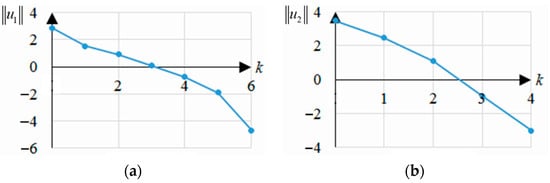
Figure 5. Process of convergence: (a) modified node method (MNM); (b) modified loop method (MLM).

Figure 6 shows the results of testing MNM and MLM on 100 vectors of initial approximations, which were generated by a generator of random uniformly distributed numbers: for MNM $-100\le P_j^0\le 100,j=\overline{1,m-1}$; for MLM $-100\le x_i^0\le 100,i=\overline{1,c}$. Iteration stopping criteria are for MNM $\underset{1\le j\le m-1}{\max }\left|\mathsf{\Delta }{P}_j^k\right|<0.01$, $\underset{1\le j\le m-1}{\max }\left|{(u_1^k)}_j\right|<0.01$; for MLM $\underset{1\le r\le c}{\max }\left|{\phi }_{C,r}^k\right|<0.01$.

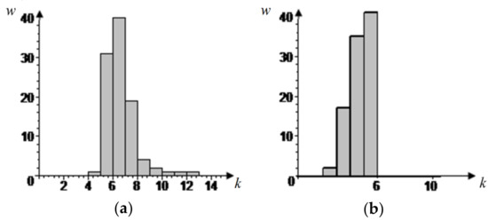
Figure 6. The number of calculated conditions w (%) under which the problem is solved in k iterations for: (a) MNM; (b) MLM.

The study indicates that: (1) both methods demonstrate strong convergence; (2) the number of iterations weakly depends on the proximity of the initial approximation to the solution; (3) MLM requires on average fewer iterations than MNM. Note also that the number of iterations weakly depends on the scheme dimension; however, as indicated, the computational costs for each iteration depend on the topology of a particular scheme.

8. Conclusions

Analysis of the available variety of methods for calculating isothermal steady-state flow distribution in pipeline systems designed for various purposes shows their significant dependence on the specifics of models of the medium flow for individual elements. The analysis has also demonstrated the absence of methods that are equally applicable in the general case. The main types of such models are highlighted, including traditional, implicit by flow rate, and pressure-dependent ones. The research shows general conditions for their application to ensure the existence and uniqueness of a solution to the flow distribution problem.

Against the background of a brief description of the generalized MNM put forward in our previous studies, we propose a new loop method. Both methods are universal with regard to the specificity of flow models, coincide with conventional methods in the particular case of classical flow models, but each of them has its area of preferred application depending on the PLS topology.

We propose the methods for algorithmizing the generalized loop method, which provide the computational costs lower than those of the well-known technique of double iteration cycles and comparable to those of the classical MLM.

References

- Merenkov, A.P.; Khasilev, V.Y. Theory of Hydraulic Circuits; Nauka: Moscow, Russia, 1985. [Google Scholar]
- Merenkov, A.; Novitsky, N.; Sidler, V. Direct and inverse problems of flow distribution in hydraulic. Soviet. Techno. Rev. Sec. Energy Rev. 1994, 7, 33–95. [Google Scholar]
- Berge, C. Théorie des Graphes et ses Applications; Dunod: Paris, France, 1958; p. 275. [Google Scholar]
- Todini, E.; Rossman, L.A. Unified framework for deriving simultaneous equation algorithms for water distribution networks. J. Hydraul. Eng. 2013, 139, 511–526. [Google Scholar] [CrossRef]
- Andriashev, M.M. Technique of Water Supply Networks Analysis; Sov. zakonodatelstvo: Moscow, Russia, 1932. [Google Scholar]
- Lobachev, V.G. A new method for water supply ring mains linking in the analysis of water supply networks. Sanit. Tekhnika 1934, 2, 8–12. [Google Scholar]
- Cross, H. Analysis of Flow in Networks of Conduits or Conductors; University of Illinois at Urbana Champaign, College of Engineering Experiment Station: College Station, TX, USA, 1936; Available online: http://hdl.handle.net/2142/4433 (accessed on 1 January 2021).
- Brkic, D. An improvement of Hardy Cross method applied on looped spatial natural gas distribution networks. Appl. Energy 2009, 86, 1290–1300. [Google Scholar] [CrossRef]
- Merenkov, A.P.; Sennova, E.V.; Sumarokov, S.V.; Sidler, V.G. Mathematical Modeling and Optimization of Heat, Water, Oil, and Gas Supply Systems; VO “Nauka”, Siberian Publishing Company: Novosibirsk, Russia, 1992. [Google Scholar]
- Novitsky, N.N.; Alekseev, A.V.; Grebneva, O.A.; Lutsenko, A.V.; Tokarev, V.V.; Shalaginova, Z.I. Multilevel modeling and optimization of large-scale pipeline systems operation. Energy 2019, 184, 151–164. [Google Scholar] [CrossRef]
- Brkic, D. Iterative Methods for Looped Network Pipeline calculation. Water Resour. Manag. 2011, 25, 2951–2987. [Google Scholar] [CrossRef]
- Woldeyohannes, A.D.; Majid, M.A.A. Simulation model for natural gas transmission pipeline network system. Simul. Model. Pract. Theory 2011, 19, 196–212. [Google Scholar] [CrossRef]
- Osiadacz, A.J.; Pienkosz, K. Methods of steady-state simulation for gas networks. Int. J. Syst. Sci. 1988, 19, 1311–1321. [Google Scholar] [CrossRef]
- Mikhailovsky, E.M.; Novitsky, N.N. A modified nodal pressure method for calculating flow distribution in hydraulic circuits for the case of unconventional closing relations. St. Petersburg Polytech. Univ. J. Phys. Math. 2015, 1, 120–128. [Google Scholar] [CrossRef]
- Houghtalen, R.; Akan Osman, A.H.; Hwang, N. Fundamentals of Hydraulic Engineering Systems, 5th ed. Published by Pearson. 2017. Available online: https://www.pearson.com/uk/educators/higher-education-educators/program/Houghtalen-Fundamentals-of-Hydraulic-Engineering-Systems-5th-Edition/PGM1091329.html (accessed on 1 April 2021).
- Colebrook, C.F. Turbulent flow in pipes, with particular reference to the transition region between smooth and rough pipe laws. Jour. Ist. Civil Engrs. 1939, 11, 133–156. [Google Scholar] [CrossRef]
- Olivares, A.; Guerra, R.; Alfaro, M.; Notte-cuello, E.; Puentes, L. Experimental evaluation of correlations used to calculate friction factor for turbulent flow in cylindrical pipes. Rev. Int. De Métodos Numéricos Para Cálculo Y Diseño En Ing. 2019, 35. [Google Scholar] [CrossRef]
- Stepanoff, A.J. Turboblowers: Theory, Design and Application of Centrifugal and Axial Flow Compressors and Fans; John Willey & Sons, Inc.; Chapman & Hall, Ltd.: New York, NY, USA, 1958. [Google Scholar]
- Campsty, N.A. Compressors Aerodynamics; Longman Scientific & Technical: Harlow, UK, 1989; Available online: http://www.pearsonlongman.com/ (accessed on 1 April 2021).
- Nemudrov, A.G.; Chernikin, V.I. Analysis of gas pipeline operation modes based on the method of determining the optimal characteristics of turbochargers. Gazov. Promyshlennost 1966, 3, 31–34. [Google Scholar]
- Evdokimov, A.G.; Tevyashev, A.D. Operational Control of Flow Distribution in Utilities; Vishcha Shkola; Kharkiv University Publishing House: Kharkiv, Ukraine, 1980; Available online: https://www.univer.kharkov.ua/ru/general/structure/publish (accessed on 1 April 2021).
- Ekhtiari, A.; Dassios, I.; Liu, M.; Syron, E. A novel approach to model a gas network. Appl. Sci. 2019, 9, 1047. [Google Scholar] [CrossRef]
- Cavalieri, F. Steady-state flow computation in gas distribution networks with multiple pressure levels. Energy 2017. [Google Scholar] [CrossRef]
- Kirillov, P.L.; Yuryev, Y.S.; Bobkov, V.P. Handbook on Thermo-Hydraulic Analysis; Kirillov, P.L., Ed.; Energoatomizdat: Moscow, Russia, 1990. [Google Scholar]
- Levin, A.A.; Tairov, E.A.; Chistyakov, V.F. Application of the hydraulic circuit theory to modeling of heat and power units. Izv. Ran Energy 2011, 2, 142–147. [Google Scholar]
- Ivanov, V.A. Steady-State and Transient Modes of High-Capacity Steam Turbine Plants; Energiya: Leningrad, Russia, 1971. [Google Scholar]
- Korelshtein, L.B.; Pashenkova, E.S. Experience of using global gradient methods in the analysis of the steady isothermal flow of liquids and gases in pipelines. In Pipeline Systems of the Energy Industry: Developments of the Theory and Methods of Mathematical Modeling and Optimization; Averyanov, V.K., Novitsky, N.N., Sukharev, M.G., Eds.; Nauka: Novosibirsk, Russia, 2008; pp. 80–89. [Google Scholar]
- Pankratov, V.S.; Dubinsky, A.V.; Sipershtein, B.I. Information and Computer Systems in Supervisory Control of Gas Pipelines; Nedra: Leningrad, Russia, 1988. [Google Scholar]
- Bermudez, A.; Shabani, M. Modelling compressors, resistors and valves in finite element simulation of gas transmission networks. Appl. Math. Model. 2021, 89, 1316–1340. [Google Scholar] [CrossRef]
- Brkic, D.; Praks, P. An efficient iterative method for looped pipe network hydraulics free of flow-corrections. Fluids 2019, 4, 73. [Google Scholar] [CrossRef]
- Chionov, A.M.; Kazak, K.A.; Kulik, V.S. Modeling of the pipeline system in the stationary mode. Zhurnal Neftegazov. Stroit. 2014, 2, 54–59. [Google Scholar]
- Merenkov, A.P. Differenciacija metodov rascheta gidravlicheskih cepej. Zhurn. Vychisl. Mat. I Fiz. 1973, 13, 1237–1248. [Google Scholar]
- Todini, E.; Pilati, S. A gradient algorithm for the analysis of pipe networks. Comput. Appl. Water Supply 1988, 1, 1–20. [Google Scholar]
Publisher’s Note: MDPI stays neutral with regard to jurisdictional claims in published maps and institutional affiliations. |
© 2021 by the authors. Licensee MDPI, Basel, Switzerland. This article is an open access article distributed under the terms and conditions of the Creative Commons Attribution (CC BY) license (https://creativecommons.org/licenses/by/4.0/).