Counting Hamiltonian Cycles in 2-Tiled Graphs

Abstract

In 1930, Kuratowski showed that $K_{3,3}$ and $K_5$ are the only two minor-minimal nonplanar graphs. Robertson and Seymour extended finiteness of the set of forbidden minors for any surface. Širáň and Kochol showed that there are infinitely many k-crossing-critical graphs for any $k\ge 2$, even if restricted to simple 3-connected graphs. Recently, 2-crossing-critical graphs have been completely characterized by Bokal, Oporowski, Richter, and Salazar. We present a simplified description of large 2-crossing-critical graphs and use this simplification to count Hamiltonian cycles in such graphs. We generalize this approach to an algorithm counting Hamiltonian cycles in all 2-tiled graphs, thus extending the results of Bodroža-Pantić, Kwong, Doroslovački, and Pantić.

1. Introduction

In 1930, Kuratowski characterized graphs that can be drawn in a plane with no crossings [1]. His research was an opening step for several directions characterizing graph families using forbidden substructures, such as extremal graph theory that forbids any subgraph isomorphic from being in a given graph [2], and the related structural graph theory emanating from forbidding induced subgraphs, for instance, several characterizations of Trotter and Moore [3] as well as perfect graph theorems [4,5]. Robertson, Seymour, and others extended these results to graph minor theory [6,7]. While far from complete, a more detailed review of the related research emanating from Kuratowski theorem is presented in the next section. In this introduction, we only focus on the two topics that are fundamental to the results of our paper, crossing-critical graphs and graph Hamiltonicity.

Observe (as is elaborated in the next section), that Kuratowski graphs can be interpreted as the only two 3-connected 1-crossing-critical graphs. A parallel theorem describing all 2-crossing-critical graphs was established by Bokal, Oporowski, Salazar, and Richter [8], who characterized the complete list of minimal forbidden subdivisions for a graph to be realizable in a plane with only one crossing. They exhibit a significantly richer structure: unlike just two 3-connected 1-crossing-critical graphs, the graphs realizable in a plane with at most one crossing already exhibit infinite families of topologically minimal obstruction graphs. Although it cannot be claimed that all these 2-crossing-critical graphs are Hamiltonian (with Petersen graph being the most known counterexample), the claim is fairly easy to see for large such graphs using the aforementioned characterization of 2-crossing-critical graphs. Hence, almost all of these graphs are Hamiltonian. In this paper, we address a significantly more difficult problem of counting their different Hamiltonian cycles. The interest in understanding the number of different Hamiltonian cycles in various graph families originates from biochemical modelling of the polymers [9], where a collapsed polymer globule is modelled by a Hamiltonian cycle and the number of Hamiltonian cycles corresponds to the entropy of a polymer system in a collapsed but disordered phase. This shows an interesting intuitive duality to counting Eulerian cycles that showed relevance in constructing controlled, de novo protein structure folding [10,11]. In 1990, a characterization of Hamiltonian cycles of the Cartesian product $P_4\square P_n$ was established [12]. In 1994, Kwong and Rogers developed a matrix method for counting Hamiltonian cycles in $P_m\square P_n$, obtaining exact results for $m=4,5$ [13]. Their method was extended to arbitrarily large grids by Bodroža-Pantić et al. [14] and by Stoyan and Strehl [15]. Later, Bodroža-Pantić et al. gave some explicit generating functions for the number of Hamiltonian cycles in graphs $P_m\square P_n$ and $C_m\square P_n$ [16,17]. Earlier, Saburo developed a field theoretic approximation of the number of Hamiltonian cycles in graphs $C_m\square C_n$ in [18] as well as in planar random lattices [19]. Fireze et al. considered generating and counting Hamiltonian cycles in random regular graphs [20]. Given these results, we note that our approach renders large 2-crossing-critical graphs to be the first nonplanar graph family for which the number of Hamiltonian cycles can be exactly determined. It may be relevant that the dissertation [21] similarly investigates links between 2-crossing-critical graphs, graph embeddings, and Hamiltonian cycles in higher surfaces.

In addition to an alphabetic description of large 2-crossing-critical graphs that allows for specifying the above formulae and may inspire further investigation of this graph class and ease access to graph-theoretic research building in this next step beyond the Kuratowski theorem, we hence extend this body of research on counting Hamiltonian cycles by going beyond Cartesian products of paths and cycles and apply the matrix method for counting Hamiltonian cycles to general 2-tiled graphs, which by the previously mentioned characterization theorem includes almost all 2-crossing-critical graphs. By allowing for nonplanar graphs in our approach, a new type of Hamiltonian cycle not observed previously appears. We complement the previous approaches of devising generating functions (which is feasible for well-structured graphs, such as aforementioned Cartesian products, or for the expected number of Hamiltonian cycles in random graphs) by an algorithm, which is in the case of 2-crossing-critical graphs implementable in linear time. For certain subfamilies of 2-crossing-critical graphs, the algorithm can even be simplified to a closed formula, using only the counts of specific letters in our alphabetic representation of the 2-crossing-critical graph, thus rendering these graphs the first nonplanar graphs for which an exact number of distinct Hamiltonian cycles is known. Specifically, we constructively prove the following theorems:

Theorem 1.

Let G be a 2-connected 2-crossing-critical graph containing a subdivision $H\simeq V_{10}$. There exists an algorithm of linear time complexity in the number of vertices of G that computes the number of Hamiltonian cycles in G.

The theorem has the following easier-to-state corollary:

Corollary 1.

There exists an integer N such that any 2-connected 2-crossing-critical graph G with at least N vertices is Hamiltonian.

As Petersen graph is a 3-connected 2-crossing-critical graph and is not Hamiltonian, containing a $V_{10}$ subdivision (or, equivalently, being large) cannot simply be ommited for the above conclusions. For a picture of $V_{10}$, see Figure 1.

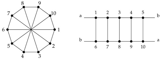
Figure 1. Two pictures of $V_{10}$. In general, $V_{2n}$ is obtained from a $2n$-cycle by adding the n main diagonals.

The algorithm in Theorem 1 is a special case of the general algorithm from the following theorem:

Theorem 2.

Let $\mathcal{T}$ be a finite family of 2-tiles, and let $\mathcal{G}$ be a family of cyclizations of finite sequences of such tiles. There exists an algorithm that yields, for each graph $G\in \mathcal{G}$, the number of distinct Hamiltonian cycles in G. For a fixed set $\mathcal{T}$, the run time of the algorithm is quadratic in the number of tiles (and hence vertices) of G.

The rest of the paper is organized as follows. In the next section, we put the central concept of tiled graphs and crossing-critical graphs into the wider context of graph theory research. We introduce tiles and tiled graphs in Section 3, where a general algorithm for counting Hamiltonian cycles in 2-tiled graphs is presented. In Section 4, we introduce 2-crossing-critical graphs and the recent characterization of large such graphs as 2-tiled graphs. In Section 5, we combine the results by adapting the general counting algorithm to 2-crossing-critical graphs and constructively prove the above key results.

2. Related Research

Kuratowski theorem inspired several characterizations of graph families using forbidden subgraphs, which paved paths to significantly different areas of graph theory. Extremal graph theory is concerned with forbidding any subgraph isomorphic from being in a given graph [2] and maximizing the number of edges under this constraint. Significant structural theory was developed when forbidden subgraphs were replaced by forbidden induced subgraphs, for instance, several characterizations of Trotter and Moore [3] and the remarkable weak and strong perfect graph theorems [4,5].

Interest has also been shown in finding forbidden subgraphs that imply Hamiltonicity of graphs. In 1974, Goodman and Hedetniemi showed that a graph not containing induced $K_{1,3}$ and $K_{1,3}+e$, where e creates a 3-cycle, is Hamiltonian [22]. A series of several similar results was closed in 1997 by Faudree and Gould, who characterized all pairs of graphs such that forbidding their induced presence in a graph implies a graph’s Hamiltonicity [23]. This was via several papers extended to a complete characterization of triples of forbidden graphs implying Hamiltonicity, the final one being [24].

Graph minor theory extended the Kuratowski theorem to higher surfaces, showing that the set of graphs embeddable into any surface can be characterized by a finite set of forbidden minors [7]. The exact characterization was devised by Archdeacon for the projective plane [6], but already on the torus, the number of forbidden minors reached tens of thousands [25]. Mohar devised algorithms to embed graphs on surfaces [26], which was later improved by Kawarabayashi, Mohar, and Reed [27]. Characterizations of graph classes with subdivisions received somewhat less renowned attention. Early on the above path, Chartrand, Geller, and Hedetniemi pointed at some common generalizations of forbidding a small complete graph and a corresponding complete bipartite subgraph as a subdivision, resulting in empty graphs, trees, outerplanar graphs, and planar graphs [28]. That unifying approach apparently did not yield fruitful results, but more recently, Dvořák established a characterization of several graph classes using forbidden subdivisions [29], thus reaching even outside of topological graph theory.

The cornerstone of our contribution is yet another generalization of Kuratowski theorem. Note that the theorem elementarily implies that the two Kuratowski graphs $K_5$ and $K_{3,3}$ are the only 3-connected graphs that need at least one crossing to be drawn in a plane, but each their proper subgraph is planar and hence has a strictly smaller crossing number. Furthermore, all the graphs with the latter property can be obtained from them by subdividing their edges. Using the definition from the next section, Kuratowski theorem characterizes all 3-connected 1-crossing-critical graphs and consequently describes all 1-crossing critical graphs as their subdivisions.

It was already known that, contrary to fixed-genus-embeddable graphs, fixed-crossing-number realizable graphs exhibit a richer structure of topologically minimal obstruction graphs, as first demonstrated by Šiřan [30] constructing infinite families of c-crossing-critical graphs. Kochol extended this result to simple, 3-connected graphs [31].

A parallel to this interpretation of Kuratowski theorem but for 2-crossing-critical graphs was established recently by Bokal, Oporowski, Salazar, and Richter [8]. They characterized the complete list of minimal forbidden subdivisions for a graph to be realizable in a plane with only one crossing, i.e., 2-crossing-critical graphs. They showed that all such graphs are either small or 2-connected and obtained from 3-connected ones using subdivisions and similar operations, or 3-connected and obtained similarly as Kochol 2-crossing-critical graphs [31] but using 42 different structures (of which Kochol used just one). Later in this paper, we formalize these structures as tiles.

Tiles as a central tool in graph theory were first formally defined by Pinontoan and Richter [32], who extended the answer to Salazar’s question on average degrees in infinite families of c-crossing-critical graphs [33]. Salazar’s question was resolved by Bokal, again using tiles. They were instrumental in further studies on degrees in crossing critical graphs by Hliněný [34], whose most complete results so far are published in [35]. Most of this desire for understanding the degrees in crossing-critical graphs was inspired by a conjecture of Richter that c-crossing-critical graphs have their maximum degree bounded from above by a function of c. The conjecture was first existentially disproved by Dvořák and Mohar [36]. A constructive counterexample was obtained by Bokal et al. [37], who also showed that bounded degree conjecture holds precisely for $c\le 12$. Instrumental in this result were wedges, a degenerate form of tiles that has yet to be formalized. Tiles, wedges, and planar belts were shown to be (in addition to a small connecting graph) the three key ingredients of large c-crossing-critical graphs by Dvořák, Hliněný, and Mohar [38].

In addition to applications of tiles for studying crossing-critical graphs, Pinontoan and Richter opened another direction of results. They studied the limit crossing number of tiled graphs, showing the existence of a limit crossing number for a periodic family of graphs (in the terms defined later, k-tiled graphs resulting from the cyclizations of repeated joins of a single tile). Richter later asked whether this limit is computable, which was proven by Dvořák and Mohar in [39]. Some further graph invariants on 2-crossing-critical graphs were obtained in parallel with our results and published in [40].

It may be interesting to note that tiles and their joins are a specific kind of labeled graphs and operations on them, as introduced in Lovász’es seminal book on large networks and graph limits [41]. Hence, introductory understanding of the conceptspresented here may motivate researchers in pursuit of that direction. We do not harmonize the notation here, but it may be feasible to do so when extending the theory of tiles to the theory of earlier mentioned wedges.

3. Hamiltonian Cycles in 2-Tiled Graphs

In this section, we introduce the concept of a tile that was introduced in [32] and later redesigned in [42] and applied in [8,35] and the k-tiled graphs. We use the notation from [8]. To facilitate brevity, we have prepared Table A1 with a summary of frequently used notation. It is located in the appendix.

Definition 1.

A tile is a triple $T=(G,x,y)$, consisting of a connected graph G and two sequences $x=(x_1,x_2,\dots ,x_k)$ (left wall) and $y=(y_1,y_2,\dots ,y_l)$ (right wall) of distinct vertices of G, with no vertex of G appearing in both x and y. If $\left|x\right|=\left|y\right|=k$, we call T a k-tile.

We use the following notation when combining tiles:

Definition 2.

1.

The tiles $T=(G,x,y)$ and $T^{\prime }=(G^{\prime },x^{\prime },y^{\prime })$ are compatible whenever $\left|y\right|=|x^{\prime }|.$

2.

A sequence $\mathcal{T}=(T_0,T_1,\dots ,T_m)$ of tiles is compatible if, for each $i\in \{1,2,\dots ,m\}$, $T_{i-1}$ is compatible with $T_i$.

3.

The join of compatible tiles $(G,x,y)$ and $(G^{\prime },x^{\prime },y^{\prime })$ is the tile $T=(G,x,y)\otimes (G^{\prime },x^{\prime },y^{\prime })$ for which the graph is obtained from disjoint union of G and $G^{\prime }$ by identifying the sequence y term by term with the sequence $x^{\prime }$.

4.

The join of a compatible sequence $\mathcal{T}=(T_0,T_1,\dots ,T_m)$ of tiles is defined as $\otimes \mathcal{T}=T_0\otimes T_1\otimes \cdots \otimes T_m$.

5.

A tile T is cyclically compatible if T is compatible with itself.

6.

For a cyclically compatible tile $T=(G,x,y)$, the cyclization of T is the graph $\circ T$ obtained by identifying the respective vertices of x with y.

7.

A cyclization of a cyclically compatible sequence of tiles $\mathcal{T}$ is defined as $\circ \mathcal{T}=\circ (\otimes \mathcal{T})$.

8.

A k-tiled graph is a cyclization of a sequence of at least $(k+1)$k-tiles.

Lemma 1.

Let C be a Hamiltonian cycle in a 2-tiled graph $G=\circ (T_0,T_1,\dots ,T_m)$. Then, we have the following:

1.

$C=\bigcup _{i=0}^m(C\cap T_i)$.

2.

$C\cap T_i$ is a union of paths and isolated vertices.

3.

Let v be a vertex of a component of $C\cap T_i$. Then, v has degree 2 in $C\cap T_i$ or v is a wall vertex.

4.

There are at most two distinct non-degenerate paths in $C\cap T_i$.

5.

If $C\cap T_i$ consists of distinct non-degenerate paths $P_1$ and $P_2$, then $C\cap T_i=P_1\oplus P_2$.

Proof. 

• $C=C\cap G=C\cap \left(\bigcup _{i=0}^m{T}_i\right)\stackrel{\mathrm{Distributive}\mathrm{law}}{=}\bigcup _{i=0}^m(C\cap T_i).$
• Let K be a component of $C\cap T_i$. As C is a cycle, K is a connected subgraph of C. Then, K is either equal to C, a path, or a vertex. If $K=C$, then $T_i$ contains all the vertices of G, a contradiction to $m\ge 2$ (in at least one tile, C does not contain all the vertices). The claim follows.
• Let v be a vertex of $C\cap T_i$ of degree different from 2. As maximum degree in C is 2, v has degree 1 or 0. If v is an internal vertex of $T_i$, its degree in $C=\bigcup _{i=0}^m(C\cap T_i)$ is equal to its degree in $C\cap T_i$. This contradicts C being a cycle and the claim follows.
• By Claim 3, paths start and end in a wall vertex. Each distinct non-degenerate path needs two unique wall vertices, and the claim follows.
• By Claim 4, $P_1$ and $P_2$ contain all the wall vertices. By Claim 3, isolated vertices can only be wall vertices; hence, there are no isolated vertices and $C\cap T_i=P_1\oplus P_2$.

□

Corollary 2.

Let C be a Hamiltonian cycle in a 2-tiled graph $G=\circ (T_0,T_1,\dots ,T_m)$ and $N_i$ be the set of all isolated vertices in $C\cap T_i$. Then, $(C\cap T_i)\setminus N_i$ is one of the following:

1.

A path that begins in a vertex of the left wall, ends in a vertex of the right wall, and covers all internal vertices of $T_i$.

2.

A pair of distinct paths for which each begins and ends at opposite walls, span $T_i$, and respect the vertex order of the walls.

3.

A pair of distinct paths for which each begins and ends at opposite walls, span $T_i$, and invert the vertex order of the walls.

4.

An empty set.

5.

A pair of distinct paths for which each begins and ends at the same wall and span $T_i$.

6.

A path that begins and ends at the same wall and covers all internal vertices of $T_i$.

We say that a path “traverses” a 2-tile, if it starts at the left wall and ends at the right wall of a 2-tile. Based on Corollary 2, we define three groups of C-types of tiles as follows:

Definition 3.

Let C be a Hamiltonian cycle in a 2-tiled graph $G=\circ (T_0,T_1,\dots ,T_m)$, $x=(x_1,x_2)$ be the left, and $y=(y_1,y_2)$ be the right wall of $T_i$.

1.

If a cycle C traverses $T_i$ with a single path and covers all internal vertices of $T_i$, then we say that $T_i$ is of zigzagging C-type, of which there exist four kinds, relevant for completing the Hamiltonian cycles between the tiles.

First, $T_i$ is of zigzagging C-type ${}_{\left\{x_{3-j}\right\}}{-}_{\left\{y_{3-k}\right\}}$ if $C\cap T_i$ contains a single path P, the endvertices of P are vertices $x_j$ and $y_k$ of distinct walls of $T_i$, and P contains the non-endvertex wall vertices $x_{3-j},y_{3-k}$. If either wall vertex that is not an endvertex of P is not contained in P, then $C\cap T_i$ contains a path P and these vertices as isolated vertex components. We denote such isolated components using an overline, leading to zigzagging C-types ${}_{\left\{x_{3-j}\right\}}{-}_{\left\{{\overline{y}}_{3-k}\right\}},{}_{\left\{{\overline{x}}_{3-j}\right\}}{-}_{\left\{y_{3-k}\right\}},{}_{\left\{{\overline{x}}_{3-j}\right\}}{-}_{\left\{{\overline{y}}_{3-k}\right\}}$.

2.

If a cycle C traverses $T_i$ with a pair of distinct traversing paths that span $T_i$, then we say that $T_i$ is of traversing C-type.

(a)

$T_i$ is of aligned (Aligned pairs of traversing paths were introduced in [8].) traversing C-type = if $C\cap T_i$ contains a pair of distinct paths $P_1$ and $P_2$, the endvertices of $P_1$ are $x_1$ and $y_1$, and the endvertices of $P_2$ are $x_2$ and $y_2$.

(b)

$T_i$ is of twisted (Twisted pairs of traversing paths were introduced in [8].) traversing C-type × if $C\cap T_i$ contains a pair of distinct paths $P_1$ and $P_2$, the endvertices of $P_1$ are $x_1$ and $y_2$, and the endvertices of $P_2$ are $x_2$ and $y_1$.

3.

If a cycle C does not traverse $T_i$, then we say that $T_i$ is of flanking C-type.

(a)

$T_i$ is of flanking C-type ∅ if $C\cap T_i$ is an empty graph spanned by $\{x_1,x_2,y_1,y_2\}$.

(b)

$T_i$ is of flanking C-type ‖ if $C\cap T_i$ contains a pair of distinct paths $P_1$ and $P_2$, the endvertices of $P_1$ are $x_1$ and $x_2$, and the endvertices of $P_2$ are $y_1$ and $y_2$.

(c)

$T_i$ is of flanking C-type ${|}_{\{y_1,y_2\}}$ if $C\cap T_i$ contains a single path P, the endvertices of P are $x_1,x_2$ of the same wall of $T_i$, and P contains the non-endvertex wall vertices $y_1,y_2$. If either wall vertex that is not endvertex of P is not contained in P, then $C\cap T_i$ contains a path P and these vertices as isolated components. We denote this using an overline, leading to flanking C-types ${|}_{\{{\overline{y}}_1,y_2\}}$, ${|}_{\{y_1,{\overline{y}}_2\}}$, ${|}_{\{{\overline{y}}_1,{\overline{y}}_2\}}$. The respective notations for flanking C-types of P with endvertices $y_1,y_2$ are ${}_{\{x_1,x_2\}}|$, ${}_{\{{\overline{x}}_1,x_2\}}|$, ${}_{\{x_1,{\overline{x}}_2\}}|$,${}_{\{{\overline{x}}_1,{\overline{x}}_2\}}|$.

We denote the set of all possible zigzagging C-types using Λ_z, the set of all possible traversing C-types using Λ_t, and the set of all possible flanking C-types using Λ_f. Finally, we set Λ $={\Lambda }_z\cup {\Lambda }_t\cup {\Lambda }_f$.

We refer to C-types by their group name or by their notation. The first type of reference is used in the case of the reference to the whole group of C-types, the second one is used in the case of the reference to a specific C-type.

Lemma 2.

Let C be a Hamiltonian cycle in a 2-tiled graph $G=\circ (T_0,T_1,\dots ,T_m)$. Then, precisely one of the following holds:

1.

$\forall i:$$T_i$ is of zigzagging C-type.

2.

$\exists !i\in \{0,1,\dots ,m\}$: $T_i$ is of flanking C-type ‖ and $\forall j\in \{0,1,\dots ,m\}\setminus \left\{i\right\}$, $T_j$ is of traversing C-type.

3.

$\exists !i\in \{0,1,\dots ,m\}$: $T_i$ and $T_{i+1}$ are of compatible flanking C-type of form ${|}_{\{x,y\}}$ and ${}_{\{z,w\}}|$, respectively, and $\forall j\in \{0,1,\dots ,m\}\setminus \{i,i+1\}$, $T_j$ is of traversing C-type.

4.

$\exists !i\in \{0,1,\dots ,m\}$: $T_i,T_{i+1},and{T}_{i+2}$ are of flanking C-types ${|}_{\{y_1,y_2\}}$, ∅, ${}_{\{x_1,x_2\}}|$, respectively, and $\forall j\in \{0,1,\dots ,m\}\setminus \{i-1,i,i+1\}$, $T_j$ is of traversing C-type.

5.

$\forall i:$$T_i$ is of traversing C-type, where the number of indices i of tiles of traversing C-type × is odd.

Proof. 

• We prove that, if $T_i$ is of zigzagging C-type, then the same holds for $T_{i-1}$ and $T_{i+1}$. Suppose that $T_i$ is of zigzagging C-type. Then, $T_i$ has the property that exactly one of its left and one of its right wall vertices have a degree 1 in $C\cap T_i$ (the ones that are endvertices of the path from the left to right walls). Because the degree of every vertex in C is 2, the left wall vertex has degree 1 in $C\cap T_{i-1}$ and the right wall vertex has degree 1 in $C\cap T_{i+1}$. Because the degree of every vertex in C is 2, other wall vertices are either of degree 0 (isolated vertex) or 2 (vertex is part of a path) in $C\cap T_i$. If a wall vertex is of degree 0 (2) in $C\cap T_i$, then its degree in $C\cap T_{i-1}$ (left wall vertex of $T_i$) or in $C\cap T_{i+1}$ (right wall vertex of $T_i$) is 2 (0). Hence, based on Corollary 2, $T_{i-1}$ and $T_{i+1}$ are of zigzagging C-type. By extending the argument to their neighbors, we establish Claim 1 of Lemma 2. For the rest of the proof, we may therefore assume that none of the tiles are of zigzagging C-type.
• Let $T_i$ be of C-type ‖. Let $P_1\oplus P_2$ be paths in $C\cap T_i$. Assume without loss of generality that $P_1$ starts in $x_1^i$ and ends in $x_2^i$ and that $P_2$ starts in $y_1^i$ and ends in $y_2^i$. Because $m\ge 2$, $C-P_1\oplus P_2=Q_1\oplus Q_2$, where $Q_1,Q_2$ are paths in $T_{i+1}\otimes \cdots \otimes T_m\otimes T_0\otimes \cdots \otimes T_{i-1}$, which start in $y_1^i,y_2^i$ and end in $x_1^i,x_2^i$, respectively. Then, $\forall j\in \{0,1,\dots ,m\}\setminus \left\{i\right\}$, $C\cap T_j=(C-P_1\oplus P_2)\cap T_j=(Q_1\oplus Q_2)\cap T_j\stackrel{\mathrm{Distributive}\mathrm{law}}{=}(Q_1\cap T_j)\oplus (Q_2\cap T_j)$. For $k\in \{1,2\}$, $Q_k\cap T_j$ is nontrivial and connected; otherwise, $Q_k$ would not be connected. Hence, $(Q_1\cap T_j),(Q_2\cap T_j)$ are vertex disjoint paths in $T_j$ that cover all internal vertices (C is a Hamiltonian cycle) with endvertices in the opposite walls. Therefore, $T_j$ is of traversing C-type. We established Claim 2 of Lemma 2, and for the rest of the proof, we may assume that none of the tiles is of C-type ‖.
• Let $T_i$ be of C-type $\lambda \in \{{|}_{\{{\overline{y}}_1,y_2\}},{|}_{\{y_1,{\overline{y}}_2\}},{|}_{\{{\overline{y}}_1,{\overline{y}}_2\}}\}$. Then, $C\cap T_i$ consists of some isolated vertices (candidates are $y_1^i,y_2^i$) and path $P_i$. Because any isolated vertex of $C\cap T_i$ is part of a path of a neighbouring tile (in this case, $T_{i+1}$) and is not the endvertex of this path, there is a path $P_{i+1}$ in $C\cap T_{i+1}$ for which the endvertices are $y_1^{i+1},y_2^{i+1}$ and covers possible isolated nodes $y_1^i=x_1^{i+1},y_2^i=x_2^{i+1}$ of a tile $T_i$. Hence, $T_{i+1}$ is of compatible C-type $\mu \in {\{}_{\{x_1,{\overline{x}}_2\}}|,{}_{\{{\overline{x}}_1,x_2\}}|,{}_{\{x_1,x_2\}}|\}$.
  We now suppose that $T_i$ is of C-type ${|}_{\{y_1,y_2\}}$ and that $T_{i+1}$ is not of C-type ∅. Then, $C\cap T_{i+1}$ consists of isolated nodes $y_1^i=x_1^{i+1},y_2^i=x_2^{i+1}$, and path $P_{i+1}$, where $P_{i+1}$ is a path for which the endvertices are $y_1^{i+1},y_2^{i+1}$. Hence, $T_{i+1}$ is of C-type ${}_{\{{\overline{x}}_1,{\overline{x}}_2\}}|$.
  Because $m\ge 2$, in both cases, $C-P_i\oplus P_{i+1}=Q_1\oplus Q_2$, where $Q_1,Q_2$ are paths in $T_{i+2}\otimes \cdots \otimes T_m\otimes T_0\otimes \cdots \otimes T_{i-1}$, which start in $y_1^{i+1},y_2^{i+1}$ and end in $x_1^i,x_2^i$. Then, $\forall j\in \{0,1,\dots ,m\}\setminus \{i,i+1\}$, $C\cap T_j=(C-P_i\oplus P_{i+1})\cap T_j=(Q_1\oplus Q_2)\cap T_j\stackrel{\mathrm{Distributive}\mathrm{law}}{=}(Q_1\cap T_j)\oplus (Q_2\cap T_j)$ and (similarly as in Item 2 of the proof of Lemma 2) $T_j$ is of traversing C-type. We established Claim 3 of Lemma 2, and for the rest of the proof, we may assume that each tile of C-type ${|}_{\{y_1,y_2\}}$ has an adjacent tile of C-type ∅.
• Let $T_i$ be of C-type ${|}_{\{y_1,y_2\}}$ and $T_{i+1}$ be of C-type ∅. Then, there exists a path $P_i$ in $C\cap T_i$ that covers $y_1^i,y_2^i$. Because $y_1^{i+1},y_2^{i+1}$ are isolated vertices in $C\cap T_{i+1}$, there is a path $P_{i+2}$ in $C\cap T_{i+2}$ for which the endvertices are $y_1^{i+2},y_2^{i+2}$ and covers these isolated nodes $y_1^{i+1}=x_1^{i+2},y_2^{i+1}=x_2^{i+2}$. Hence, $T_{i+2}$ is of C-type ${}_{\{x_1,x_2\}}|$. Because $m\ge 2$, $C-P_i\oplus P_{i+2}=Q_1\oplus Q_2$, where $Q_1,Q_2$ are paths in $T_{i+3}\otimes \cdots \otimes T_m\otimes T_0\otimes \cdots \otimes T_{i-1}$, which start in $y_1^{i+2},y_2^{i+2}$ and end in $x_1^i,x_2^i$. Then, $\forall j\in \{0,1,\dots ,m\}\setminus \{i,i+1,i+2\}$, $C\cap T_j=(C-P_i\oplus P_{i+2})\cap T_j=(Q_1\oplus Q_2)\cap T_j\stackrel{\mathrm{Distributive}\mathrm{law}}{=}(Q_1\cap T_j)\oplus (Q_2\cap T_j)$ and (similarly as in Item 2 of the proof of Lemma 2) $T_j$ is of traversing C-type. We established Claim 4 of Lemma 2, and for the rest of the proof, we may assume that there are no tiles of C-type of form ${|}_{\{x,y\}}$.
• Assume now that there is a tile $T_i$ of C-type of form ${}_{\{z,w\}}|$. Then, as we assumed that there are no tiles of C-type of form ${|}_{\{x,y\}}$, a symmetric argument to Item 3 of the proof of Lemma 2 implies $T_{i-1}$ is of C-type ∅ (hence, $T_i$ can only be of C-type ${}_{\{x_1,x_2\}}|$). However, then a symmetric argument to Item 4 of the proof of Lemma 2 implies that $T_{i-2}$ is of C-type ${|}_{\{y_1,y_2\}}$, a contradiction to the assumption that implies all tiles are either of C-type ∅ or traversing C-type.
  If there is at least one tile $T_i$ of C-type ∅, then $C\cap T_{i+1}\otimes \cdots \otimes T_m\otimes T_0\otimes \cdots T_{i-1}$ consists of at least two disconnected paths $Q_1$ and $Q_2$. However, as C only intersects $T_i$ in wall vertices, C is equal to $C\cap T_{i+1}\otimes \cdots \otimes T_m\otimes T_0\otimes \cdots T_{i-1}$, a contradiction implying that all the tiles are of traversing C-types.
  The remaining case is that $\forall i:$$T_i$ is of traversing C-type. Therefore, $\forall i:$$C\cap T_i=P_1^i\oplus P_2^i$, where each path starts in a left wall vertex and ends in a right wall vertex. Without loss of generality, we may assume that, $\forall k\in \{1,2\}$, $P_k^0,P_k^1,\dots P_k^m$ are such that $\forall j\in \{0,1,\dots ,m\}$, $P_k^j$ ends in same vertex as $P_k^{j+1}$ starts (if not, we can reindex them). Without loss of generality, we may assume that $P_1^0$ starts in $x_1^0$ and $P_2^0$ in $x_2^0$.
  Each tile of C-type × implies that the path moves from the top left wall vertex to the bottom right wall vertex and from the bottom left wall vertex to the top right wall vertex. In case of an even number of tiles $T_i$ of C-type ×, $x_1^0{P}_1^0{P}_1^1\dots P_1^m{x}_1^0$ and $x_2^0{P}_2^0{P}_2^1\dots P_2^m{x}_2^0$ are distinct cycles. When this number is odd, $x_1^0{P}_1^0{P}_1^1\dots P_1^m{x}_2^0{P}_2^0,$$P_2^1,\dots P_2^m{x}_1^0$ is a Hamiltonian cycle.

□

Hamiltonian cycles of types 2–4 from Lemma 2 are of similar construction, so we use the same name for all of them.

Definition 4.

We define names for types of Hamiltonian cycle from Lemma 2: zigzagging Hamiltonian cycles (type 1), flanking Hamiltonian cycles (types 2–4), and traversing Hamiltonian cycles (type 5).

Definition 5.

Let $\{T_i,T_{i+1},\dots ,T_j\}$ be a sequence of 2-tiles in a 2-tiled graph $G=\circ (T_0,T_1,$$\dots ,T_m)$, where indices i and j are considered cyclically. Then,

$$K\left(\{T_i,T_{i+1},\dots ,T_j\}\right)=\{C\cap T_i\otimes T_{i+1}\otimes \cdots \otimes T_j|C\mathrm{is}\mathrm{a}\mathrm{Hamiltonian}\mathrm{cycle}\mathrm{in}G\}.$$

Using Definition 5, we define as follows:

Definition 6.

Let $G=\circ (T_0,T_1,\dots ,T_m)$ be a 2-tiled graph. For $\lambda \in \Lambda$ and $i\in \{0,1,\dots ,m\}$, let

$$a_{\lambda }^i=\left|\{C\cap T_i\in K\left(\left\{T_i\right\}\right)|T_i\mathrm{be}\mathrm{of}C-\mathrm{type}\lambda \}\right|.$$

We prove that the number of Hamiltonian cycles of each type can be counted efficiently. In the counting of Hamiltonian cycles that follows, index 0 is used for the starting condition of the recursive counting, i.e., when there are no tiles. We adjust to this notation by using a one based labelling for tiles throughout the rest of Section 2. By definition of cyclization, $T_{m+1}=T_1$.

3.1. Counting Traversing Hamiltonian Cycles

Lemma 3.

Let $\mathcal{T}$ be a fixed finite family of 2-tiles, and let $G=\circ (T_1,T_2,\dots ,T_m)$, where $\forall i:T_i\in \mathcal{T}$. Traversing Hamiltonian cycles in G can be counted in time $\mathcal{O}\left(m\right)$.

Proof. 

For $i\in \{1,2,\dots ,m\}$, let

$$\begin{array}{cc}\hfill c_{\mathit{even}}^i=|& \{C\cap T_1\otimes T_2\otimes \cdots \otimes T_i\in K\left(\{T_1,T_2,\dots ,T_i\}\right)|\mathrm{even}\mathrm{number}\mathrm{of}\mathrm{tiles}\mathrm{of}\hfill \\ & C-\mathrm{type}\times ,\mathrm{all}\mathrm{other}\mathrm{of}C-\mathrm{type}=\left\}\right|,\hfill \\ \hfill c_{\mathit{odd}}^i=|& \{C\cap T_1\otimes T_2\otimes \cdots \otimes T_i\in K\left(\{T_1,T_2,\dots ,T_i\}\right)|\mathrm{odd}\mathrm{number}\mathrm{of}\mathrm{tiles}\mathrm{of}\hfill \\ & C-\mathrm{type}\times ,\mathrm{all}\mathrm{other}\mathrm{of}C-\mathrm{type}=\left\}\right|.\hfill \end{array}$$

We define starting condition $c^0$ as

$$c^0\stackrel{\mathrm{def}}{=}{\left[10\right]}^T,$$

(1)

because, in an empty graph, there are zero (even number) tiles of C-type ×. Then, for each $i\in \{1,2,\dots ,m\}$:

$$\left[\begin{array}{c}{c}_{even}^i\\ c_{odd}^i\end{array}\right]=\left[\begin{array}{cc}{a}_{=}^i& a_{\times }^i\\ a_{\times }^i& a_{=}^i\end{array}\right]\left[\begin{array}{c}{c}_{even}^{i-1}\\ c_{odd}^{i-1}\end{array}\right],$$

(2)

$$c^i=R_i·c^{i-1}.$$

Hence,

$$c^m=R_m·R_{m-1}\cdots R_1·c^0.$$

(3)

By Lemma 2, the number of traversing Hamiltonian cycles in G is equal to $c_{odd}^m$ (the combination of tiles with an even number of tiles of C-type × gives us two distinct cycles that contain all vertices of a 2-tiled graph). For a fixed family of 2-tiles, we precalculate matrices $R_i$. The time complexity to compute the product $R_m·R_{m-1}\cdots R_1$ and then the number $c_{odd}^m$ is $\mathcal{O}\left(m\right)$. □

3.2. Counting Flanking Hamiltonian Cycles

Definition 7.

We say that a cycle turns around in a 2-tile if there exist two vertex disjoint paths, one with both endvertices in the left wall and the second one with both endvertices in the right wall, that cover all internal vertices of a 2-tile.

Lemma 4.

Let $\mathcal{T}$ be a fixed finite family of 2-tiles, and let $G=\circ (T_1,T_2,\dots ,T_m)$, where $\forall i:T_i\in \mathcal{T}$, and $l\in \{0,1,2\}$. Flanking Hamiltonian cycles that turn around in the join of $(l+1)$ consecutive tiles can be counted in time $\mathcal{O}\left(m^2\right)$. In the case where the corresponding matrices $R_j$, $j\in \{1,2,\dots ,m\}$, are invertible, we can count them in time $\mathcal{O}\left(m\right)$.

Proof. 

For $i\in \{1,2,\dots ,m\}$, let

• $T_{i}i+l=T_i\otimes T_{i+1}\otimes \cdots \otimes T_{i+l}$,
• $a_{i}i+l$ be number of distinct possibilities for $T_i,T_{i+1},\dots ,T_{i+l}$ to be of compatible flanking C-types to turn around a cycle in $T^{i,i+l}$.

To get the number of flanking Hamiltonian cycles that turn around in $T^{i,i+l}$, $i\in \{1,\dots ,m\}$, we do the following:

• We calculate the value $a^{i,i+l}$.
• Using the idea from the proof for traversing Hamiltonian cycles over the sequence $(T_{i+l+1},\dots ,T_m,T_1,\dots T_{i-1})$, we get

  $$c^{i+l+1,i-1}=R_{i-1}\cdots R_1·R_m\cdots R_{i+l+1}·c^0,$$

  where $c^0$ is as in (1). Then, $c_{even}^{i+l+1,i-1}$ presents the number of different combinations of $C\cap T_{i+l+1}\otimes \cdots \otimes T_m\otimes T_1\otimes \cdots \otimes T_{i-1}$ with an even number of tiles of traversing C-type × and $c_{odd}^{i+l+1,i-1}$ presents the number of different combinations of $C\cap T_{i+l+1}\otimes \cdots \otimes T_m\otimes T_1\otimes \cdots \otimes T_{i-1}$ with an odd number of tiles of traversing C-type ×.
• The number of Hamiltonian cycles turning around in $T^{i,i+l}$ is equal to

  $$a^{i,i+l}·(c_{even}^{i+l+1,i-1}+c_{odd}^{i+l+1,i-1}).$$

Hence, the total number of Hamiltonian cycles turning around in the join of $(l+1)$ consecutive tiles in graph G is equal to

$$\sum _{i=1}^m{a}^{i,i+l}·(c_{even}^{i+l+1,i-1}+c_{odd}^{i+l+1,i-1}).$$

Because there are finitely many different tiles and l is a constant, values $a^{i,i+l}$ and matrices $R_i$ can be precalculated. The time complexity to compute the product $R_{i-1}\cdots R_1·R_m\cdots R_{i+l+1}$ and then the number $c_{even}^{i+l+1,i-1}+c_{odd}^{i+l+1,i-1}$ is $\mathcal{O}\left(m\right)$. Hence, to get the number $a^{i,i+l}·(c_{even}^{i+l+1,i-1}+c_{odd}^{i+l+1,i-1})$, we need $\mathcal{O}\left(m\right)$ time. For m such numbers, the total time complexity is $\mathcal{O}\left(m^2\right)$.

Suppose that every matrix $R_j$, $j\in \{1,2,\dots ,m\}$, is invertible (${\left(a_{=}^j\right)}^2-{\left(a_{\times }^j\right)}^2\ne 0$) and let

$$c^m=R_m\cdots R_1·c^0$$

be as in (3). We can get the value $c_{even}^{i+l+1,i-1}+c_{odd}^{i+l+1,i-1}$ by solving the equation

$$c^m=R_{i+l}\cdots R_{i+1}·R_i·c^{i+l+1,i-1}.$$

Because matrices $R_j$, $j\in \{1,2,\dots ,m\}$ are invertible, we get

$$c^{i+l+1,i-1}=R_i^{-1}·R_{i+1}^{-1}\cdots R_{i+l}^{-1}·c^m.$$

In this case, we need $\mathcal{O}\left(m\right)$ time to get $c^m$. We need only $\mathcal{O}\left(1\right)$ additional time to compute each $c^{i+l+1,i-1}$ and then the number $c_{even}^{i+l+1,i-1}+c_{odd}^{i+l+1,i-1}$ and hence $\mathcal{O}\left(m\right)$ to compute them all. The total time complexity in this case is then $\mathcal{O}\left(m\right)$. □

Lemma 5.

Let $\mathcal{T}$ be a fixed finite family of 2-tiles, and let $G=\circ (T_1,T_2,\dots ,T_m)$, where $\forall i:T_i\in \mathcal{T}$. Flanking Hamiltonian cycles in G can be counted in time $\mathcal{O}\left(m^2\right)$. In the case where the corresponding matrices $R_j$, $j\in \{1,2,\dots ,m\}$, are invertible, we can count them in time $\mathcal{O}\left(m\right)$.

Proof. 

We can get flanking Hamiltonian cycles in three ways:

• cycle turns around in one tile,
• cycle turns around in two consecutive tiles, and
• cycle turns around in three consecutive tiles.

• Counting flanking Hamiltonian cycles that turn around in one tile:
  Flanking Hamiltonian cycles that turn around in one tile consist of two parts. One tile is of C-type ‖; other tiles are of traversing C-type. Using Lemma 4 with $l=0$ and $a^{i,i+l}=a_{\Vert }^i$, we get the desired result.
• Counting flanking Hamiltonian cycles that turn around in two consecutive tiles:
  In consecutive tiles $T_i$ and $T_{i+1}$, we have $y_1^i=x_1^{i+1}$ and $y_2^i=x_2^{i+1}$. Let $a_{f}lankin{k}_{i}i+1$ denote the number of distinct possibilities for $T_i$ and $T_{i+1}$ to be of compatible flanking C-types of the forms ${|}_{\{x,y\}}$ and ${}_{\{z,w\}}|$. Then,

  $$a_{\left]\right[}^{i,i+1}=a_{{|}_{\{y_1,y_2\}}}^i·a_{{}_{\{{\overline{x}}_1,{\overline{x}}_2\}}|}^{i+1}+a_{{|}_{\{y_1,{\overline{y}}_2\}}}^i·a_{{}_{\{{\overline{x}}_1,x_2\}}|}^{i+1}+a_{{|}_{\{{\overline{y}}_1,y_2\}}}^i·a_{{}_{\{x_1,{\overline{x}}_2\}}|}^{i+1}+a_{{|}_{\{{\overline{y}}_1,{\overline{y}}_2\}}}^i·a_{{}_{\{x_1,x_2\}}|}^{i+1}.$$
  Flanking Hamiltonian cycles that turn around in two consecutive tiles consist of two parts. In consecutive tiles, compatible C-types of forms ${|}_{\{x,y\}}$ and ${}_{\{z,w\}}|$ are used and other tiles are of traversing C-type. Using Lemma 4 with $l=1$ and $a^{i,i+l}=a_{\left]\right[}^{i,i+1}$, we get the desired result.
• Counting flanking Hamiltonian cycles that turn around in three consecutive tiles:
  Considering three consecutive tiles $T_i$, $T_{i+1}$, and $T_{i+2}$ implies $y_1^i=x_1^{i+1},y_2^i=x_2^{i+1}$, $y_1^{i+1}=x_1^{i+2}$, and $y_2^{i+1}=x_2^{i+2}$. Let $a_{f}lankin{k}_{i}i+1_i+2$ denote the number of distinct possibilities to turn around in three consecutive tiles $T_i$, $T_{i+1}$, and $T_{i+2}$. Then,

  $$a_{]\varnothing [}^{i,i+1,i+2}=a_{{|}_{\{y_1,y_2\}}}^i·a_{\varnothing }^{i+1}·a_{{}_{\{x_1,x_2\}}|}^{i+2},$$

  where

  $$a_{\varnothing }^{i+1}=\left\{\begin{array}{cc}1;\hfill & \mathrm{there}\mathrm{is}\mathrm{no}\mathrm{internal}\mathrm{vertex}\mathrm{in}\mathrm{the}\mathrm{tile}{T}_{i+1}\hfill \\ 0;\hfill & \mathrm{there}\mathrm{is}\mathrm{an}\mathrm{internal}\mathrm{vertex}\mathrm{in}\mathrm{the}\mathrm{tile}{T}_{i+1}\hfill \end{array}\right..$$
  Flanking Hamiltonian cycles that turn around in three consecutive tiles consist of two parts. In consecutive tiles $T_i,T_{i+1}$, and $T_{i+2}$, respectively, the C-types that are used are ${|}_{\{y_1,y_2\}}$, ∅, and ${}_{\{x_1,x_2\}}|$. Other tiles are of traversing C-type. Using Lemma 4 with $l=2$ and $a^{i,i+l}=a_{]\varnothing [}^{i,i+1,i+2}$, we get the desired result.

□

3.3. Counting Zigzagging Hamiltonian Cycles

Lemma 6.

Let $\mathcal{T}$ be a fixed finite family of 2-tiles, and let $G=\circ (T_1,T_2,\dots ,T_m)$, where $\forall i:T_i\in \mathcal{T}$. Zigzagging Hamiltonian cycles in G can be counted in time $\mathcal{O}\left(m\right)$.

Proof. 

We observe that there exist four possibilities for covering wall vertices of the same wall in a 2-tile of zigzagging C-type from Definition 3:

• $x_1$ is an endvertex of a path and $x_2$ is part of a path (notation $(x_1,x_2)$),
• $x_2$ is an endvertex of a path and $x_1$ is part of a path (notation $(x_2,x_1)$),
• $x_1$ is an endvertex of a path and $x_2$ is an isolated vertex (notation $(x_1,{\overline{x}}_2)$),
• $x_2$ is an endvertex of a path and $x_1$ is an isolated vertex (notation $(x_2,{\overline{x}}_1)$).

For $i\in \{1,2,\dots ,m\}$ and $(k,l)\in \{(x_1,x_2),(x_2,x_1),(x_1,{\overline{x}}_2),(x_2,{\overline{x}}_1)\}$, let

$$c_{(k,l)}^i=\left|\{C\cap T_1\otimes T_2\otimes \cdots \otimes T_i\in K\left(\{T_1,T_2,\dots ,T_i\}\right)|T_i\mathrm{ends}\mathrm{with}\mathrm{type}(k,l)\}\right|.$$

In adjacent tiles $T_i$ and $T_{i+1}$, we have $y_1^i=x_1^{i+1}$ and $y_2^i=x_2^{i+1}$. We define different starting conditions $c^0$, dependent on the starting type $(k,l)$ in the first tile (in this notation $T_1$):

• for $(k,l)=(x_1,x_2)$:

  $$c{(x_1,x_2)}^0={\left[\begin{array}{cccc}1& 0& 0& 0\end{array}\right]}^T,$$
• for $(k,l)=(x_2,x_1)$:

  $$c{(x_2,x_1)}^0={\left[\begin{array}{cccc}0& 1& 0& 0\end{array}\right]}^T,$$
• for $(k,l)=(x_1,{\overline{x}}_2)$:

  $$c{(x_1,{\overline{x}}_2)}^0={\left[\begin{array}{cccc}0& 0& 1& 0\end{array}\right]}^T,$$
• for $(k,l)=(x_2,{\overline{x}}_1)$:

  $$c{(x_2,{\overline{x}}_1)}^0={\left[\begin{array}{cccc}0& 0& 0& 1\end{array}\right]}^T.$$

For each $i\in \{1,2,\dots ,m\}$, we get

$$\left[\begin{array}{c}{c}_{(y_1,y_2)}^i\\ c_{(y_2,y_1)}^i\\ c_{(y_1,{\overline{y}}_2)}^i\\ c_{(y_2,{\overline{y}}_1)}^i\end{array}\right]=\left[\begin{array}{cccc}{a}_{\left\{{\overline{x}}_2\right\}-\left\{y_2\right\}}^i& a_{\left\{{\overline{x}}_1\right\}-\left\{y_2\right\}}^i& a_{\left\{x_2\right\}-\left\{y_2\right\}}^i& a_{\left\{x_1\right\}-\left\{y_2\right\}}^i\\ a_{{}_{\left\{{\overline{x}}_2\right\}}{-}_{\left\{y_1\right\}}}^i& a_{{}_{\left\{{\overline{x}}_1\right\}}{-}_{\left\{y_1\right\}}}^i& a_{{}_{\left\{x_2\right\}}{-}_{\left\{y_1\right\}}}^i& a_{{}_{\left\{x_1\right\}}{-}_{\left\{y_1\right\}}}^i\\ a_{\left\{{\overline{x}}_2\right\}-\left\{{\overline{y}}_2\right\}}^i& a_{\left\{{\overline{x}}_1\right\}-\left\{{\overline{y}}_2\right\}}^i& a_{\left\{x_2\right\}-\left\{{\overline{y}}_2\right\}}^i& a_{\left\{x_1\right\}-\left\{{\overline{y}}_2\right\}}^i\\ a_{\left\{{\overline{x}}_2\right\}-\left\{{\overline{y}}_1\right\}}^i& a_{\left\{{\overline{x}}_1\right\}-\left\{{\overline{y}}_1\right\}}^i& a_{\left\{x_2\right\}-\left\{{\overline{y}}_1\right\}}^i& a_{\left\{x_1\right\}-\left\{{\overline{y}}_1\right\}}^i\end{array}\right]\left[\begin{array}{c}{c}_{(x_1,x_2)}^{i-1}\\ c_{(x_2,x_1)}^{i-1}\\ c_{(x_1,{\overline{x}}_2)}^{i-1}\\ c_{(x_2,{\overline{x}}_1)}^{i-1}\end{array}\right],$$

(4)

$$c^i=Z_i·c^{i-1}.$$

Then,

$$c^m=Z_m·Z_{m-1}\cdots Z_1·c^0.$$

For each starting type $(k,l)$, we get the equation

$$c{(k,l)}^m=Z_m·Z_{m-1}\cdots Z_1·c{(k,l)}^0.$$

Because of the definition of cyclization, we get zigzagging Hamiltonian cycles if we have a combination of tile types with compatible starting type in tile $T_1$ and ending type in tile $T_m$ (we can combine them to cycles). Hence, the number of zigzagging Hamiltonian cycles in a graph G is equal to

$$c{(x_1,x_2)}_{(x_1,{\overline{x}}_2)}^m+c{(x_2,x_1)}_{(x_2,{\overline{x}}_1)}^m+c{(x_1,{\overline{x}}_2)}_{(x_1,x_2)}^m+c{(x_2,{\overline{x}}_1)}_{(x_2,x_1)}^m,$$

which is equal to

$$tr(Z_m·Z_{m-1}\cdots Z_1).$$

To compute this number, we have to efficiently calculate matrices $Z_i$. Because there is a finite number of different tiles, we can precompute them independently from m. The time complexity to compute the product $Z_m·Z_{m-1}\cdots Z_1$ and then the number $tr(Z_m·Z_{m-1}\cdots Z_1)$ is $\mathcal{O}\left(m\right)$. □

Theorem 2.

Let $\mathcal{T}$ be a finite family of 2-tiles, and let $\mathcal{G}$ be a family of cyclizations of finite sequences of such tiles. There exists an algorithm that yields, for each graph $G\in \mathcal{G}$, the number of distinct Hamiltonian cycles in G. For a fixed set $\mathcal{T}$, the running time of the algorithm is quadratic in the number of tiles (and hence vertices) of G.

Proof. 

By Lemma 2, we know that there exist three types of Hamiltonian cycles in such a graph (traversing, flanking, and zigzagging). We proved that traversing and zigzagging Hamiltonian cycles can be counted in time $\mathcal{O}\left(m\right)$ (Lemma 3 and Lemma 6). Flanking Hamiltonian cycles can be counted in time $\mathcal{O}\left(m^2\right)$ (Lemma 5). For adding all three counters, we need $\mathcal{O}\left(1\right)$ additional time and the theorem holds. □

4. Large 2-Crossing-Critical Graphs as 2-Tiled Graphs

In this section, we introduce 2-crossing-critical graphs and their characterization from [8]. We continue with the introduction of an alphabet describing the tiles, which are the construction parts of large 2-crossing-critical graphs.

4.1. Characterization of 2-Crossing-Critical Graphs

Definition 8.

1.

Crossing number $cr\left(G\right)$ of a graph G is the lowest number of edge crossings of a plane drawing of the graph G.

2.

For a positive integer c, a graph G is c-crossing-critical if the crossing number $cr\left(G\right)$ is at least c but every proper subgraph H of G has $cr\left(H\right)<c$.

Theorem 3

([8], Classification of 2-crossing-critical graphs). Let G be a 2-crossing-critical graph with a minimum degree of at least 3. Then, one of the following holds:

1.

$\mathbf{G}$is 3-connected, contains a subdivision of${\mathbf{V}}_{\mathbf{10}}$, and has a very particular twisted Möbius band tile structure, with each tile isomorphic to one of 42 possibilities. All such structures are 3-connected and 2-crossing-critical.

2.

G is 3-connected, does not have a subdivision of $V_{10}$, and has at most 3 million vertices.

3.

G is not 3-connected and is one of 49 particular examples.

4.

G is 2-but not 3-connected and is obtained from a 3-connected, 2-crossing-critical graph by replacing digons by digonal paths.

4.2. Construction of Large 2-Crossing-Critical Graphs

Definition 9.

1.

For a sequence x, $\overline{x}$ denotes the reversed sequence.

2.

(a) The right-inverted tile of a tile $T=(G,x,y)$ is the tile $T^{\updownarrow }=(G,x,\overline{y})$.

(b) The left-inverted tile of a tile $T=(G,x,y)$ is the tile ${}^{\updownarrow }T=(G,\overline{x},y)$.

(c) The inverted tile of a tile $T=(G,x,y)$ is the tile ${}^{\updownarrow }{T}^{\updownarrow }=(G,\overline{x},\overline{y})$.

3.

The set $\mathcal{S}$ of tiles consists of those tiles obtained as combinations of two frames, shown in Figure 2, and 13 pictures, shown in Figure 3, in such a way that a picture is inserted into a frame by identifying the two geometric squares. (This typically involves subdividing the frame’s square.) A given picture may be inserted into a frame either with the given orientation or with a ${180}^{\circ }$ rotation.

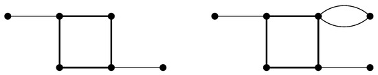Figure 2. Two available frames.

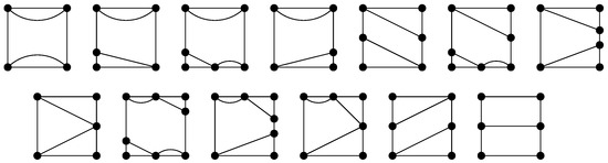Figure 3. Thirteen available pictures to insert into a frame.

4.

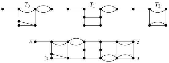
The set $\mathcal{T}\left(\mathcal{S}\right)$ consists of all graphs of the form $\circ \left({(\otimes \mathcal{T})}^{\updownarrow }\right)$, where $\mathcal{T}$ is a sequence $(T_0,{}^{\updownarrow }{T}_1^{\updownarrow },T_2,$$\dots ,{}^{\updownarrow }{T}_{2m-1}^{\updownarrow },T_{2m})$ such that $m\ge 1$ and $\forall i:$$T_i\in \mathcal{S}$.

Large 2-crossing-critical graphs are described in Item 1 of Theorem 3. Item 3 of Definition 9 describes the set of tiles (see Figure 4 for example) used in the construction of large 2-crossing-critical graphs as described in Item 4 (see Figure 5 for example).

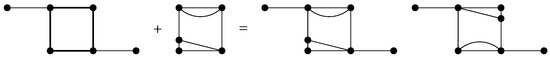
Figure 4. Demonstration of creation of tiles from $\mathcal{S}$.

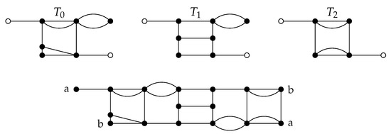
Figure 5. Example for $m=1$. For $\mathcal{T}=(T_0,T_1,T_2)$, $G=\circ \left({(\otimes \mathcal{T})}^{\updownarrow }\right)$ is shown. When appropriate white vertices are identified, they are suppressed (see [8] for details).

4.3. The Alphabet Describing Tiles

In [43], the reader can find an alphabet to describe tiles in large 2-crossing-critical graphs. There are four attributes that describe a tile:

• top path $P_t$: Describes the top path of the tile. $P_t\in \{D,A,V,B,H\}$ (see Figure 6 and Figure 7).
  

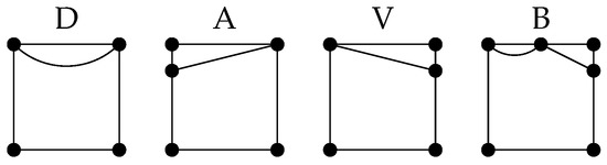  Figure 6. Alphabet letters describing top paths in tiles from $\mathcal{S}$.
  

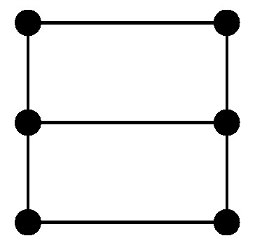  Figure 7. Additional letter H is used to describe one special picture. In this case, $P_t=H,Id=\varnothing ,P_b=\varnothing$.
• identification $Id$: Describes if top and bottom paths of the tile intersect. $Id\in \{I,\varnothing \}$ (see Figure 8).
  

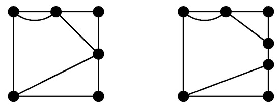  Figure 8. On the left side, $Id=I$; on the right side, $Id=\varnothing$.
• bottom path $P_b$: Describes the bottom path of the tile. $P_b\in \{D,A,V,B,\varnothing \}$ (see Figure 9).
  

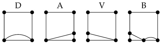  Figure 9. Alphabet letters describing bottom paths in tiles from $\mathcal{S}$.
• frame $Fr$: Describes the frame used for the tile. $Fr\in \{L,dL\}$ (see Figure 10).
  

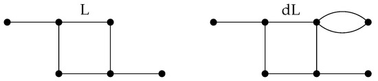  Figure 10. Alphabet letters describing frames.

Using this notation, each tile $T\in \mathcal{S}$ has its own signature:

$$sig\left(T\right)=P_{t}Id{P}_{b}Fr.$$

If some attribute is equal to ∅, it is omitted in the signature. For a graph $G\in \mathcal{T}\left(\mathcal{S}\right)$, $G=\circ \left({(\otimes \mathcal{T})}^{\updownarrow }\right)$, where $\mathcal{T}=(T_0,{}^{\updownarrow }{T}_1^{\updownarrow },T_2,\dots ,{}^{\updownarrow }{T}_{2m-1}^{\updownarrow },T_{2m})$, we introduce a signature in a natural way:

$$sig\left(G\right)=sig\left(T_0\right)sig\left(T_1\right)\dots sig\left(T_{2m-1}\right)sig\left(T_{2m}\right).$$

In connection with the introduced signature, we later use the following notation:

• for $X\in \{B,D,A,V,H,I,d\}$, #X is the number of occurrences of X in $sig\left(G\right)$;
• for $j\in \{0,1,\dots ,2m\}$ and $X\in \{B,D,A,V,H,I,d\}$, ${\#}_{j}X$ is the number of occurrences of X in $sig\left(T_j\right)$; and
• for $j\in \{0,1,\dots ,2m\}$, $p\in \{P_t,P_b\}$ and $X\in \{B,D,A,V\}$, ${\#}_j^{p}X$ is the number of occurrences of X as $sig{\left(T_j\right)}_p$.

5. Hamiltonian Cycles in Large 2-Crossing-Critical Graphs

In this section, we use the fact that large 2-crossing-critical graphs are a special case of 2-tiled graphs with a finite set of tiles to efficiently count Hamiltonian cycles with the use of algorithms from Section 3.

Remark 1.

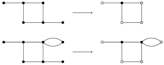
In the construction of large 2-crossing-critical graphs, degree one vertices of adjacent tiles that are to be identified are suppressed after identification so that there is no degree 2 vertex in G (see [8] for details and Figure 5 for example). Because of this, we define new types of frames, which are obtained from original frames by removing the tail of a frame (see Figure 11). We use these frames for constructing tiles in $\mathcal{S}$. Then, the cyclization of old tiles with additional suppression of a vertex is equivalent to the cyclization of new tiles (see Figure 12 for example). Note that all old graphs are the same as new ones, but the new tiles are not 2-degenerate; hence, for this method of construction of large 2-crossing-critical graphs, Theorem 2.18 from [8] does not yield 2-crossing-criticality. Each tile in a new set $\mathcal{S}$ is a 2-tile, and large 2-crossing-critical graphs are obtained by cyclization of at least three such 2-tiles. Therefore, by Definition 2, they are 2-tiled graphs. Because of that, we can use the algorithms from Section 3 to count Hamiltonian cycles (efficiently).

Figure 11. Transformation of frames. In transformed frames, white vertices are the left wall vertices and gray vertices are the right wall vertices of a 2-tile.

Figure 12. Graph G from Figure 5 can be obtained using modified tiles $T_0,T_1,T_2$. The signature of this graph is $sig\left(G\right)=DVdLHdLDDL$. Later in Example 1, we show that the total number of Hamiltonian cycles in G is 224.

Let

$$R=\left[\begin{array}{cc}{a}_{=}& a_{\times }\\ a_{\times }& a_{=}\end{array}\right]$$

and

$$Z=\left[\begin{array}{cccc}{a}_{{}_{\left\{{\overline{x}}_2\right\}}{-}_{\left\{y_2\right\}}}& a_{{}_{\left\{{\overline{x}}_1\right\}}{-}_{\left\{y_2\right\}}}& a_{{}_{\left\{x_2\right\}}{-}_{\left\{y_2\right\}}}& a_{{}_{\left\{x_1\right\}}{-}_{\left\{y_2\right\}}}\\ a_{{}_{\left\{{\overline{x}}_2\right\}}{-}_{\left\{y_1\right\}}}& a_{{}_{\left\{{\overline{x}}_1\right\}}{-}_{\left\{y_1\right\}}}& a_{{}_{\left\{x_2\right\}}{-}_{\left\{y_1\right\}}}& a_{{}_{\left\{x_1\right\}}{-}_{\left\{y_1\right\}}}\\ a_{{}_{\left\{{\overline{x}}_2\right\}}{-}_{\left\{{\overline{y}}_2\right\}}}& a_{{}_{\left\{{\overline{x}}_1\right\}}{-}_{\left\{{\overline{y}}_2\right\}}}& a_{{}_{\left\{x_2\right\}}{-}_{\left\{{\overline{y}}_2\right\}}}& a_{{}_{\left\{x_1\right\}}{-}_{\left\{{\overline{y}}_2\right\}}}\\ a_{{}_{\left\{{\overline{x}}_2\right\}}{-}_{\left\{{\overline{y}}_1\right\}}}& a_{{}_{\left\{{\overline{x}}_1\right\}}{-}_{\left\{{\overline{y}}_1\right\}}}& a_{{}_{\left\{x_2\right\}}{-}_{\left\{{\overline{y}}_1\right\}}}& a_{{}_{\left\{x_1\right\}}{-}_{\left\{{\overline{y}}_1\right\}}}\end{array}\right]$$

be matrices of tiles from $\mathcal{S}$ (R is from Equation (2) and Z from Equation (4)).

Remark 2.

In the construction of large 2-crossing-critical graphs, tiles at odd index (even index in algorithms) are inverted (see Item 4 of Definition 9). The matrices in the algorithms for such tiles (inverted ones) can be obtained from the original ones in time $\mathcal{O}\left(1\right)$:

$${}^{\updownarrow }{R}^{\updownarrow }=\left[\begin{array}{cc}{}^{\updownarrow }{a}_{=}^{\updownarrow }& {}^{\updownarrow }{a}_{\times }^{\updownarrow }\\ {}^{\updownarrow }{a}_{\times }^{\updownarrow }& {}^{\updownarrow }{a}_{=}^{\updownarrow }\end{array}\right]=\left[\begin{array}{cc}{a}_{=}& a_{\times }\\ a_{\times }& a_{=}\end{array}\right]=R,$$

$$\begin{array}{cc}\hfill {}^{\updownarrow }{Z}^{\updownarrow }& =\left[\begin{array}{cccc}{}^{\updownarrow }{a}_{{}_{\left\{{\overline{x}}_2\right\}}{-}_{\left\{y_2\right\}}}^{\updownarrow }& {}^{\updownarrow }{a}_{{}_{\left\{{\overline{x}}_1\right\}}{-}_{\left\{y_2\right\}}}^{\updownarrow }& {}^{\updownarrow }{a}_{{}_{\left\{x_2\right\}}{-}_{\left\{y_2\right\}}}^{\updownarrow }& {}^{\updownarrow }{a}_{{}_{\left\{x_1\right\}}{-}_{\left\{y_2\right\}}}^{\updownarrow }\\ {}^{\updownarrow }{a}_{{}_{\left\{{\overline{x}}_2\right\}}{-}_{\left\{y_1\right\}}}^{\updownarrow }& {}^{\updownarrow }{a}_{{}_{\left\{{\overline{x}}_1\right\}}{-}_{\left\{y_1\right\}}}^{\updownarrow }& {}^{\updownarrow }{a}_{{}_{\left\{x_2\right\}}{-}_{\left\{y_1\right\}}}^{\updownarrow }& {}^{\updownarrow }{a}_{{}_{\left\{x_1\right\}}{-}_{\left\{y_1\right\}}}^{\updownarrow }\\ {}^{\updownarrow }{a}_{{}_{\left\{{\overline{x}}_2\right\}}{-}_{\left\{{\overline{y}}_2\right\}}}^{\updownarrow }& {}^{\updownarrow }{a}_{{}_{\left\{{\overline{x}}_1\right\}}{-}_{\left\{{\overline{y}}_2\right\}}}^{\updownarrow }& {}^{\updownarrow }{a}_{{}_{\left\{x_2\right\}}{-}_{\left\{{\overline{y}}_2\right\}}}^{\updownarrow }& {}^{\updownarrow }{a}_{{}_{\left\{x_1\right\}}{-}_{\left\{{\overline{y}}_2\right\}}}^{\updownarrow }\\ {}^{\updownarrow }{a}_{{}_{\left\{{\overline{x}}_2\right\}}{-}_{\left\{{\overline{y}}_1\right\}}}^{\updownarrow }& {}^{\updownarrow }{a}_{{}_{\left\{{\overline{x}}_1\right\}}{-}_{\left\{{\overline{y}}_1\right\}}}^{\updownarrow }& {}^{\updownarrow }{a}_{{}_{\left\{x_2\right\}}{-}_{\left\{{\overline{y}}_1\right\}}}^{\updownarrow }& {}^{\updownarrow }{a}_{{}_{\left\{x_1\right\}}{-}_{\left\{{\overline{y}}_1\right\}}}^{\updownarrow }\end{array}\right]\hfill \\ \hfill & =\left[\begin{array}{cccc}{a}_{{}_{\left\{{\overline{x}}_1\right\}}{-}_{\left\{y_1\right\}}}& a_{{}_{\left\{{\overline{x}}_2\right\}}{-}_{\left\{y_1\right\}}}& a_{{}_{\left\{x_1\right\}}{-}_{\left\{y_1\right\}}}& a_{{}_{\left\{x_2\right\}}{-}_{\left\{y_1\right\}}}\\ a_{{}_{\left\{{\overline{x}}_1\right\}}{-}_{\left\{y_2\right\}}}& a_{{}_{\left\{{\overline{x}}_2\right\}}{-}_{\left\{y_2\right\}}}& a_{{}_{\left\{x_1\right\}}{-}_{\left\{y_2\right\}}}& a_{{}_{\left\{x_2\right\}}{-}_{\left\{y_2\right\}}}\\ a_{{}_{\left\{{\overline{x}}_1\right\}}{-}_{\left\{{\overline{y}}_1\right\}}}& a_{{}_{\left\{{\overline{x}}_2\right\}}{-}_{\left\{{\overline{y}}_1\right\}}}& a_{{}_{\left\{x_1\right\}}{-}_{\left\{{\overline{y}}_1\right\}}}& a_{{}_{\left\{x_2\right\}}{-}_{\left\{{\overline{y}}_1\right\}}}\\ a_{{}_{\left\{{\overline{x}}_1\right\}}{-}_{\left\{{\overline{y}}_2\right\}}}& a_{{}_{\left\{{\overline{x}}_2\right\}}{-}_{\left\{{\overline{y}}_2\right\}}}& a_{{}_{\left\{x_1\right\}}{-}_{\left\{{\overline{y}}_2\right\}}}& a_{{}_{\left\{x_2\right\}}{-}_{\left\{{\overline{y}}_2\right\}}}\end{array}\right]\hfill \\ \hfill & =\left[\begin{array}{cccc}0& 1& 0& 0\\ 1& 0& 0& 0\\ 0& 0& 0& 1\\ 0& 0& 1& 0\end{array}\right]·Z·\left[\begin{array}{cccc}0& 1& 0& 0\\ 1& 0& 0& 0\\ 0& 0& 0& 1\\ 0& 0& 1& 0\end{array}\right]\hfill \\ \hfill & =X·Z·X.\hfill \end{array}$$

Remark 3.

In the construction of large 2-crossing-critical graphs, there is a twist in connecting the last and the first tiles (see Item 4 of Definition 9).

The matrices in the algorithms for the last tile (the right-inverted one) can be obtained from the original one in time $\mathcal{O}\left(1\right)$:

$$R^{\updownarrow }=\left[\begin{array}{cc}{a}_{=}^{\updownarrow }& a_{\times }^{\updownarrow }\\ a_{\times }^{\updownarrow }& a_{=}^{\updownarrow }\end{array}\right]=\left[\begin{array}{cc}{a}_{\times }& a_{=}\\ a_{=}& a_{\times }\end{array}\right]=\left[\begin{array}{cc}0& 1\\ 1& 0\end{array}\right]·R,$$

$$\begin{array}{cc}\hfill Z^{\updownarrow }& =\left[\begin{array}{cccc}{a}_{{}_{\left\{{\overline{x}}_2\right\}}{-}_{\left\{y_2\right\}}}^{\updownarrow }& a_{{}_{\left\{{\overline{x}}_1\right\}}{-}_{\left\{y_2\right\}}}^{\updownarrow }& a_{{}_{\left\{x_2\right\}}{-}_{\left\{y_2\right\}}}^{\updownarrow }& a_{{}_{\left\{x_1\right\}}{-}_{\left\{y_2\right\}}}^{\updownarrow }\\ a_{{}_{\left\{{\overline{x}}_2\right\}}{-}_{\left\{y_1\right\}}}^{\updownarrow }& a_{{}_{\left\{{\overline{x}}_1\right\}}{-}_{\left\{y_1\right\}}}^{\updownarrow }& a_{{}_{\left\{x_2\right\}}{-}_{\left\{y_1\right\}}}^{\updownarrow }& a_{{}_{\left\{x_1\right\}}{-}_{\left\{y_1\right\}}}^{\updownarrow }\\ a_{{}_{\left\{{\overline{x}}_2\right\}}{-}_{\left\{{\overline{y}}_2\right\}}}^{\updownarrow }& a_{{}_{\left\{{\overline{x}}_1\right\}}{-}_{\left\{{\overline{y}}_2\right\}}}^{\updownarrow }& a_{{}_{\left\{x_2\right\}}{-}_{\left\{{\overline{y}}_2\right\}}}^{\updownarrow }& a_{{}_{\left\{x_1\right\}}{-}_{\left\{{\overline{y}}_2\right\}}}^{\updownarrow }\\ a_{{}_{\left\{{\overline{x}}_2\right\}}{-}_{\left\{{\overline{y}}_1\right\}}}^{\updownarrow }& a_{{}_{\left\{{\overline{x}}_1\right\}}{-}_{\left\{{\overline{y}}_1\right\}}}^{\updownarrow }& a_{{}_{\left\{x_2\right\}}{-}_{\left\{{\overline{y}}_1\right\}}}^{\updownarrow }& a_{{}_{\left\{x_1\right\}}{-}_{\left\{{\overline{y}}_1\right\}}}^{\updownarrow }\end{array}\right]\hfill \\ \hfill & =\left[\begin{array}{cccc}{a}_{{}_{\left\{{\overline{x}}_2\right\}}{-}_{\left\{y_1\right\}}}& a_{{}_{\left\{{\overline{x}}_1\right\}}{-}_{\left\{y_1\right\}}}& a_{{}_{\left\{x_2\right\}}{-}_{\left\{y_1\right\}}}& a_{{}_{\left\{x_1\right\}}{-}_{\left\{y_1\right\}}}\\ a_{{}_{\left\{{\overline{x}}_2\right\}}{-}_{\left\{y2\right\}}}& a_{{}_{\left\{{\overline{x}}_1\right\}}{-}_{\left\{y_2\right\}}}& a_{{}_{\left\{x_2\right\}}{-}_{\left\{y_2\right\}}}& a_{{}_{\left\{x_1\right\}}{-}_{\left\{y_2\right\}}}\\ a_{{}_{\left\{{\overline{x}}_2\right\}}{-}_{\left\{{\overline{y}}_1\right\}}}& a_{{}_{\left\{{\overline{x}}_1\right\}}{-}_{\left\{{\overline{y}}_1\right\}}}& a_{{}_{\left\{x_2\right\}}{-}_{\left\{{\overline{y}}_1\right\}}}& a_{{}_{\left\{x_1\right\}}{-}_{\left\{{\overline{y}}_1\right\}}}\\ a_{{}_{\left\{{\overline{x}}_2\right\}}{-}_{\left\{{\overline{y}}_2\right\}}}& a_{{}_{\left\{{\overline{x}}_1\right\}}{-}_{\left\{{\overline{y}}_2\right\}}}& a_{{}_{\left\{x_2\right\}}{-}_{\left\{{\overline{y}}_2\right\}}}& a_{{}_{\left\{x_1\right\}}{-}_{\left\{{\overline{y}}_2\right\}}}\end{array}\right]\hfill \\ \hfill & =\left[\begin{array}{cccc}0& 1& 0& 0\\ 1& 0& 0& 0\\ 0& 0& 0& 1\\ 0& 0& 1& 0\end{array}\right]·Z\hfill \\ \hfill & =X·Z.\hfill \end{array}$$

Remark 4.

As the tiles in $\mathcal{S}$ are planar, none of them contain an intertwined pair of disjoint paths; hence, none of the tiles from the set $\mathcal{S}$ is of C-type ×. Using this observation with Remark 2 and Remark 3, we get that, for each tile in $\mathcal{S}$, the following holds:

$$R={}^{\updownarrow }{R}^{\updownarrow }=\left[\begin{array}{cc}{a}_{=}& 0\\ 0& a_{=}\end{array}\right]\mathrm{and}{R}^{\updownarrow }=\left[\begin{array}{cc}0& a_{=}\\ a_{=}& 0\end{array}\right].$$

Corollary 3.

Let $G\in \mathcal{T}\left(\mathcal{S}\right)$. The number of traversing Hamiltonian cycles in G is equal to

$$THC\left(G\right)=\prod _{i=1}^{2m+1}{a}_{=}^i,$$

where $a_{=}^i$ is the number of possibilities for $T_i$ to be of C-type =.

Proof. 

Using Remark 4 in Equation (2), for $i\in \{1,2,\dots ,2m\}$, we get

$$\begin{array}{cc}\hfill c^i& =a_{=}^i·I·c^{i-1}\hfill \\ \hfill & =a_{=}^i·c^{i-1}\hfill \end{array}$$

and

$$\begin{array}{cc}\hfill c^{2m+1}& =a_{=}^{2m+1}·\left[\begin{array}{cc}0& 1\\ 1& 0\end{array}\right]·c^{2m}.\hfill \end{array}$$

Then,

$$c^{2m+1}=a_{=}^{2m+1}·a_{=}^{2m}\cdots a_{=}^1·\left[\begin{array}{cc}0& 1\\ 1& 0\end{array}\right]\left[\begin{array}{c}1\\ 0\end{array}\right]=\left[\begin{array}{c}0\\ \prod _{i=1}^{2m+1}{a}_{=}^i\end{array}\right].$$

Hence,

$$THC\left(G\right)=\prod _{i=1}^{2m+1}{a}_{=}^i.$$

□

Corollary 4.

Let $G\in \mathcal{T}\left(\mathcal{S}\right)$. The number of traversing Hamiltonian cycles in G is equal to

$$THC\left(G\right)=2^{\#B+\#D+\#H+\#I+\#d}.$$

Proof. 

We have shown before that $THC\left(G\right)=\prod _{i=1}^{2m+1}{a}_{=}^i.$ Using the alphabet defined above, we notice that

$$a_{=}^i=2^{{\#}_{i}B+{\#}_{i}D+{\#}_{i}H+{\#}_{i}I+{\#}_{i}d}.$$

Then,

$$\begin{array}{cc}\hfill THC\left(G\right)& =\prod _{i=1}^{2m+1}{2}^{{\#}_{i}B+{\#}_{i}D+{\#}_{i}H+{\#}_{i}I+{\#}_{i}d}\hfill \\ \hfill & =2^{\left(\sum _{i=1}^{2m+1}{\#}_{i}B\right)+\left(\sum _{i=1}^{2m+1}{\#}_{i}D\right)+\left(\sum _{i=1}^{2m+1}{\#}_{i}H\right)+\left(\sum _{i=1}^{2m+1}{\#}_{i}I\right)+\left(\sum _{i=1}^{2m+1}{\#}_{i}d\right)}\hfill \\ \hfill & =2^{\#B+\#D+\#H+\#I+\#d}.\hfill \end{array}$$

□

Corollary 5.

Let $G\in \mathcal{T}\left(\mathcal{S}\right)$. The number of flanking Hamiltonian cycles in G is equal to

$$FHC\left(G\right)=THC\left(G\right)·\sum _{i=1}^{2m+1}\frac{a_{\Vert }^i·a_{=}^{i+1}+a_{\left]\right[}^{i,i+1}}{a_{=}^i·a_{=}^{i+1}},$$

where

• $THC\left(G\right)$ is the number of traversing Hamiltonian cycles in G,
• $a_{=}^i$ is the number of possibilities for $T_i$ to be of C-type =,
• $a_{\Vert }^i$ is the number of possibilities for $T_i$ to be of C-type ‖,
• $a_{\left]\right[}^{i,i+1}$ is the number of distinct possibilities for $T_i$ and $T_{i+1}$ to be of compatible flanking C-types of forms ${|}_{\{x,y\}}$ and ${}_{\{z,w\}}|$.

Proof. 

As shown in the proof of Lemma 5,

$$\begin{array}{cc}\hfill FHC\left(G\right)& =\sum _{i=1}^{2m+1}{a}_{\Vert }^i·(c_{even}^{i+1,i-1}+c_{odd}^{i+1,i-1})+\sum _{i=1}^{2m+1}{a}_{\left]\right[}^{i,i+1}·(c_{even}^{i+2,i-1}+c_{odd}^{i+2,i-1})\hfill \\ & +\sum _{i=1}^{2m+1}{a}_{]\varnothing [}^{i,i+1,i+2}·(c_{even}^{i+3,i-1}+c_{odd}^{i+3,i-1}).\hfill \end{array}$$

Because each tile in $\mathcal{S}$ contains an internal vertex, for each tile in $\mathcal{S}$, the value $a_{\varnothing }=0$ (see the proof of Lemma 5). Hence, $\forall i\in \{1,2,\dots ,2m+1\},a_{]\varnothing [}^{i,i+1,i+2}=0$. Using Remark 4 as in the proof of Corollary 3, we get that

$$\left[\begin{array}{c}{c}_{even}^{i+1,i-1}\\ c_{odd}^{i+1,i-1}\end{array}\right]=\left[\begin{array}{c}0\\ \prod _{\begin{array}{c}j=1\\ j\ne i\end{array}}^{2m+1}{a}_{=}^j\end{array}\right]\mathrm{and}\left[\begin{array}{c}{c}_{even}^{i+2,i-1}\\ c_{odd}^{i+2,i-1}\end{array}\right]=\left[\begin{array}{c}0\\ {\displaystyle \prod _{\begin{array}{c}j=1\\ j\notin \{i,i+1\}\end{array}}^{2m+1}}{a}_{=}^j\end{array}\right].$$

It is easy to check that, for each tile in $\mathcal{S}$, the value $a_{=}>0$. Using observations and the result from the proof of Corollary 3 that $THC\left(G\right)=\prod _{j=1}^{2m+1}{a}_{=}^j$, we get

$$\begin{array}{cc}\hfill c_{odd}^{i+1,i-1}& =\prod _{\begin{array}{c}j=1\\ j\ne i\end{array}}^{2m+1}{a}_{=}^j=\frac{1}{a_{=}^i}\prod _{j=1}^{2m+1}{a}_{=}^j=\frac{1}{a_{=}^i}·THC\left(G\right),\hfill \\ \hfill c_{odd}^{i+2,i-1}& =\prod _{\begin{array}{c}j=1\\ j\notin \{i,i+1\}\end{array}}^{2m+1}{a}_{=}^j=\frac{1}{a_{=}^i·a_{=}^{i+1}}\prod _{j=1}^{2m+1}{a}_{=}^j=\frac{1}{a_{=}^i·a_{=}^{i+1}}·THC\left(G\right).\hfill \end{array}$$

Hence,

$$FHC\left(G\right)=THC\left(G\right)·\sum _{i=1}^{2m+1}\frac{a_{\Vert }^i·a_{=}^{i+1}+a_{\left]\right[}^{i,i+1}}{a_{=}^i·a_{=}^{i+1}}.$$

□

Corollary 6.

Let $G\in \mathcal{T}\left(\mathcal{S}\right)$. The number of flanking Hamiltonian cycles in G is equal to

$$FHC\left(G\right)=THC\left(G\right)·\sum _{i=1}^{2m+1}\frac{2^{{\#}_{i}d}·2^{{\#}_{i+1}B+{\#}_{i+1}D+{\#}_{i+1}H+{\#}_{i+1}I+{\#}_{i+1}d}+{\rm Y}(T_i,T_{i+1})}{2^{{\#}_{i}B+{\#}_{i}D+{\#}_{i}H+{\#}_{i}I+{\#}_{i}d}·2^{{\#}_{i+1}B+{\#}_{i+1}D+{\#}_{i+1}H+{\#}_{i+1}I+{\#}_{i+1}d}},$$

where

$${\rm Y}(T_i,T_{i+1})=\left\{\begin{array}{c}(1-{\#}_{i}H)·2^{{\#}_{i}B+{\#}_{i}D}·(1-{\#}_{i+1}H)·\hfill \\ ·2^{{\#}_{i+1}B+{\#}_{i+1}D+{\#}_{i+1}d};\hfill & \mathrm{if}sig{\left(T_i\right)}_{Fr}=dL\hfill \\ (1-{\#}_{i}H)·2^{{\#}_{i}B+{\#}_{i}D}·({\#}_{i+1}^{P_b}V·2^{{\#}_{i+1}^{P_t}B+{\#}_{i+1}^{P_t}D}+\hfill \\ +2·{\#}_{i+1}^{P_b}B·2^{{\#}_{i+1}^{P_t}B+{\#}_{i+1}^{P_t}D}+{\#}_{i+1}^{P_t}V·\hfill \\ ·(1-{\#}_{i+1}^{P_b}B)+{\#}_{i+1}H-{\#}_{i+1}^{P_b}V·{\#}_{i+1}^{P_t}V)·2^{{\#}_{i+1}d}+\hfill \\ +({\#}_i^{P_t}V·2^{{\#}_i^{P_b}B+{\#}_i^{P_b}D}+2·{\#}_i^{P_t}B·2^{{\#}_i^{P_b}B+{\#}_i^{P_b}D}+\hfill \\ +{\#}_i^{P_b}V·(1-{\#}_i^{P_t}B)+{\#}_{i}H-{\#}_i^{P_t}V·{\#}_i^{P_b}V)·\hfill \\ ·(1-{\#}_{i+1}H)·2^{{\#}_{i+1}B+{\#}_{i+1}D+{\#}_{i+1}d};\hfill & \mathrm{if}sig{\left(T_i\right)}_{Fr}=L\hfill \end{array}\right..$$

Note that the notation implies the number can be computed solely from the signature of a 2-crossing-critical graph. The structure of the equation is explained through the proof that follows.

Proof. 

We have shown in the proof of Corollary 4 that $a_{=}^i=2^{{\#}_{i}D+{\#}_{i}B+{\#}_{i}H+{\#}_{i}I+{\#}_{i}d}$. It is easy to see that

$$a_{\Vert }^i=\left\{\begin{array}{cc}2;\hfill & \mathrm{if}sig{\left(T_i\right)}_{Fr}=dL\hfill \\ 1;\hfill & \mathrm{if}sig{\left(T_i\right)}_{Fr}=L\hfill \end{array}\right.=2^{{\#}_{i}d}.$$

It remains to show that $a_{\left]\right[}^{i,i+1}={\rm Y}(T_i,T_{i+1})$:

1.

Let $sig{\left(T_i\right)}_{Fr}=dL$. Using Figure 13, it is easy to see that

$$a_{\left]\right[}^{i,i+1}=a_{{|}_{\{{\overline{y}}_1,y_2\}}}^i·a_{{}_{\{x_1,{\overline{x}}_2\}}|}^{i+1}.$$

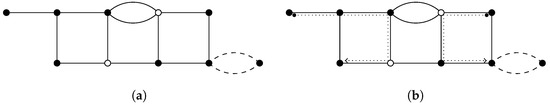Figure 13. (a) Drawing of $T_i\otimes {}^{\updownarrow }{T}_{i+1}^{\updownarrow }$, where $sig{\left(T_i\right)}_{Fr}=dL$. White vertices are right wall vertices of tile $T_i$ and left wall vertices of tile $T_{i+1}$. (b) Dotted arrows show the only possible combination for $a_{\left]\right[}^{i,i+1}$.

For $a_{{|}_{\{{\overline{y}}_1,y_2\}}}^i$, all pictures except H are valid, and paths B and D add a multiplier 2. Hence,

$$a_{{|}_{\{{\overline{y}}_1,y_2\}}}^i=(1-{\#}_{i}H)·2^{{\#}_{i}B+{\#}_{i}D}.$$

For $a_{{}_{\{x_1,{\overline{x}}_2\}}|}^{i+1}$, all pictures except H are valid, and paths B and D, and the frame $dL$ add a multiplier 2. Hence,

$$a_{{}_{\{x_1,{\overline{x}}_2\}}|}^{i+1}=(1-{\#}_{i+1}H)·2^{{\#}_{i+1}B+{\#}_{i+1}D+{\#}_{i+1}d}.$$

2.

Let $sig{\left(T_i\right)}_{Fr}=L$. Using Figure 14, it is easy to see that

$$a_{\left]\right[}^{i,i+1}=a_{{|}_{\{y_1,y_2\}}}^i·a_{{}_{\{{\overline{x}}_1,{\overline{x}}_2\}}|}^{i+1}+a_{{|}_{\{{\overline{y}}_1,y_2\}}}^i·a_{{}_{\{x_1,{\overline{x}}_2\}}|}^{i+1}.$$

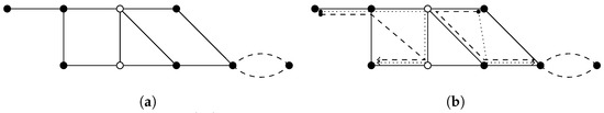Figure 14. (a) Drawing of $T_i\otimes {}^{\updownarrow }{T}_{i+1}^{\updownarrow }$, where $sig{\left(T_i\right)}_{Fr}=L$. White vertices are right wall vertices of tile $T_i$ and left wall vertices of tile $T_{i+1}$. (b) Dotted and dashed arrows show two possible combinations for $a_{\left]\right[}^{i,i+1}$.

For $a_{{|}_{\{y_1,y_2\}}}^i$, all pictures except H are valid, and paths B and D add a multiplier 2. Hence,

$$a_{{|}_{\{y_1,y_2\}}}^i=(1-{\#}_{i}H)·2^{{\#}_{i}B+{\#}_{i}D}.$$

For $a_{{}_{\{{\overline{x}}_1,{\overline{x}}_2\}}|}^{i+1}$, there are several options:

• The bottom path is V; the top path is any of the possible ones; and top paths B and D, and the frame $dL$ add a multiplier 2.
• The bottom path is B; the top path is any of the possible ones; and the bottom path B, top paths B and D, and the frame $dL$ add a multiplier 2.
• The top path is V; the bottom path is any of the possible ones, except B; and the frame $dL$ adds a multiplier 2.
• The top path is H, and the frame $dL$ adds a multiplier 2.

The first and the third options both cover the picture with the top path V and the bottom path V. Hence,

$$\begin{array}{cc}\hfill a_{{}_{\{{\overline{x}}_1,{\overline{x}}_2\}}|}^{i+1}& =({\#}_{i+1}^{P_b}V·2^{{\#}_{i+1}^{P_t}B+{\#}_{i+1}^{P_t}D}+2·{\#}_{i+1}^{P_b}B·2^{{\#}_{i+1}^{P_t}B+{\#}_{i+1}^{P_t}D}\hfill \\ & +{\#}_{i+1}^{P_t}V·(1-{\#}_{i+1}^{P_b}B)+{\#}_{i+1}H-{\#}_{i+1}^{P_b}V·{\#}_{i+1}^{P_t}V)·2^{{\#}_{i+1}d}.\hfill \end{array}$$

For $a_{{|}_{\{{\overline{y}}_1,y_2\}}}^i$, there are several options:

• The top path is V; the bottom path is any of the possible ones; and the bottom paths B and D add a multiplier 2.
• The top path is B; the bottom path is any of the possible ones; and the top path B and bottom paths B and D add a multiplier 2.
• The bottom path is V, and the top path is any of the possible ones, except B.
• The top path is H.

The first and the third options both cover the picture with top path V and bottom path V. Hence,

$$\begin{array}{cc}\hfill a_{{|}_{\{{\overline{y}}_1,y_2\}}}^i& ={\#}_i^{P_t}V·2^{{\#}_i^{P_b}B+{\#}_i^{P_b}D}+2·{\#}_i^{P_t}B·2^{{\#}_i^{P_b}B+{\#}_i^{P_b}D}\hfill \\ & +{\#}_i^{P_b}V·(1-{\#}_i^{P_t}B)+{\#}_{i}H-{\#}_i^{P_t}V·{\#}_i^{P_b}V.\hfill \end{array}$$

For $a_{{}_{\{x_1,{\overline{x}}_2\}}|}^{i+1}$, all pictures except H are valid, and paths B and D, and the frame $dL$ add a multiplier 2. Hence,

$$a_{{}_{\{x_1,{\overline{x}}_2\}}|}^{i+1}=(1-{\#}_{i+1}H)·2^{{\#}_{i+1}B+{\#}_{i+1}D+{\#}_{i+1}d}.$$

□

Corollary 7.

Let $G\in \mathcal{T}\left(\mathcal{S}\right)$. The number of zigzagging Hamiltonian cycles in G is bounded by

$$0\le ZHC\left(G\right)\le 8^{2m+1}.$$

Proof. 

To count zigzagging Hamiltonian cycles, the algorithm from the proof of Lemma 6 with a slight difference (explained in Remark 2 and Remark 3) is used:

$$\begin{array}{cc}\hfill ZHC\left(G\right)& =tr(Z_{2m+1}^{\updownarrow }·{}^{\updownarrow }{Z}_{2m}^{\updownarrow }·Z_{2m-1}\cdots Z_3·{}^{\updownarrow }{Z}_2^{\updownarrow }·Z_1)\hfill \\ \hfill & =tr(\left(X·Z_{2m+1}\right)·\left(X·Z_{2m}·X\right)·Z_{2m-1}\cdots Z_3·\left(X·Z_2·X\right)·Z_1)\hfill \\ \hfill & =tr(\left(X·Z_{2m+1}\right)·\left(X·Z_{2m}\right)·\left(X·Z_{2m-1}\right)\cdots \left(X·Z_2\right)·\left(X·Z_1\right)),\hfill \end{array}$$

(5)

where X is the matrix from Remark 3.

The lower bound is achieved by a graph $G\in \mathcal{T}\left(\mathcal{S}\right)$, where $\forall i\in \{1,2,\dots ,2m+1\}:sig\left(T_i\right)=DDdL$. In this case, the matrices $Z_i$ are the following:

$$Z_i=\left[\begin{array}{cccc}0& 0& 4& 0\\ 0& 0& 0& 0\\ 4& 4& 0& 0\\ 2& 2& 0& 0\end{array}\right].$$

Hence,

$$X·Z_i=\left[\begin{array}{cccc}0& 0& 0& 0\\ 0& 0& 4& 0\\ 2& 2& 0& 0\\ 4& 4& 0& 0\end{array}\right].$$

Then,

$$\left(X·Z_{2m+1}\right)·\left(X·Z_{2m}\right)·\left(X·Z_{2m-1}\right)\cdots \left(X·Z_2\right)·\left(X·Z_1\right)=\left[\begin{array}{cccc}0& 0& 0& 0\\ 0& 0& 4·8^m& 0\\ 2·8^m& 2·8^m& 0& 0\\ 4·8^m& 4·8^m& 0& 0\end{array}\right]$$

and

$$ZHC\left(G\right)=tr(\left(X·Z_{2m+1}\right)·\left(X·Z_{2m}\right)·\left(X·Z_{2m-1}\right)\cdots \left(X·Z_2\right)·\left(X·Z_1\right))=0.$$

We now study the upper bound for the number of zigzagging Hamiltonian cycles.

Remark 5.

For matrices $X,Y\in M_n\left({\mathbb{R}}_0^{+}\right)$, let the coefficient $K(X,Y)$ be defined as

$$\begin{array}{cc}\hfill K(X,Y)& =n-({\#}_{\mathrm{zero}\mathrm{columns}\mathrm{in}X}+{\#}_{\mathrm{zero}\mathrm{rows}\mathrm{in}Y}\hfill \\ & -{\#}_{\mathrm{of}\mathrm{indices}i\mathrm{so}\mathrm{that}\mathrm{the}{X}^i\mathrm{column}\mathrm{and}{Y}_i\mathrm{row}\mathrm{are}\mathrm{both}\mathrm{zero}}).\hfill \end{array}$$

If $UB\left(X\right)$ and $UB\left(Y\right)$ are the upper bounds for elements in matrices X and Y, then

$$UB\left(X·Y\right)=K(X,Y)·UB\left(X\right)·UB\left(Y\right)$$

is an upper bound for elements in matrix $X·Y$ (this is a direct corollary of the definition of matrix multiplication).

Based on the frame, we get the following two types of matrices:

• Tile with frame L:

  $$Z_L=\left[\begin{array}{cccc}{a}_{11}& a_{12}& a_{13}& 0\\ a_{21}& a_{22}& a_{23}& 0\\ a_{31}& a_{32}& a_{33}& 0\\ a_{41}& a_{42}& a_{43}& 0\end{array}\right],$$

  where $a_{ij}\le 2$ (frame adds a factor 1 and pictures add a factor 2).
• Tile with frame $dL$:

  $$Z_{dL}=\left[\begin{array}{cccc}{a}_{11}& a_{12}& a_{13}& 0\\ 0& 0& 0& 0\\ a_{31}& a_{32}& a_{33}& 0\\ a_{41}& a_{42}& a_{43}& 0\end{array}\right],$$

  where $a_{ij}\le 4$ (frame adds a factor 2 and pictures add a factor 2).

If we use the observation (5), we have two types of matrices in the product:

• Tile with frame L:

  $$X·Z_L=\left[\begin{array}{cccc}{a}_{21}& a_{22}& a_{23}& 0\\ a_{11}& a_{22}& a_{13}& 0\\ a_{41}& a_{42}& a_{43}& 0\\ a_{31}& a_{32}& a_{33}& 0\end{array}\right],$$

  where $a_{ij}\le 2$ and so $UB\left(X·Z_L\right)=2$.
• Tile with frame $dL$:

  $$X·Z_{dL}=\left[\begin{array}{cccc}0& 0& 0& 0\\ a_{11}& a_{12}& a_{13}& 0\\ a_{41}& a_{42}& a_{43}& 0\\ a_{31}& a_{32}& a_{33}& 0\end{array}\right],$$

  where $a_{ij}\le 4$ and so $UB\left(X·Z_{dL}\right)=4$.

We introduce two types of matrices:

$$R_1=\left[\begin{array}{cccc}*& *& *& 0\\ *& *& *& 0\\ *& *& *& 0\\ *& *& *& 0\end{array}\right]\mathrm{and}{R}_2=\left[\begin{array}{cccc}0& 0& 0& 0\\ *& *& *& 0\\ *& *& *& 0\\ *& *& *& 0\end{array}\right].$$

Remark 6.

It is obvious that $X·Z_L$ is of type $R_1$ and that $X·Z_{dL}$ is of type $R_2$.

For their product, the following holds:

$$\begin{array}{cc}\hfill R_1·R_1& \mathrm{is}\mathrm{of}\mathrm{type}{R}_1,\hfill \\ \hfill R_1·R_2& \mathrm{is}\mathrm{of}\mathrm{type}{R}_1,\hfill \\ \hfill R_2·R_1& \mathrm{is}\mathrm{of}\mathrm{type}{R}_2,\hfill \\ \hfill R_2·R_2& \mathrm{is}\mathrm{of}\mathrm{type}{R}_2.\hfill \end{array}$$

(6)

For coefficient defined in Remark 5, the following holds:

$$\begin{array}{cc}\hfill K(R_1,R_1)& =3,\hfill \\ \hfill K(R_1,R_2)& =2,\hfill \\ \hfill K(R_2,R_1)& =3,\hfill \\ \hfill K(R_2,R_2)& =2.\hfill \end{array}$$

(7)

Using Remark 6 and observations (6) and (7), we get the following combinations:

$$\begin{array}{c}\hfill UB\left(\left(X·Z_L\right)·\left(X·Z_L\right)\right)=3·2·2=12,\\ \hfill UB\left(\left(X·Z_{dL}\right)·\left(X·Z_L\right)\right)=3·4·2=24,\\ \hfill UB\left(\left(X·Z_L\right)·\left(X·Z_{dL}\right)\right)=2·2·2=8,\\ \hfill UB\left(\left(X·Z_{dL}\right)·\left(X·Z_{dL}\right)\right)=2·4·4=32.\end{array}$$

It is easy to check that we get the largest bound by using a combination with all components of the product (5) equal to $Z=X·Z_{dL}$. Then,

$$\begin{array}{cc}\hfill UB\left(Z^2\right)& =K(Z,Z)·UB\left(Z\right)·UB\left(Z\right)=2·UB{\left(Z\right)}^2\hfill \\ \hfill UB\left(Z^3\right)& =K(Z,Z^2)·UB\left(Z\right)·UB\left(Z^2\right)=2·UB\left(Z\right)·2·UB{\left(Z\right)}^2=2^2·UB{\left(Z\right)}^3\hfill \\ \hfill & ⋮\hfill \\ \hfill UB\left(Z^{2m+1}\right)& =K(Z,Z^{2m})·UB\left(Z\right)·UB\left(Z^{2m}\right)=2·UB\left(Z\right)·2^{2m-1}·UB{\left(Z\right)}^{2m}\hfill \\ & =2^{2m}·UB{\left(Z\right)}^{2m+1}.\hfill \end{array}$$

Because $UB\left(Z\right)=4$, we get

$$UB\left(Z^{2m+1}\right)=2^{2m}·4^{2m+1}.$$

Because $Z^{2m+1}$ is of type $R_2$, we get that

$$ZHC\left(G\right)\le ZHC\left(Z^{2m+1}\right)=tr\left(Z^{2m+1}\right)=2·UB\left(Z^{2m+1}\right)=2·2^{2m}·4^{2m+1}=8^{2m+1}.$$

□

Example 1.

We now compute the number of Hamiltonian cycles for the graph from Figure 12:

$$\begin{array}{cc}\hfill THC\left(G\right)& =\prod _{i=0}^2{a}_{=}^i\hfill \\ \hfill & =4·4·4\hfill \\ \hfill & =64,\hfill \\ \hfill FHC\left(G\right)& =THC\left(G\right)·\sum _{i=0}^2\frac{a_{\Vert }^i·a_{=}^{i+1}+a_{\left]\right[}^{i,i+1}}{a_{=}^i·a_{=}^{i+1}}\hfill \\ \hfill & =64·\left(\frac{2·4+0}{4·4}+\frac{2·4+0}{4·4}+\frac{1·4+16}{4·4}\right)\hfill \\ \hfill & =144,\hfill \\ \hfill ZHC\left(G\right)& =tr\left(\left(X·Z_2\right)·\left(X·Z_1\right)·\left(X·Z_0\right)\right)\hfill \\ \hfill & =16,\hfill \end{array}$$

because

$$\begin{array}{c}\hfill Z_0=\left[\begin{array}{cccc}2& 0& 2& 0\\ 0& 0& 0& 0\\ 0& 4& 0& 0\\ 0& 2& 0& 0\end{array}\right],Z_1=\left[\begin{array}{cccc}0& 2& 2& 0\\ 0& 0& 0& 0\\ 2& 0& 0& 0\\ 0& 1& 1& 0\end{array}\right],Z_2=\left[\begin{array}{cccc}0& 0& 2& 0\\ 2& 2& 0& 0\\ 2& 2& 0& 0\\ 0& 0& 2& 0\end{array}\right]\end{array}$$

and so

$$\begin{array}{cc}\hfill \left(X·Z_2\right)·\left(X·Z_1\right)·\left(X·Z_0\right)& =\left[\begin{array}{cccc}8& 8& 8& 0\\ 4& 4& 4& 0\\ 4& 4& 4& 0\\ 8& 8& 8& 0\end{array}\right].\hfill \end{array}$$

References

- Kuratowski, C. Sur le probleme des courbes gauches en Topologie. Fundam. Math. 1930, 15, 271–283. [Google Scholar] [CrossRef]
- Bollobas, B. Combinatorics: Set Systems, Hypergraphs, Families of Vectors and Probabilistic Combinatorics; Cambridge University Press: New York, NY, USA, 1986. [Google Scholar]
- Trotter, W.T., Jr.; Moore, J.I., Jr. Characterization problems for graphs, partially ordered sets, lattices, and families of sets. Discret. Math. 1976, 16, 361–381. [Google Scholar] [CrossRef]
- Chudnovsky, M.; Robertson, N.; Seymour, P.; Thomas, R. The strong perfect graph theorem. Ann. Math. 2006, 164, 51–229. [Google Scholar] [CrossRef]
- Lovász, L. A characterization of perfect graphs. J. Comb. Theory Ser. B 1972, 13, 95–98. [Google Scholar] [CrossRef]
- Archdeacon, D. A Kuratowski theorem for the projective plane. J. Graph Theory 1981, 5, 243–246. [Google Scholar] [CrossRef]
- Robertson, N.; Seymour, P.D. Graph minors. VIII. A Kuratowski theorem for general surfaces. J. Comb. Theory, Ser. B 1990, 48, 255–288. [Google Scholar] [CrossRef]
- Bokal, D.; Oporowski, B.; Richter, R.B.; Salazar, G. Characterizing 2-crossing-critical graphs. Adv. Appl. Math. 2016, 74, 23–208. [Google Scholar] [CrossRef]
- des Cloizeaux, J.; Jannik, G. Polymers in Solution: Their Modelling and Structure; Clarendon Press: Oxford, MS, USA, 1990. [Google Scholar]
- Bašić, N.; Bokal, D.; Boothby, T.; Rus, J. An algebraic approach to enumerating non-equivalent double traces in graphs. MATCH Commun. Math. Comput. Chem. 2017, 78, 581–594. [Google Scholar]
- Gradišar, H.; Božič, S.; Doles, T.; Vengust, D.; Hafner-Bratkovič, I.; Mertelj, A.; Webb, B.; Šali, A.; Klavžar, S.; Jerala, R. Design of a single-chain polypeptide tetrahedron assembled from coiled-coil segments. Nat. Chem. Biol. 2013, 9, 362–366. [Google Scholar] [CrossRef] [PubMed]
- Tošić, R.; Bodroža-Pantić, O.; Kwong, Y.H.H.; Straight, H.J. On the number of Hamiltonian cycles of P4 × Pn. Indian J. Pure Appl. Math. 1990, 21, 403–409. [Google Scholar]
- Kwong, Y.H.H.; Rogers, D.G. A matrix method for counting Hamiltonian cycles on grid graphs. Eur. J. Comb. 1994, 15, 277–283. [Google Scholar] [CrossRef][Green Version]
- Bodroža-Pantić, O.; Tošič, R. On the number of 2-factors in rectangular lattice graphs. Publ. De L’Institut Math. 1994, 56, 23–33. [Google Scholar]
- Stoyan, R.; Strehl, V. Enumeration of Hamiltonian circuits in rectangular grids. J. Comb. Math. Comb. Comput. 1996, 21, 109–127. [Google Scholar]
- Bodroža-Pantić, O.; Kwong, H.; Doroslovački, R.; Pantić, M. Enumeration of Hamiltonian cycles on a thick grid cylinder—Part I: Non-contractible Hamiltonian cycles. Appl. Anal. Discret. Math. 2019, 13, 28–60. [Google Scholar] [CrossRef]
- Bodroža-Pantić, O.; Pantić, B.; Pantić, I.; Bodroža-Solarov, M. Enumeration of Hamiltonian cycles in some grid graphs. MATCH Commun. Math. Comput. Chem. 2013, 70, 181–204. [Google Scholar]
- Higuchi, S. Field theoretic approach to the counting problem of Hamiltonian cycles of graphs. Phys. Rev. E 1998, 58, 128–132. [Google Scholar] [CrossRef]
- Higuchi, S. Counting Hamiltonian cycles on planar random lattices. Mod. Phys. Lett. A 1998, 13, 727–733. [Google Scholar] [CrossRef]
- Frieze, A.; Jerrum, M.; Molloy, M.; Robinson, R.; Worml, N. Generating and counting Hamilton cycles in random regular graphs. J. Algorithms 1996, 21, 176–198. [Google Scholar] [CrossRef]
- Fallon, J.E. Two Results in Drawing Graphs on Surfaces. Doctoral Dissertation, Louisiana State University and Agricultural and Mechanical College, Baton Rouge, LA, USA, 2018. retrived from LSU Digital Commons. [Google Scholar]
- Goodman, S.; Hedetniemi, S. Sufficient conditions for a graph to be Hamiltonian. J. Comb. Theory Ser. B 1974, 16, 175–180. [Google Scholar] [CrossRef]
- Faudree, R.J.; Gould, R.J. Characterizing forbidden pairs for Hamiltonian properties. Discret. Math. 1997, 173, 45–60. [Google Scholar] [CrossRef]
- Faudree, R.J.; Gould, R.; Jacobson, M. Forbidden triples implying Hamiltonicity: For all graphs. Discuss. Math. Graph Theory 2004, 24, 47–54. [Google Scholar] [CrossRef]
- Gagarin, A.; Myrvold, W.; Chambers, J. Forbidden minors and subdivisions for toroidal graphs with no K3,3’s. Electron. Notes Discret. Math. 2005, 22, 151–156. [Google Scholar] [CrossRef]
- Mohar, B. A linear time algorithm for embedding graphs in an arbitrary surface. SIAM J. Discret. Math. 1999, 12, 6–26. [Google Scholar] [CrossRef]
- Kawarabayashi, K.; Mohar, B.; Reed, B. A simpler linear time algorithm for embedding graphs into an arbitrary surface and the genus of graphs of bounded tree-width. In Proceedings of the 49th Annual IEEE Symposium on Foundations of Computer Science, Philadelphia, PA, USA, 23–25 October 2008; pp. 771–780. [Google Scholar]
- Chartr, G.; Geller, D.; Hedetniemi, S. Graphs with forbidden subgraphs. J. Comb. Theory Ser. B 1971, 10, 12–41. [Google Scholar] [CrossRef]
- Dvořák, Z. On forbidden subdivision characterizations of graph classes. Eur. J. Comb. 2008, 29, 1321–1332. [Google Scholar] [CrossRef]
- Šiřan, J. Infinite families of crossing-critical graphs with a given crossing number. Discret. Math. 1984, 48, 129–132. [Google Scholar] [CrossRef][Green Version]
- Kochol, M. Construction of crossing-critical graphs. Discret. Math. 1987, 66, 311–313. [Google Scholar] [CrossRef]
- Pinontoan, B.; Richter, R.B. Crossing numbers of sequence of graphs I: General tiles. Aust. J. Comb. 2004, 30, 197–206. [Google Scholar]
- Szalazar, G. Infinite families of crossing-critical graphs with given average degree. Discret. Math. 2003, 271, 343–350. [Google Scholar] [CrossRef]
- Hlineny, P. New infinite families of almost-planar crossing-critical graphs. Electron. J. Comb. 2008, 15, R102:1–12. [Google Scholar]
- Bokal, D.; Bračič, M.; Derňár, M.; Hliněný, P. On degree properties of crossing-critical families of graphs. Electron. J. Comb. 2019, 26, P153:1–28. [Google Scholar] [CrossRef]
- Dvořák, Z.; Hliněný, P.; Mohar, B. Structure and generation of crossing-critical graphs. In Proceedings of the 34th International Symposium on Computational Geometry, Budapest, Hungary, 11–14 June 2018; pp. 33:1–33:14. [Google Scholar]
- Bokal, D.; Dvořák, Z.; Hliněný, P.; Leanos, J.; Mohar, B.; Wiedera, T. Bounded degree conjecture holds precisely for c-crossing-critical graphs with c≤12. In Proceedings of the 35th International Symposium on Computational Geometry, Portland, OR, USA, 18–21 June 2019; pp. 14:1–14:15. [Google Scholar]
- Dvořák, Z.; Mohar, M. Crossing-critical graphs with large maximum degree. J. Comb. Theory Ser. B 2010, 100, 413–417. [Google Scholar] [CrossRef]
- Dvořák, Z.; Mohar, M. Crossing numbers of periodic graphs. J. Graph Theory 2015, 83, 34–43. [Google Scholar] [CrossRef]
- Bokal, D.; Chimani, M.; Nover, A.; Schierbaum, J.; Stolzmann, T.; Wagner, M.H.; Wiedera, T. Invariants in large 2-crossing-critical graphs. J. Graph Algorithms Appl. under review.
- Lovász, L. Large Networks and Graph Limits; American Mathematical Society: Providence, RI, USA, 2012. [Google Scholar]
- Bokal, D. Infinite families of crossing-critical graphs with prescribed average degree and crossing number. J. Graph Theory 2010, 65, 139–162. [Google Scholar] [CrossRef]
- Žerak, T.; Bokal, D. Playful introduction to 2-crossing-critical graphs. Dianoia 2019, 3, 101–108. [Google Scholar]
Publisher’s Note: MDPI stays neutral with regard to jurisdictional claims in published maps and institutional affiliations. |
© 2021 by the authors. Licensee MDPI, Basel, Switzerland. This article is an open access article distributed under the terms and conditions of the Creative Commons Attribution (CC BY) license (http://creativecommons.org/licenses/by/4.0/).