Fractal Stochastic Processes on Thin Cantor-Like Sets

Abstract

We review the basics of fractal calculus, define fractal Fourier transformation on thin Cantor-like sets and introduce fractal versions of Brownian motion and fractional Brownian motion. Fractional Brownian motion on thin Cantor-like sets is defined with the use of non-local fractal derivatives. The fractal Hurst exponent is suggested, and its relation with the order of non-local fractal derivatives is established. We relate the Gangal fractal derivative defined on a one-dimensional stochastic fractal to the fractional derivative after an averaging procedure over the ensemble of random realizations. That means the fractal derivative is the progenitor of the fractional derivative, which arises if we deal with a certain stochastic fractal.

1. Introduction

Fractal geometry appears in many phenomena in nature [1,2,3,4,5,6]. The methods of ordinary integral and differential calculus are not effective or are inapplicable to the description of processes on fractals due to the irregular self-similar geometry with a fractal dimension exceeding the fractal’s topological dimension [7,8,9,10,11]. Sometimes, equations with derivatives and integrals of fractional orders are used to describe processes on fractal structures [12]. However, it should be noted that the relationship between fractals and fractional calculus is not evident, often artificial and criticized in some works [13]. In any case, the matter is not complete without introducing additional procedures, for example, averaging over realizations of random fractals [14,15,16]. A relation of fractional time derivatives to the continuous time random walk theory with fractal time behavior is presented in [14] and utilized in many works (see, e.g., [17,18,19]).

On the other hand, in the seminal paper of Gangal, fractal calculus was formulated via generalization of the Riemann method and applied to the description of some physical problems. Fractal calculus has advantages [7,8,9,10,11,20,21,22,23,24,25] important for its application. It is algorithmic and applicable to deterministic fractals, and fractional order of arising differential or integral operators is directly related to the fractal dimensions of structures.

In this paper, we consider some aspects of stochastic processes defined on fractal sets. After a short review of the basics of fractal calculus and the definition of a fractal Fourier transformation on thin Cantor-like sets, we define Brownian motion and fractional Brownian motion on thin Cantor-like sets. Fractional Brownian motion on thin Cantor-like sets is defined via non-local fractal derivatives, stochastic processes, and fractal integrals. The fractal Hurst exponent is suggested, and its relation with the order of non-local fractal derivatives is also derived.

Additionally, we relate the Gangal fractal derivative defined on a one-sided stochastic fractal of time points to the fractional derivative after an averaging procedure over the ensemble of random realizations. The counting process defined on a corresponding fractal time set becomes the fractional Poisson process. In this case, the fractal derivative is the progenitor of the fractional derivative, which arises if we use a certain fractal distribution of events on the time axis.

2. Basic Tools

In References [7,8], calculus on fractal subsets of a real line was systematically developed. Here, we provide some basic definitions of the fractal calculus, which we use to “fractalize” stochastic processes.

2.1. Local Fractal Calculus

For some fractal set $\mathcal{K}\subset \mathbb{R}$, the flag function can be defined as follows [7]:

$$Q(\mathcal{K},J)=\left\{\begin{array}{c}1if\mathcal{K}\cap J\ne \varnothing \hfill \\ 0\mathrm{otherwise},\hfill \end{array}\right.$$

(1)

where $J=[b_1,b_2]$. Then, ${\rho }^{\alpha }[\mathcal{K},W]$ is given in [7,8,22] by

$${\rho }^{\alpha }[\mathcal{K},W]=\sum _{i=1}^n\mathsf{\Gamma }(\alpha +1){(t_i-t_{i-1})}^{\alpha }Q(\mathcal{K},[t_{i-1},t_i]),$$

where $W_{[b_1,b_2]}=\{b_1=t_0,t_1,t_2,\dots ,t_n=b_2\}$ is a subdivisions of J.

The mass function ${\gamma }^{\alpha }(\mathcal{K},b_1,b_2)$ is defined in [7,8,22] by

$${\gamma }^{\alpha }(\mathcal{K},b_1,b_2)=\underset{\delta \to 0}{lim}\left(\underset{W_{[b_1,b_2]}:\left|W\right|\le \delta }{inf}{\rho }^{\alpha }[\mathcal{K},W]\right).$$

(2)

The infimum in latter relation is evaluated over all subdivisions W of $[b_1,b_2]$ in a way that $\left|W\right|:={max}_{1\le i\le n}(t_i-t_{i-1})\le \delta$.

In [7,8,22], the integral staircase function is introduced $S_{\mathcal{K}}^{\alpha }\left(t\right)$ according to

$$S_{\mathcal{K}}^{\alpha }\left(t\right)=\left\{\begin{array}{c}{\gamma }^{\alpha }(\mathcal{K},b_0,t)\mathrm{if}t\ge b_0\hfill \\ -{\gamma }^{\alpha }(\mathcal{K},b_0,t)\mathrm{otherwise},\hfill \end{array}\right.$$

(3)

where $b_0$ is a fixed real number.

The γ-dimension of a set $\mathcal{K}\cap [b_1,b_2]$ is given by

$$\begin{array}{ccc}\hfill {dim}_{\gamma }(\mathcal{K}\cap [b_1,b_2])& =& inf\{\alpha :{\gamma }^{\alpha }(\mathcal{K},b_1,b_2)=0\}\hfill \\ & =& sup\{\alpha :{\gamma }^{\alpha }(\mathcal{K},b_1,b_2)=\infty \}.\hfill \end{array}$$

(4)

The ${\mathcal{K}}^{\alpha }$-limit of a function $g:\mathbb{R}\to \mathbb{R}$ is defined by the following:

$$\forall ϵ>0,\exists \delta >0z\in \mathcal{K}\mathrm{and}|z-t|<\delta \Rightarrow \left|g\right(z)-l|<ϵ.$$

(5)

If l exists, then

$$l={\mathcal{K}}_{-}^{\alpha }\underset{z\to t}{lim}g\left(z\right).$$

(6)

A function $g:\mathbb{R}\to \mathbb{R}$ is ${\mathcal{K}}^{\alpha }$-continuous, if

$$g\left(t\right)={\mathcal{K}}_{-}^{\alpha }\underset{z\to t}{lim}g\left(z\right).$$

(7)

The ${\mathcal{K}}^{\alpha }$-derivative of $g\left(t\right)$ at t is defined by [7]

$$D_{\mathcal{K}}^{\alpha }g\left(t\right)=\left\{\begin{array}{c}{\mathcal{K}}_{-}^{\alpha }\underset{z\to t}{lim}\frac{g\left(z\right)-g\left(t\right)}{S_{\mathcal{K}}^{\alpha }\left(z\right)-S_{\mathcal{K}}^{\alpha }\left(t\right)},\mathrm{if},t\in \mathcal{K},\hfill \\ 0,\mathrm{otherwise},\hfill \end{array}\right.$$

(8)

if the limit exists.

The ${\mathcal{K}}^{\alpha }$-integral of $g\left(t\right)$ on interval $J=[b_1,b_2]$ is defined in [7,8] and approximately given by

$$\begin{array}{c}\hfill I_{\mathcal{K}}^{\alpha }g\left(t\right)={\int }_{b_1}^{b_2}g\left(t\right)d_{\mathcal{K}}^{\alpha }t\approx \sum _{i=1}^{n}g\left(t_i\right)(S_{\mathcal{K}}^{\alpha }\left(t_i\right)-S_{\mathcal{K}}^{\alpha }\left(t_{i-1}\right)).\end{array}$$

(9)

We refer the reader to [7,8,22] for more details.

The characteristic function of set $\mathcal{K}$ is defined by

$${\chi }_{\mathcal{K}}(\alpha ,t)=\left\{\begin{array}{cc}\frac{1}{\mathsf{\Gamma }(\alpha +1)},\hfill & t\in \mathcal{K};\hfill \\ 0,\hfill & \mathrm{otherwise}.\hfill \end{array}\right.$$

(10)

The conjugacy between the fractal calculus and standard calculus can be illustrated by the following map [7,8,22]:

$$\begin{array}{ccc}f& \stackrel{FractalIntegral/FractalDervitives}{\to }& f^{\prime }\\ \mathsf{\Phi }\downarrow \phantom{\mathsf{\Phi }}& & {\mathsf{\Phi }}^{-1}\uparrow \phantom{{\mathsf{\Phi }}^{-1}}& & \\ \\ g& \stackrel{StandardIntegral/StandardDervitives}{\to }& g^{\prime }\end{array}$$

where $D_{\mathcal{K}}^{\alpha }={\mathsf{\Phi }}^{-1}D\mathsf{\Phi }$ and $I_{\mathcal{K}}^{\alpha }={\mathsf{\Phi }}^{-1}I\mathsf{\Phi }$. The proof is given in [7,8], which makes it easy to fractalize standard results.

2.2. The Thin Cantor-Like Sets

The thin Cantor-like sets/middle-b Cantor set are built in the following stages:

• From the middle of $I=[0,1]$, we take an open interval of length $0<b<1$:

  $$C_1^b=\left[0,\frac{1}{2}(1-b)\right]\cup \left[\frac{1}{2}(1+b),1\right].$$

  (11)
• Remove disjoint open intervals of length b from the middle of the remaining closed intervals. The resulting set is

  $$\begin{array}{cc}\hfill & C_2^b=\left[0,\frac{1}{4}{(1-b)}^2\right]\cup \left[\frac{1}{4}(1-b^2),\frac{1}{2}(1-b)\right]\cup \left[\frac{1}{2}(1+b),\frac{1}{2}\left((1+b)+\frac{1}{2}{(1-b)}^2\right)\right]\hfill \\ & \cup \left[\frac{1}{2}(1+b)\left(1+\frac{1}{2}(1-b)\right),1\right].\hfill \\ & ⋮\end{array}$$

  (12)
• Delete disjoint open intervals of length b from the middle of the remaining closed intervals of step $k-1$; then, we have

  $$C^b=\bigcap _{k=1}^{\infty }{C}_k^b.$$

  (13)

The Hausdorff dimension of the middle-b Cantor set is

$${dim}_H\left(C^b\right)=\frac{log2}{log2-log(1-b)}.$$

(14)

Needless to say, all definitions provided in the previous subsection can be applied to the middle-b Cantor set ($\mathcal{K}=C^b$). For more details, we refer the reader to [7,8,22].

3. Stochastic Lévy–Lorentz Gas and Fractal Time

Fractional derivatives in diffusion models often arise due to fractal properties of the stochastic media [14,16,17,18,26,27,28,29]. Fractal derivative can be introduced for each realization of this media, not only for the averaged system. The question arises whether the equations with Gangal fractal derivatives for individual realizations of this media will correspond to the transport equations with fractional derivatives for the effective medium. Consider the following case of set $\mathcal{K}$, the so-called stochastic Lévy–Lorentz gas [26,28].

The medium in this model is presented by points $\left\{X_j\right\}=...,X_{-2},X_{-1},X_0=0,X_1,X_2,...$ (atoms), randomly distributed over x-axis. Let distances $X_j-X_{j-1}=R_j$ between neighboring atoms be independent identically distributed random variables with a common distribution:

$$F\left(x\right)=\mathrm{P}\{R<x\}={\int }_0^{x}f\left(x\right)dx.$$

(15)

In such a medium, the random positions $X_j$ are correlated, and it is possible to separate the set $\left\{X_j\right\}$ into two independent sequences $X_1,X_2,...$ and $X_{-1},X_{-2},...$, which originated from a common initial point $X_0=0$. This model is known as the one-dimensional Lorentz gas [26].

The distribution of random number $N_{+}\left(x\right)$ of atoms in the interval $(0,x]$

$$W(n,x)\equiv \mathrm{P}\{N_{+}\left(x\right)=n\}=F_n\left(x\right)-F_{n+1}\left(x\right)$$

(16)

is defined via the n-fold convolution $F_{n+1}\left(x\right)={\int }_0^x{F}_n(x-y)dF\left(y\right)$. Here, $F_1\left(x\right)=F\left(x\right)$.

The distribution of $N_{-}\left(x\right)$ in $[-x,0)$ can be found in a similar way. For various distributions $F\left(x\right)$, we obtain statistical ensemble of different kinds. To obtain a stochastic medium with a fractal property, one can take a heavy-tailed distribution [28],

$$1-F\left(x\right)\sim \frac{A}{\mathsf{\Gamma }(1-\alpha )}{x}^{-\alpha },A>0,x\to \infty .$$

(17)

A statistically homogeneous medium is obtained if we take $\alpha >2$; the variance $\mathrm{Var}\left(R\right)$ of R is finite in this case. For $\alpha <2$, $\mathrm{Var}\left(R\right)$ is infinite, and we deal with a stochastic fractal medium called the Lévy–Lorentz gas [26,30]. In contrast with a homogeneous medium, stochastic fractals do not obey the property of being self-averaging. For more details, we refer the reader to [28] or Chapter 1 of the book [30].

Let the sequence of time points $\left\{T_j\right\}=T_1,T_2,T_3,...$ be built in the same manner as the sequence $X_1,X_2,X_3,...$ above, namely $0<T_1<T_2<T_3<...,$ and $T_1,T_2-T_1,T_3-T_2,...$ are mutually identically independent distribution (i.i.d.) random variables with a general distribution $Q\left(t\right)=\mathrm{P}\{T_{j+1}-T_j<t\}$.

Assuming in particular

$$1-Q\left(t\right)\sim \frac{B}{\mathsf{\Gamma }(1-\beta )}{t}^{-\beta },t\to \infty ,0<\beta <1,$$

(18)

we obtain

$$W(k,t)dk\sim g^{(\beta ,1)}\left({\tau }_k\right)d{\tau }_k=w(z,\beta )dz,$$

(19)

where

$${\tau }_k=t{c}_{\beta }{n}^{-1/\beta },z=k/⟨K\left(t\right)⟩,⟨K\left(t\right)⟩=\frac{1}{\mathsf{\Gamma }(1+\beta )}{(t/c_{\beta })}^{\beta }\equiv K_1{t}^{\beta }.$$

(20)

Thus, the times of jumps $T_1,T_2,T_3,...$ form a stochastic fractal set ${\mathcal{T}}^{\beta }$ on the time axis with fractal dimension $\beta$.

Hilfer [31] studied fractal time random walks with generalized Mittag–Leffler functions as waiting time densities. These densities are usually used in the so-called fractional Poisson process [19].

The master equation for the fractional Poisson process ($\beta \le 1$) can be written in the following form [29]:

$${}_0{\mathsf{D}}_t^{\beta }{p}_n\left(t\right)=\mu [p_{n-1}\left(t\right)-p_n\left(t\right)]+\frac{t^{-\beta }}{\mathsf{\Gamma }(1-\beta )}{\delta }_{n_0},0<\beta \le 1.$$

(21)

where ${}_0{\mathsf{D}}_t^{\beta }$ is the left-sided Riemann–Liouville.

The Poisson process on fractal sets was introduced in [20]. The corresponding master equation has the following form:

$$D_{\mathcal{K}}^{\alpha }{p}_n\left(t\right)=\mu [p_{n-1}\left(t\right)-p_n\left(t\right)]+{\delta }_{\mathcal{K}}\left(t\right){\delta }_{n_0},0<\alpha \le 1.$$

(22)

where ${\delta }_{\mathcal{K}}\left(t\right)$ is the delta function defined on the fractal set.

If we take $\mathcal{K}={\mathcal{T}}^{\beta }$, after averaging over the ensemble of random realizations, the fractal derivative is proportional to the so-called fractional Marshaud derivative:

$${\mathrm{M}}_{+}^{\beta }f=\underset{h\downarrow 0}{lim}\frac{\beta }{\mathsf{\Gamma }(1-\beta )}\underset{h}{\overset{\infty }{\int }}\frac{f\left(z\right)-f(z-s)}{s^{\beta +1}}ds,$$

(23)

which for quite well functions coincides with the left-sided Riemann–Liouville derivative of order $\beta$. Therefore, we arrive at Equation (21). Non-locality arises as a result of averaging the local operator over the correlated distribution of time points.

The Poisson process is simple but one of the most important random processes for applications. The most fundamental equations describing physical processes on a microscopic level are obtained under the axioms of the Poisson process. Dealing with complex macroscopic systems, another type of behavior can be observed including fractal behavior and/or the presence of memory.

For the random walk on the fractal Lévy–Lorentz gas with trapping atoms [30], we derived the following asymptotic ($t\to \infty$) equation with the Riemann–Liouville derivatives:

$${}_0{\mathsf{D}}_t^{\beta }p(x,t)=\theta C{}_0{\mathsf{D}}_x^{\alpha }p(x,t)+c_{\alpha }^{-\alpha }(C/2)(1-{\theta }^2){}_0{\mathsf{D}}_x^{2\alpha }p(x,t)+\delta \left(x\right)t^{-\beta }/\mathsf{\Gamma }(1-\beta ),0<\alpha ,\beta <1,$$

(24)

where $p(x,t)$ is a probability density function and $\theta$ is an asymmetry parameter.

Fractional derivatives in different models often arise due to fractal properties of systems (see, e.g., [12,14,16,29,31,32,33]). Here, we argue that the Gangal fractal derivative is the progenitor of the fractional derivative. In this case, the fractal derivative is determined for truly fractal sets, and in this sense, it is more fundamental. The fractional derivative arises after the averaging procedure over certain stochastic fractal distributions.

3.1. Random Process on Thin Cantor Sets

In the section, we define the random process on thin Cantor set [20,22,34].

A fractal random process is a family of random variable is defined by

$$Z(t,\xi ),t\in C^b,\xi \in \mathbf{E},$$

(25)

where $C^b$ is called the parameter fractal set of random process and $\mathbf{E}$ is called the probability space.

For a fractal random process, denoted by $Z(t,\xi )$, the autocorrelation function is defined by

$$R_Z(t_1,t_2)=E\left[Z\left(t_1\right)Z\left(t_2\right)\right],t_1,t_2\in C^b,$$

(26)

where $E[.]$ is the mean of the random process.

For a fractal random process, denoted by $Z(t,\xi )$, the autocovariance function is defined by

$$K_Z(t_1,t_2)=R_Z(t_1,t_2)-E\left[Z\left(t_1\right)\right]E\left[Z\left(t_2\right)\right],t_1,t_2\in C^b.$$

(27)

Local fractal Fourier transformation of a function $f\left(t\right)\in {\mathsf{\Omega }}_{\alpha }$ (${\mathsf{\Omega }}_{\alpha }$ space of rapidly decreasing test functions) with fractal support and then fractal Fourier transformation, denoted by ${\mathcal{F}}_{\alpha }\left(f\left(t\right)\right)$, can be defined as

$$\widehat{f}\left(\omega \right)={\mathcal{F}}_{\alpha }\left(g\left(t\right)\right)={\int }_{-\infty }^{+\infty }g\left(t\right)e^{-2\pi i{S}_{C^b}^{\alpha }\left(t\right)S_{C^b}^{\alpha }\left(\omega \right)}{d}_{C^b}^{\alpha }t.$$

(28)

The inverse fractal Fourier transformation is defined as

$$g\left(t\right)={\mathcal{F}}_{\alpha }^{-1}\left(g\left(t\right)\right)={\int }_{-\infty }^{+\infty }\widehat{g}\left(\omega \right)e^{2\pi i{S}_{C^b}^{\alpha }\left(t\right)S_{C^b}^{\alpha }\left(\omega \right)}{d}_{C^b}^{\alpha }\omega .$$

(29)

3.2. Non-Local Fractal Calculus

In this section, we review some definitions and properties of non-local fractal derivatives [35].

The fractal right-sided Riemann–Liouville integral and derivative are defined as

$${}_x{\mathcal{I}}_a^{\beta }g\left(x\right)=\frac{1}{{\mathsf{\Gamma }}_{C^b}^{\alpha }\left(\beta \right)}{\int }_x^a\frac{g\left(t\right)}{{(S_{C^b}^{\alpha }\left(x\right)-S_{C^b}^{\alpha }\left(t\right))}^{\alpha -\beta }}{d}_{F^{ϵ}}^{\alpha }t,$$

$${}_x{\mathcal{D}}_c^{\beta }g\left(x\right)=\frac{1}{{\mathsf{\Gamma }}_{C^b}^{\alpha }(n-\beta )}{\left(D_{C^b}^{\alpha }\right)}^n{\int }_x^c\frac{g\left(t\right)}{{(S_{C^b}^{\alpha }\left(x\right)-S_{C^b}^{\alpha }\left(t\right))}^{-n\alpha +\beta +\alpha }}{d}_{C^b}^{\alpha }t,$$

where $x<a$ and $x<c$. The fractal delta function is defined as

$${\delta }_{C^b}^{\alpha }\left(x\right)=\left\{\begin{array}{cc}\infty ,\hfill & x=0;\hfill \\ 0,\hfill & x\ne 0.\hfill \end{array}\right.,\mathrm{while}{\int }_{-\infty }^{+\infty }{\delta }_{C^b}^{\alpha }\left(x\right)d_{C^b}^{\alpha }x=1,$$

(30)

Non-Local fractal Fourier transformation of a function $g\left(t\right)\in {\mathsf{\Psi }}_{\alpha }$, where ${\mathsf{\Psi }}_{\alpha }$ is the fractal Lizorkin space, and then non-Local fractal Fourier transformation is defined as

$${\widehat{g}}_{\beta }\left(\omega \right)={\int }_{-\infty }^{+\infty }g\left(t\right)K_{\beta }(\omega ,t)d_{C^b}^{\alpha }t,$$

(31)

where

$$K_{\beta }(\omega ,t)=\left\{\begin{array}{cc}exp(-i{S}_{C^b}^{\alpha }\left(t\right)|S_{C^b}^{\alpha }\left(\omega \right){|}^{1/\beta }),\hfill & \omega \le 0;\hfill \\ exp\left(i{S}_{C^b}^{\alpha }\left(t\right)\right|S_{C^b}^{\alpha }\left(\omega \right){|}^{1/\beta }),\hfill & \omega >0,\hfill \end{array}\right.$$

(32)

where $\omega$ is fractal frequency.

3.3. Fractal Energy Spectral Density

Fractal energy spectral density demonstrates how the energy of a fractal signal or a fractal time series is distributed with fractal frequency [34].

Fractal energy spectral density for a fractal signal, denoted by $g\left(t\right):C^{\zeta }\to \Re$, is defined as

$$E_{C^b}={\int }_{-\infty }^{+\infty }{\left|g\left(t\right)\right|}^2{d}_{C^b}^{\alpha }t.$$

(33)

Power spectral density of a random process $X\left(t\right)$ is defined by

$$p_X\left(\omega \right)={\int }_{-\infty }^{\infty }{R}_X\left(\tau \right)e^{-i\omega \tau }{d}_{C^b}^{\alpha }\tau ,$$

(34)

where

$$R_X\left(\tau \right)=E\left[X\left(t\right)X(t+\tau )\right]=\frac{1}{2\pi }{\int }_{-\infty }^{\infty }{p}_X\left(\omega \right)\left(\tau \right)e^{i\omega \tau }{d}_{C^b}^{\alpha }\omega ,,t\in C^b,$$

(35)

which is known as fractal autocorrelation. Equations (34) and (35) can be called fractal Wiener–Khinchin relations.

If $X\left(t\right)$ is assumed to be a random process on thin Cantor-like sets with the following autocorrelation function,

$$R_X\left(\tau \right)=exp\left(-a|S_{C^b}^{\alpha }\left(\tau \right)|\right),$$

(36)

where $a\in {\Re }^{+}$, then the power spectral density of $X\left(t\right)$ using Equation (34) can be written as

$$p_X\left(\omega \right)={\mathcal{F}}_{\alpha }\left(R_X\left(\tau \right)\right)=\frac{2a}{S_{C^b}^{\alpha }{\left(\omega \right)}^2+a^2}.$$

(37)

Properties: Some formulas of local and non-local fractal calculus are given in Table 1.

Table 1. Useful formulas in fractal calculus.

Formulas	Formulas	Remarks
${\int }_a^b(af\left(t\right)+bg\left(t\right))d_{C^b}^{\alpha }t$ $=a{\int }_a^{b}f\left(t\right)d_{C^b}^{\alpha }t+b{\int }_a^{b}g\left(t\right)d_{C^b}^{\alpha }t$	$D_{C^b}^{\alpha }(af\left(t\right)+bg\left(t\right))$ $=a{D}_{C^b}^{\alpha }f\left(t\right)+b{D}_{C^b}^{\alpha }g\left(t\right)$	Linearty
${\int }_0^y{\left(S_{C^b}^{\alpha }\left(t\right)\right)}^n{d}_{C^b}^{\alpha }$ $=\frac{1}{n+1}{\left(S_{C^b}^{\alpha }\left(t\right)\right)}^{n+1}$	$D_{C^b}^{\alpha }\left(u\left(t\right)v\left(t\right)\right)$ $=\left(D_{C^b}^{\alpha }u\left(t\right)\right)v\left(t\right)+u\left(t\right)\left(D_{C^b}^{\alpha }v\left(t\right)\right)$	Leibnitz Rule
$D_{C^b}^{\alpha }{\left(S_{C^b}^{\alpha }\left(t\right)\right)}^n$ $=n{\left(S_{C^b}^{\alpha }\left(t\right)\right)}^{n-1}{\chi }_{C^b}\left(t\right)$	$f\left(S_{C^b}^{\alpha }\left(\lambda t\right)\right)$ $={\lambda }^{n\alpha }f\left(S_{C^b}^{\alpha }\left(t\right)\right)$	Scaling
${}_0{\mathcal{D}}_t^{\beta }\left(f\left(S_{C^b}^{\alpha }\left(\lambda t\right)\right)\right)$ $={\lambda }^{\beta \alpha }{}_0{\mathcal{D}}_{\lambda t}^{\beta }\left(f\left(S_{C^b}^{\alpha }\left(t\right)\right)\right),$	$D_{C^b}^{\alpha }f\left(S_{C^b}^{\alpha }\left(\lambda t\right)\right)$ $={\lambda }^{n\alpha -\alpha }{D}_{C^b}^{\alpha }f\left(S_{C^b}^{\alpha }\left(t\right)\right)$	Scaling
${}_0{\mathcal{I}}_t^{\beta }{\left(S_{C^b}^{\alpha }\left(t\right)\right)}^{\eta }$ $=\frac{{\mathsf{\Gamma }}_{C^b}^{\alpha }(\eta +1)}{{\mathsf{\Gamma }}_{C^b}^{\alpha }(\eta +\beta +1)}{\left(S_{C^b}^{\alpha }\left(t\right)\right)}^{\eta +\beta }$	${}_0{\mathcal{D}}_t^{\beta }\left(c{\chi }_{C^b}^{\alpha }\right)$ $=\frac{c}{{\mathsf{\Gamma }}_{C^b}^{\alpha }(1-\beta )}{\left(S_{C^b}^{\alpha }\left(t\right)\right)}^{-\beta }$	Fractal derivatives
${}_0{\mathcal{D}}_t^{\beta }{\left(S_{C^b}^{\alpha }\left(t\right)\right)}^{\eta }$ $=\frac{{\mathsf{\Gamma }}_{C^b}^{\alpha }(\eta +1)}{{\mathsf{\Gamma }}_{C^b}^{\alpha }(\eta -\beta +1)}{\left(S_{C^b}^{\alpha }\left(t\right)\right)}^{\eta -\beta }$	${}_0{\mathcal{D}}_t^{\beta }g\left(t\right)={}_0^C{\mathcal{D}}_t^{\beta }g\left(t\right)+$ ${\sum }_{j=0}^{n-1}\frac{{\left(D_t^{\alpha }{f\left(t\right)|}_{S_{C^b}^{\alpha }\left(0\right)}\right)}^j}{\mathsf{\Gamma }(j-\beta +1)}{S}_{C^b}^{\alpha }{\left(t\right)}^{j-\beta }$

4. Brownian Motion Defined on Fractal Sets

Let us define the normalized Brownian motion on fractal sets [36,37,38,39,40,41,42,43,44,45]. The normalized Brownian motion on fractal sets is a random process that is denoted by $B_F^{\zeta }\left(t\right),$ where $t\in F=C^b$ with the following properties: Its mean is given by

$$\begin{array}{c}\hfill E\left[B_F^{\zeta }\left(t\right)\right]=0,\end{array}$$

(38)

and its autocorrelation is defined by

$$\begin{array}{c}\hfill E\left[B_F^{\zeta }\left(t\right)B_F^{\zeta }\left(s\right)\right]=\frac{1}{2}\left(\right|S_F^{\zeta }\left(t\right)|+|S_F^{\zeta }\left(t\right)|-|S_F^{\zeta }\left(t\right)-S_F^{\zeta }\left(s\right)\left|\right).\end{array}$$

(39)

By using the upper bound $S_F^{\zeta }\left(t\right)<t^{\zeta }$ [7,46,47], we obtain

$$\begin{array}{c}\hfill E\left[B_F^{\zeta }\left(t\right)B_F^{\zeta }\left(s\right)\right]\approx \frac{1}{2}\left(\right|t^{\zeta }|+|s^{\zeta }|-|t^{\zeta }-s^{\zeta }\left|\right),\end{array}$$

(40)

where $0<\zeta \le 1$ is the dimension of fractal time set, which is the fractal parameter space of the random process. In Figure 1, we plotted a Brownian motion on a real line and on fractal sets.

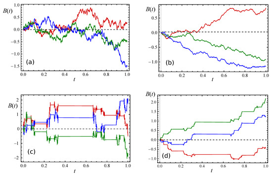
Figure 1. Trajectories of the stochastic processes under consideration. (a) The Brownian motion on a real line with $\gamma$-dimension = 1, $H=0.5$. (b) The fractional Brownian motion on a real line with $\gamma$-dimension = 1, $H=0.75$. (c) The Brownian motion on a Cantor-like set with $\gamma$-dimension = $\alpha =0.5$, $H=0.25$. (d) The fractional Brownian motion on a Cantor-like set with $\gamma$-dimension = $\alpha =0.5$, $H=0.375$.

5. Fractional Brownian Motion on Fractal Sets

In this section, we define the Fractional Brownian Motion (FBM) with fractal support in terms of probability density function, stochastic process, and fractal stochastic integral [36,37,40,41,42,43,44,45].

It is known that the FBM is a random walk with a continuous time parameter space, which provides useful models for many physical phenomena for which the empirical spectral power is given by a fractional law. FBM is defined by the so-called Hurst exponent $H\in (0,1)$. The increments of FBM are correlated (except the case $H=1/2$) and obtained from Gaussian noise via fractional integral [44],

$$B_H\left(t\right)=\frac{1}{\mathsf{\Gamma }(H+1/2)}{\int }_{-\infty }^{\infty }\left[{(t-t^{\prime })}_{+}^{H-1/2}-{(-t^{\prime })}_{+}^{H-1/2}\right]dB\left(t^{\prime }\right).$$

(41)

producing an auto-correlation function

$$⟨B_H\left(t_1\right)B_H\left(t_2\right)⟩=C\left[|t_1{|}^{2H}+|t_2{|}^{2H}-{|t_1-t_2|}^{2H}\right],$$

(42)

where C is a constant. Here, ${(t-t^{\prime })}_{+}=0$, if $(t-t^{\prime })<0$.

When $H=1/2$, FBM becomes the ordinary BM. If $1/2<H<1$, we have superdiffusion (enhanced diffusion), and if $H<1/2$, the process is subdiffusive. FBM is non-stationary and non-Markovian but with stationary-dependent increments with normal distribution. It has a self-similar structure, and it is defined as a stochastic integral of white noise. Its transition probability function is a normal distribution, which is the solution for heat equation. FBM is the generalization of the BM, which allows its increment to be correlated over time which can be positive/persistent correlation or negative/anti-persistent correlation. On one hand, the fractional Gaussian noise (FGN) is defined as the stochastic derivative of FBM. On the other hand, the stochastic integration of FGN gives FBM; therefore, both of them are characterized by Hurst parameter $(0<H<1)$, which is defined by $Q\propto {(\Delta t)}^H$, where Q is standard derivation and $\Delta t$ indicates lag time. FBMs are characterized by H in this way if $H<0.5$. it is called anti-persistent, persistent if $0.5<H$, and Brownian motion if $H=0.5$. FBM is called a non-stationary stochastic process with time-dependence variance, while FGN is stationary. Fractional derivatives (FDs) were used to define FBM and show its properties; hence, both of them are associated with anomalous diffusion. The fractional models have proven a linear relation with the order of derivatives and fractal dimensions. FBMs trajectories are continuous but non-differentiable in the sense of standard calculus. Anomalous diffusion in strong disorder media was studied by using FBM and the corresponding mean square passion that does not increase linearly with time. The DNA sequence was studied by using signal processing technique, which leads to FBM [36,37,38,39,40,41,42,43,44,45,48,49].

The mean square displacement of different random walks was explained using fractal derivatives [24,50]. Non-local derivatives were defined to model processes with long-memory properties on fractal sets [35]. Several phenomena involving fractal time are very interesting, and it is important to study them [51,52]. Equilibrium and non-equilibrium statistical mechanics involving generalized fractal derivatives were reviewed [53].

First representation: To model anomalous sub-diffusion using non-local derivatives, which is called fractal fractional Brownian motion, we have

$$\begin{array}{ccc}\hfill D_{F,t}^{\zeta }p(x,t)& =& {}_0{\mathcal{D}}_t^{1-\beta }\left({\mathsf{\Gamma }}_F^{\zeta }\left(\beta \right)\mathbf{D}\right){\left(D_{F,x}^{\alpha }\right)}^{2}p(x,t)\hfill \\ & =& {\left(S_F^{\zeta }\left(t\right)\right)}^{\beta -1}\mathbf{D}{\left(D_{F,x}^{\alpha }\right)}^2,\hfill \end{array}$$

(43)

where $\mathbf{D}$ is constant and $p(x,t)$ is the probability density function of fractal fractional Brownian motion. The solution of Equation (43) is

$$\begin{array}{ccc}\hfill p(x,t)& =& \frac{1}{\sqrt{4\pi D{\left(S_F^{\zeta }\left(t\right)\right)}^{\beta }}}exp\left[-\frac{S_F^{\alpha }{\left(x\right)}^2}{4\pi D{\left(S_F^{\zeta }\left(t\right)\right)}^{\beta }}\right].\hfill \end{array}$$

(44)

By using the upper bound of the staircase function,

$$0<S_F^{\zeta }\left(t\right)\le t^{\zeta },$$

(45)

Then, we have

$$\begin{array}{ccc}\hfill p(x,t)& \approx & \frac{1}{\sqrt{4\pi D{t}^{\zeta \beta }}}exp\left[-\frac{x^{2\alpha }}{4\pi D{t}^{\zeta \beta }}\right],0<\beta <\zeta ,\hfill \end{array}$$

(46)

where $\zeta$ and $\alpha$ are fractal dimensions of the time and space, respectively, and $\beta$ is a free parameter, which is called the non-local order derivatives on fractal time space [54,55]. Using Equation (46), the mean square displacement is obtained as follows:

$$\begin{array}{c}\hfill <S_F^{\alpha }{\left(x\right)}^2>2D{\left(S_F^{\zeta }\left(t\right)\right)}^{\beta }.\end{array}$$

(47)

Using Equation (45), we obtain

$$\begin{array}{ccc}\hfill <S_F^{\alpha }{\left(x\right)}^2>& \approx & 2D{t}^{\zeta \beta }.\hfill \end{array}$$

(48)

The mean square displacement in terms of Hurst parameter H is defined as

$$\begin{array}{ccc}\hfill <S_F^{\alpha }{\left(x\right)}^2>& =& 2D{S}_F^{\zeta }{\left(t\right)}^{2H}.\hfill \end{array}$$

(49)

Utilizing Equation (45), we have

$$\begin{array}{ccc}\hfill <S_F^{\alpha }{\left(x\right)}^2>& \approx & 2D{t}^{2\zeta H}.\hfill \end{array}$$

(50)

Hence, we get

$$\begin{array}{c}\hfill \beta =2H,\end{array}$$

(51)

and

$$\begin{array}{c}\hfill H_F^{\zeta }=\zeta H,\end{array}$$

(52)

where $H_F^{\zeta }$ is the fractal Hurst exponent. We note that the fractal power law diffusivity is related to fractional derivative.

Second representation: The fractional Brownian motion on thin Cantor-like sets is defined as a stochastic process with the following properties. Let $B^{H_F^{\zeta }}\left(t\right)=B_F^{\zeta }\left(t\right)$ and $H_F^{\zeta }\in [0,\zeta ]$, then its correlations function and self similarity properties can be expressed as follows:

(1) Correlations:

$$\begin{array}{cc}\hfill & E\left(B_F^{\zeta }\left(t\right)B_F^{\zeta }\left(s\right)\right)=\mathrm{Corr}(t,s)=\frac{1}{2}\left(|S_F^{\zeta }{\left(t\right)|}^{2H}+|S_F^{\zeta }{\left(s\right)|}^{2H}-{|S_F^{\zeta }\left(t\right)-S_F^{\zeta }\left(s\right)|}^{2H}\right),\hfill \end{array}$$

(53)

or its approximation

$$\mathrm{Corr}(t,s)\approx \frac{1}{2}\left(|t^{\zeta }{|}^{2H}+|s^{\zeta }{|}^{2H}-{|t^{\zeta }-s^{\zeta }|}^{2H}\right),t,s\in F.$$

(54)

(2) Self Similarity:

$$B_F^{\zeta }\left(at\right)\sim a^{H_F^{\zeta }}{B}_F^{\zeta }\left(t\right).$$

(55)

(3) Second moment:

$$\begin{array}{cc}\hfill & E{(B_F^{\zeta }\left(t\right)-B_F^{\zeta }\left(s\right))}^2=E{\left(B_F^{\zeta }\left(t\right)\right)}^2+E{\left(B_F^{\zeta }\left(s\right)\right)}^2-2E\left(B_F^{\zeta }\left(t\right)B_F^{\zeta }\left(s\right)\right)\hfill \\ & =|S_F^{\zeta }{\left(t\right)|}^{2H}+|S_F^{\zeta }{\left(s\right)|}^{2H}-|S_F^{\zeta }{\left(t\right)|}^{2H}-|S_F^{\zeta }{\left(s\right)|}^{2H}+{|S_F^{\zeta }\left(t\right)-S_F^{\zeta }\left(s\right)|}^{2H}\hfill \\ & =|S_F^{\zeta }\left(t\right)-S_F^{\zeta }{\left(s\right)|}^{2H}.\hfill \end{array}$$

(56)

Third representation: The fractal fractional Brownian motion is defined by [44]

$$\begin{array}{c}\hfill B^{H_F^{\zeta }}\left(t\right)=\frac{1}{{\mathsf{\Gamma }}_F^{\alpha }(H_F^{\zeta }+\frac{1}{2})}{\int }_0^t{(t-s)}^{(H_F^{\zeta }-1/2)}{d}_F^{\alpha }B\left(s\right),\end{array}$$

(57)

where we suppose

$$\varphi \left(s\right)={(t-s)}^{(H_F^{\zeta }-1/2)}.$$

(58)

To interpret Equations (57) and (58), we define them for the partition $t_1=a,...,t_l=b$ and $s\in (t_j,t_{j+1}],s\in F$ as follows:

$$\begin{array}{ccc}\hfill {\int }_a^b\varphi \left(s\right)d_F^{\alpha }B\left(s\right)& =& \sum _{n=1}^l\varphi \left(s\right)\mathsf{\Gamma }(\alpha +1){\left(B^{H_F^{\zeta }}\left(t_{j+1}\right)-B^{H_F^{\zeta }}\left(t_j\right)\right)}^{\alpha }\hfill \\ & =& \sum _{n=1}^l\varphi \left(j\right)\mathsf{\Gamma }(\alpha +1){\left(B^{H_F^{\zeta }}\left(t_{j+1}\right)-B^{H_F^{\zeta }}\left(t_j\right)\right)}^{\alpha }.\hfill \end{array}$$

(59)

In Figure 1, we sketched the fractional Brownian motion on a real line and on fractal sets.

6. Spectral Density of Fractional Brownian Motion on Fractal Sets

In this section, we analyze the spectral density FBM on fractal sets. Because of the conjugacy between the fractal calculus and standard calculus, we suggest the following spectral density:

$$p_{B_F^{\xi }}\left(\omega \right)=C_{-}^{\alpha }\underset{T\to \infty }{lim}{p}_{B_{F,T}^{\xi }}\left(\omega \right)=C_{-}^{\alpha }\underset{T\to \infty }{lim}\frac{1}{T}E{\left|\widehat{B}\left(\omega \right)\right|}^2,$$

(60)

where

$$\widehat{B}\left(\omega \right)={\int }_{t_0}^{t_0+T}{B}_F^{\zeta }\left(t\right)d_F^{\alpha }t,$$

(61)

is the fractal Fourier of $B_F^{\zeta }\left(t\right)$ and

$$\begin{array}{cc}\hfill & E|\widehat{B}{\left(\omega \right)|}^2\hfill \\ & ={\int }_{t_0}^{t_0+T}{\int }_{t_0}^{t_0+T}E\left(B_F^{\zeta }\left(t_1\right)B_F^{\zeta }\left(t_2\right)\right)e^{-i{S}_F^{\zeta }\left(\omega \right)(S_F^{\zeta }\left(t_1\right)-S_F^{\zeta }\left(t_2\right))}{d}_F^{\alpha }{t}_1{d}_F^{\alpha }{t}_2,\hfill \end{array}$$

(62)

where

$$\begin{array}{cc}\hfill & E\left(B_F^{\zeta }\left(t_1\right)B_F^{\zeta }\left(t_2\right)\right)\hfill \\ & =\frac{1}{2}\left(\right|S_F^{\zeta }\left(t_1\right)-S_F^{\zeta }\left(t_0\right){|}^{2H}+|S_F^{\zeta }\left(t_2\right)-S_F^{\zeta }\left(t_0\right){|}^{2H}-|S_F^{\zeta }\left(t_2\right)-S_F^{\zeta }\left(t_1\right){|}^{2H}).\hfill \end{array}$$

(63)

By virtue of the conjugacy of fractal calculus with the ordinary one, we can write the following:

$$\begin{array}{cc}\hfill p_{B_{F,T}^{\xi }}\left(\omega \right)& =\left\{\begin{array}{cc}\frac{S_F^{\zeta }{\left(T\right)}^{2H+1}}{2(H+1)},\hfill & S_F^{\zeta }\left(\omega \right)=0;\hfill \\ \frac{\pi }{4}(2H\frac{{\pi }^{2H-1}}{{\left(S_F^{\zeta }\left(\omega \right)\right)}^{2H+1}}+\frac{S_F^{\zeta }{\left(T\right)}^{2H-1}}{S_F^{\zeta }{\left(\omega \right)}^2}),\hfill & S_F^{\zeta }\left(\omega \right)\ne 0.\hfill \end{array}\right.\hfill \\ \hfill & \propto \left\{\begin{array}{cc}\frac{T^{\zeta (2H+1)}}{2(H+1)},\hfill & S_F^{\zeta }\left(\omega \right)=0;\hfill \\ \frac{\pi }{4}(2H\frac{{\pi }^{2H-1}}{{\left(\omega \right)}^{\zeta (2H+1)}}+\frac{T^{\zeta (2H-1)}}{{\left(\omega \right)}^{2\zeta }}),\hfill & S_F^{\zeta }\left(\omega \right)\ne 0.\hfill \end{array}\right.\hfill \end{array}$$

(64)

and

$$\begin{array}{cc}\hfill p_{B_F^{\xi }}\left(\omega \right)& =\left\{\begin{array}{cc}\infty ,\hfill & S_F^{\zeta }\left(\omega \right)=0,0<H<1,\hfill \\ \frac{H{\pi }^{2H}}{2}\frac{1}{S_F^{\zeta }{\left(\omega \right)}^{(2H+1)}},\hfill & S_F^{\zeta }\left(\omega \right)\ne 0,0<H<1/2,\hfill \\ \frac{\pi }{2}\frac{1}{S_F^{\zeta }{\left(\omega \right)}^2},\hfill & S_F^{\zeta }\left(\omega \right)\ne 0,H=1/2,\hfill \\ \infty ,\hfill & S_F^{\zeta }\left(\omega \right)\ne 0,1/2<H<1.\hfill \end{array}\right.\hfill \\ & \propto \{\begin{array}{cc}\infty ,\hfill & S_F^{\zeta }\left(\omega \right)=0,0<H<1,\hfill \\ \frac{H{\pi }^{2H}}{2}\frac{1}{{\omega }^{\zeta (2H+1)}},\hfill & S_F^{\zeta }\left(\omega \right)\ne 0,0<H<1/2,\hfill \\ \frac{\pi }{2}\frac{1}{{\omega }^{2\zeta }},\hfill & S_F^{\zeta }\left(\omega \right)\ne 0,H=1/2,\hfill \\ \infty ,\hfill & S_F^{\zeta }\left(\omega \right)\ne 0,1/2<H<1.\hfill \end{array}\hfill \end{array}$$

(65)

Remark 1.

For example, if we consider FBM on the triadic Cantor set ($\zeta =0.6$), then the Hurst parameter $0<H<0.6$; in particular, we can characterize it as follows: if $H<0.3$, then we have anti-persistent FBM, FBM persistent if $0.3<H$, and BM if $H=0.3$.

Using the virtue of spectral density, we can also categorize FBM on the triadic Cantor set as follows: if $0<H\le 0.3$, then by using Equation (65), we have $p_{B_F^{\xi }}\left(\omega \right)\propto {\omega }^{-0.6(2H+1)}$. In addition, from Equation (64), if $0<H\le 0.3\Rightarrow p_{B_F^{\xi },T}\left(\omega \right)\propto {\omega }^{-0.6(2H+1)}$, but $0.3<H<0.6\Rightarrow p_{B_F^{\xi },T}\left(\omega \right)\propto {\omega }^{-1.2}$.

Remark 2.

Throughout the paper, one can obtain the standard results by choosing $\alpha =1$ (see [42,43,44,45,56,57,58]).

7. Conclusions

In this paper, we considered fractal generalizations of Brownian motion and fractional Brownian motion. These generalized processes were defined with the use of fractal calculus. Fractalized fractional Brownian motion was given using non-local fractal derivatives, stochastic processes, and stochastic integrals on thin Cantor-like sets. The fractal Hurst exponent/parameter was defined as a characterized FFBM. The sample Brownian motion and FFBM were plotted to show the validity of our obtained results. We claim that fractal derivative defined on the one-sided Lévy–Lorentz set becomes fractional derivative after the averaging procedure over the ensemble of random realizations. The counting process defined on a corresponding fractal time set becomes the fractional Poisson process. In this case, the fractal derivative is the progenitor of the fractional derivative, which arises if we use a certain fractal distribution of events on the time axis.

References

- Mandelbrot, B.B. The Fractal Geometry of Nature; WH Freeman: New York, NY, USA, 1983; Volume 173. [Google Scholar]
- Mandelbrot, B.B. Fractals: Form, Chance and Dimension; WH Freeman Co.: San Francisco, CA, USA, 1979. [Google Scholar]
- Schroeder, M. Fractals, Chaos, Power Laws: Minutes from an Infinite Paradise; Courier Corporation: North Chelmsford, MA, USA, 2009. [Google Scholar]
- Graf, S.; Zähle, M. Fractal Geometry and Stochastics; Bandt, C., Ed.; Birkhäuser: Basel, Switzerland, 1995. [Google Scholar]
- Barnsley, M.F.; Devaney, R.L.; Mandelbrot, B.B.; Peitgen, H.O.; Saupe, D.; Voss, R.F. The Science of Fractal Images; Springer: New York, NY, USA, 1988. [Google Scholar]
- Nottale, L. Fractal Space-Time and Microphysics: Towards a Theory of Scale Relativity; World Scientific: Singapore, 1993. [Google Scholar]
- Parvate, A.; Gangal, A.D. Calculus on fractal subsets of real-line I: Formulation. Fractals 2009, 17, 53–148. [Google Scholar] [CrossRef]
- Parvate, A.; Gangal, A.D. Calculus on fractal subsets of real line II: Conjugacy with ordinary calculus. Fractals 2011, 19, 271–290. [Google Scholar] [CrossRef]
- Satin, S.; Parvate, A.; Gangal, A.D. Fokker-Planck equation on fractal curves. Chaos Solitons Fract. 2013, 52, 30–35. [Google Scholar] [CrossRef]
- Parvate, A.; Satin, S.; Gangal, A.D. Calculus on fractal curves in Rn. Fractals 2011, 19, 15–27. [Google Scholar] [CrossRef]
- Satin, S.; Gangal, A.D. Langevin Equation on Fractal Curves. Fractals 2016, 24, 1650028. [Google Scholar] [CrossRef]
- Nigmatullin, R.R. The realization of the generalized transfer equation in a medium with fractal geometry. Phys. Status Solidi B 1986, 133, 425–430. [Google Scholar] [CrossRef]
- Rutman, R.S. On the paper by RR Nigmatullin “Fractional integral and its physical interpretation”. Theor. Math. Phys. 1994, 100, 1154–1156. [Google Scholar] [CrossRef]
- Hilfer, R.; Anton, L. Fractional master equations and fractal time random walks. Phys. Rev. E. 1995, 51, R848. [Google Scholar] [CrossRef] [PubMed]
- Sibatov, R.T.; Sun, H. Tempered fractional equations for quantum transport in mesoscopic one-dimensional systems with fractal disorder. Fractal Fract. 2019, 3, 47. [Google Scholar] [CrossRef]
- Rocco, A.; West, B.J. Fractional calculus and the evolution of fractal phenomena. Physica A 1999, 265, 535–546. [Google Scholar] [CrossRef]
- Metzler, R.; Klafter, J.; Sokolov, I.M. Anomalous transport in external fields: Continuous time random walks and fractional diffusion equations extended. Phys. Rev. E 1998, 58, 1621. [Google Scholar] [CrossRef]
- Barkai, E. Fractional Fokker-Planck equation, solution, and application. Phys. Rev. E 2001, 63, 046118. [Google Scholar] [CrossRef]
- Laskin, N. Fractional poisson process. Comm. Nonlinear Sci. Numer. Simulat. 2003, 8, 201–213. [Google Scholar] [CrossRef]
- Golmankhaneh, A.K.; Tunc, C. Stochastic differential equations on fractal sets. Stochastics 2019, 92, 1–17. [Google Scholar] [CrossRef]
- Golmankhaneh, A.K.; Cattani, C. Fractal Logistic Equation. Fractal Fract. 2019, 3, 41. [Google Scholar] [CrossRef]
- Golmankhaneh, A.K.; Fernandez, A. Random Variables and Stable Distributions on Fractal Cantor Sets. Fractal Fract. 2019, 3, 31. [Google Scholar] [CrossRef]
- El-Nabulsi, R.A.; Golmankhaneh, A.K. On fractional and fractal Einstein’s field equations. Mod. Phys. Lett. 2021. [Google Scholar] [CrossRef]
- Golmankhaneh, A.K.; Balankin, A.S. Sub-and super-diffusion on Cantor sets: Beyond the paradox. Phys. Lett. A 2018, 382, 960–967. [Google Scholar] [CrossRef]
- Golmankhaneh, A.K.; Ali, K.K. Fractal Kronig-Penney model involving fractal comb potential. J. Math. Model. 2021. [Google Scholar] [CrossRef]
- Barkai, E.; Fleurov, V.; Klafter, J. One-dimensional stochastic Lévy-Lorentz gas. Phys. Rev. E 2000, 61, 1164. [Google Scholar] [CrossRef]
- Nigmatullin, R.R.; Zhang, W.; Gubaidullin, I. Accurate relationships between fractals and fractional integrals: New approaches and evaluations. Fract. Calc. Appl. Anal. 2017, 20, 1263–1280. [Google Scholar] [CrossRef]
- Uchaikin, V.V. Self-similar anomalous diffusion and Lévy-stable laws. Physics-Uspekhi 2003, 46, 821. [Google Scholar] [CrossRef]
- Uchaikin, V.V.; Cahoy, D.O.; Sibatov, R.T. Fractional processes: From Poisson to branching one. Int. J. Bifurcat. Chaos 2008, 18, 2717–2725. [Google Scholar] [CrossRef]
- Uchaikin, V.V.; Sibatov, R.T. Fractional Kinetics in Solids: Anomalous Charge Transport in Semiconductors, Dielectrics, and Nanosystems; World Scientific: Singapore, 2013. [Google Scholar]
- Hilfer, R. Exact solutions for a class of fractal time random walks. Fractals 1995, 3, 211–216. [Google Scholar] [CrossRef]
- Zhokh, A.; Trypolskyi, A.; Strizhak, P. Relationship between the anomalous diffusion and the fractal dimension of the environment. Chem. Phys. 2018, 503, 71–76. [Google Scholar] [CrossRef]
- Zhokh, A.; Strizhak, P. Non-Fickian transport in porous media: Always temporally anomalous? Transp. Porous Media 2018, 124, 309–323. [Google Scholar] [CrossRef]
- Papoulis, A.; Pillai, S.U. Probability, Random Variables, and Stochastic Processes, 4th ed.; McGraw-Hill: New York, NY, USA, 2002. [Google Scholar]
- Golmankhaneh, A.K.; Baleanu, D. Non-local Integrals and Derivatives on Fractal Sets with Applications. Open Phys. 2016, 14, 542–548. [Google Scholar] [CrossRef]
- Duncan, T.E. Some aspects of fractional Brownian motion. Nonlinear Anal. Theory Methods Appl. 2001, 47, 4775–4782. [Google Scholar] [CrossRef]
- Chow, W.C. Fractal (fractional) Brownian motion, Wiley Interdiscip. Rev. Comput. Stat. 2011, 3, 149–162. [Google Scholar]
- Butera, S.; Paola, M.D. A physically based connection between fractional calculus and fractal geometry. Ann. Phys. 2014, 350, 146–158. [Google Scholar] [CrossRef]
- Tatom, F.B. The relationship between fractional calculus and fractals. Fractals 1995, 3, 217–229. [Google Scholar] [CrossRef]
- Machado, J.A.T. Fractional order description of DNA. Appl. Math. Model. 2015, 39, 4095–4102. [Google Scholar] [CrossRef]
- Zunino, L.; Pérez, D.G.; Kowalski, A.; Martín, M.T.; Garavaglia, M.; Plastino, A.; Rosso, O.A. Fractional Brownian motion, fractional Gaussian noise, and Tsallis permutation entropy. Physica A 2008, 387, 6057–6068. [Google Scholar] [CrossRef]
- Shevchenko, G. Fractional Brownian motion in a nutshell. arXiv 2014, arXiv:1406.1956. [Google Scholar] [CrossRef]
- Ortigueira, M.D.; Batista, A.G. A fractional linear system view of the fractional brownian motion. Nonlinear Dyn. 2004, 38, 295–303. [Google Scholar] [CrossRef][Green Version]
- Mandelbrot, B.B.; Van Ness, J.W. Fractional Brownian motions, fractional noises and applications. SIAM Rev. 1968, 10, 422–437. [Google Scholar] [CrossRef]
- Nourdin, I. Selected Aspects of Fractional Brownian Motion; Springer: Milan, Italy, 2012; Volume 4. [Google Scholar]
- Prodanov, D. Characterization of the local growth of two Cantor-type functions. Fractal Fract. 2019, 3, 45. [Google Scholar] [CrossRef]
- Wibowo, S.; Kurniawan, V.Y. The relation between Hölder continuous function of order α∈(0,1) and function of bounded variation. J. Phys. Conf. Ser. 2020, 1490, 012043. [Google Scholar] [CrossRef]
- Dos Santos, M.A.F. A fractional diffusion equation with sink term. Indian J. Phys. 2020, 94, 1123–1133. [Google Scholar] [CrossRef]
- Dos Santos, M.A.F. Analytic approaches of the anomalous diffusion: A review. Chaos Solitons Fractals 2019, 124, 86–96. [Google Scholar] [CrossRef]
- Sandev, T.; Iomin, A.; Kantz, H. Anomalous diffusion on a fractal mesh. Phys. Rev. E 2017, 95, 052107. [Google Scholar] [CrossRef]
- Welch, K. A Fractal Topology of Time: Deepening into Timelessness, 2nd ed.; Fox Finding Press: Austin, TX, USA, 2020. [Google Scholar]
- Shlesinger, M.F. Fractal time in condensed mattar. Ann. Rev. Phys. Chern. 1988, 39, 269–290. [Google Scholar] [CrossRef]
- Golmankhaneh, A.K.; Welch, K. Equilibrium and non-equilibrium statistical mechanics with generalized fractal derivatives: A review. Mod. Phys. Lett. 2021. [Google Scholar] [CrossRef]
- Bodrova, A.S.; Chechkin, A.V.; Cherstvy, A.G.; Safdari, H.; Sokolov, I.M.; Metzler, R. Underdamped scaled Brownian motion: (Non-)existence of the overdamped limit in anomalous diffusion. Sci. Rep. 2016, 6, 30520. [Google Scholar] [CrossRef]
- Golmankhaneh, A.K. On the fractal Langevin equation. Fractal Fract. 2019, 3, 11. [Google Scholar] [CrossRef]
- Kuleshov, E.L.; Grudin, B.N. Spectral density of a fractional Brownian process. Optoelectron. Instrument. Proc. 2013, 49, 228–233. [Google Scholar] [CrossRef]
- Øigård, T.A.; Hanssen, A.; Scharf, L.L. Spectral correlations of fractional Brownian motion. Phys. Rev. E 2006, 74, 031114. [Google Scholar] [CrossRef] [PubMed]
- Flandrin, P. On the spectrum of fractional Brownian motions. IEEE Trans. Inf. Theory 1989, 35, 197–199. [Google Scholar] [CrossRef]
Publisher’s Note: MDPI stays neutral with regard to jurisdictional claims in published maps and institutional affiliations. |
© 2021 by the authors. Licensee MDPI, Basel, Switzerland. This article is an open access article distributed under the terms and conditions of the Creative Commons Attribution (CC BY) license (http://creativecommons.org/licenses/by/4.0/).