Four-Quadrant Riemann Problem for a 2×2 System II

Abstract

In previous work, we considered a four-quadrant Riemann problem for a $2\times 2$ hyperbolic system in which delta shock appears at the initial discontinuity without assuming that each jump of the initial data projects exactly one plane elementary wave. In this paper, we consider the case that does not involve a delta shock at the initial discontinuity. We classified 18 topologically distinct solutions and constructed analytic and numerical solutions for each case. The constructed analytic solutions show the rich structure of wave interactions in the Riemann problem, which coincide with the computed numerical solutions.

1. Introduction

The two-dimensional scalar conservation law is given by

$$u_t+f{\left(u\right)}_x+g{\left(u\right)}_y=0,$$

(1)

where $u(x,y,t)$ is a conserved quantity, and f and g are nonlinear fluxes. Even though the existence and uniqueness theory for scalar hyperbolic equations in multiple dimensions is complete [1,2,3,4], it provides little insight into the qualitative behavior of wave interactions.

In 1975, Guckenheimer [5] initiated the construction of a solution for the two-dimensional (2-D) Riemann problem (RP) by developing an interesting example called the Guckenheimer structure. In 1983, Wagner [6] constructed a solution for the four-quadrant RP of a 2-D scalar conservation law with convex $f=g$. Lindquist showed that the Riemann solutions are piecewise smooth when $f=g$ [7] and outlined the construction method [8].

In contrast, because general theory does not exist for multidimensional systems, 2-D RP for systems must be investigated on a case-by-case basis. Glimm et al. [9] provided a list of generic waves expected in the 2-D RP solutions to the Euler equations. In 1990, Zhang and Zheng [10] proposed the structure for a solution to a four-quadrant RP for a 2-D gas dynamics system:

$$\left\{\begin{array}{c}{\rho }_t+{\left(\rho u\right)}_x+{\left(\rho v\right)}_y=0,\hfill \\ {\left(\rho u\right)}_t+{(\rho u^2+p)}_x+{\left(\rho uv\right)}_y=0,\hfill \\ {\left(\rho v\right)}_t+{\left(\rho uv\right)}_x+{(\rho v^2+p)}_y=0.\hfill \end{array}\right.$$

(2)

To prove this conjecture, many studies have been conducted on simplified gas-dynamics-like models, including pressure gradient, transportation, and Chaplygin gas dynamics models [11,12,13,14,15,16,17,18,19,20,21]. A good summary is provided in [22,23,24].

Most of the aforementioned RPs were conducted under the assumption [25]:

$$\begin{array}{cc}\left(H\right)\hfill & \mathit{Outside}\mathit{a}\mathit{neighborhood}\mathit{of}\mathit{the}\mathit{origin},\mathit{each}\mathit{jump}\mathit{of}\mathit{the}\mathit{initial}\mathit{data}\mathit{projects}\hfill \\ & \mathit{exactly}\mathit{one}\mathit{plane}\mathit{elementary}\mathit{wave}.\hfill \end{array}$$

Since 2002, only a few studies [26,27,28,29,30] have been conducted without assumption $\left(H\right)$. Hwang and Lindquist [26,27] initiated the removal of assumption $\left(H\right)$ in the 2-D RP for the generalized model of the 1-D Keyfitz–Kranzer–Isaacson-Temple model [31,32,33].

Shen et al. [28] classified and constructed ten solutions for the system (3) without $\left(H\right)$ using the transformation $\tilde{\xi }=(x+y)/2$ and $\tilde{\eta }=(y-x)/2$ because it is an isotropic model.

$$\left\{\begin{array}{c}{u}_t+{\left(u^2\right)}_x+{\left(u^2\right)}_y=0,\hfill \\ {\rho }_t+{\left(\rho u\right)}_x+{\left(\rho u\right)}_y=0.\hfill \end{array}\right.$$

(3)

Hwang et al. [30] classified and constructed 12 solutions for the system (3) in three constant states. In [34], a four-quadrant RP in which a delta shock appears at the initial discontinuity was considered. In this study, without assuming $\left(H\right)$, we consider a four-quadrant RP for the hyperbolic system (3) with initial data that do not involve a delta shock. Four-quadrant RPs for system (3) are formally classified into $5!=120$ cases. The cases including a delta shock were reduced to 52 cases, which resulted in 14 topologically distinct solutions [34]. By contrast, the cases that did not include a delta shock were reduced to 68 cases. In this study, we classified and constructed 18 topologically distinct solutions.

In Section 2, the construction method is described. Analytic and numerical solutions are presented in Section 3, and the discussion follows in Section 4. We present the conclusion in Section 5.

2. Construction Method

From the initial discontinuity between the two sides $(u_l,{\rho }_l)$ and $(u_r,{\rho }_r)$ in the counterclockwise direction, we use the notation $R_{lr},J_{lr},S_{lr}$ for the rarefaction wave, contact discontinuity, and shock, respectively.

The rarefaction wave $R_{lr}\left(\eta \right)$, contact discontinuity $J_{lr}\left(\eta \right)$, and shock $S_{lr}\left(\eta \right)$ that are parallel to the $\xi$-axis can be expressed as

$$R_{lr}\left(\eta \right):\eta =2u,\frac{\rho }{u}=\frac{{\rho }_l}{u_l},\left(u_r\le u\le u_l\mathrm{for}\eta >\xi ,u_l\le u\le u_r\mathrm{for}\eta <\xi \right).$$

(4)

$$J_{lr}\left(\eta \right):\eta =u_l=u_r,$$

(5)

$$\begin{array}{c}{S}_{lr}\left(\eta \right):\eta =u_l+u_r,\frac{{\rho }_r}{u_r}=\frac{{\rho }_l}{u_l},\\ \left(0<u_l<u_r\mathrm{or}{u}_l<u_r<0\mathrm{for}\eta >\xi ,0<u_r<u_l\mathrm{or}{u}_r<u_l<0\mathrm{for}\eta <\xi \right),\end{array}$$

(6)

respectively. The waves parallel to the $\eta$-axis can be described in a similar manner. The rarefaction $R_{lr}$, contact $J_{lr}$, and shock $S_{lr}$ are directed to singular points $(2u,2u),(u,u)$, and $(u_l+u_r,u_l+u_r)$, respectively.

We consider a four-quadrant RP for the system (3) in which the initial data do not involve a delta shock. We remove the assumption $\left(H\right)$; hence, there are one or two waves at infinity for each discontinuity.

Figure 1 shows wave curves in the phase plane for $u_2<u_3<u_4<0<u_1$. In the figure, from $(u_1,{\rho }_1)$ to $(u_2,{\rho }_2)$ we have one wave: a rarefaction wave $R_{12}$. From $(u_2,{\rho }_2)$ to the intermediate state $(u_b,{\rho }_b)$, there is a contact $J_{2b}$, and we have a shock $S_{b3}$ from $(u_b,{\rho }_b)$ to $(u_3,{\rho }_3)$. From $(u_3,{\rho }_3)$ to the intermediate state $(u_c,{\rho }_c)$, there is a rarefaction $R_{3c}$, and we have a contact $J_{c4}$ from $(u_c,{\rho }_c)$ to $(u_4,{\rho }_4)$. Finally, from $(u_4,{\rho }_4)$ to $(u_1,{\rho }_1)$, we have one wave which is a rarefaction $R_{41}$. Using the wave curves in the phase plane in Figure 1, we can locate the solution at infinity for each initial discontinuity in Figure 2. All the planar waves are parallel to each axes of initial discontinuity, and they are directed to their respective singular points. A new state $(u_b,{\rho }_b)$ is developed between $J_{2b}$ and $S_{b3}$, and the state $(u_b,{\rho }_b)$ is determined. The state $(u_b,{\rho }_b)$ satisfies $u_b=u_2$ and $\frac{{\rho }_b}{u_b}=\frac{{\rho }_3}{u_3}$. A new state $(u_c,{\rho }_c)$ is developed between $R_{3c}$ and $J_{c4}$, and the state $(u_c,{\rho }_c)$ is again determined. The state $(u_c,{\rho }_c)$ satisfies $u_c=u_4$ and $\frac{{\rho }_c}{u_c}=\frac{{\rho }_3}{u_3}$. The wave interactions in center region D in Figure 2 are then determined.

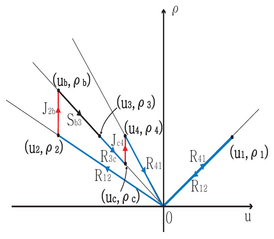
Figure 1. Wave curves in phase plane for $u_2<u_3<u_4<0<u_1$.

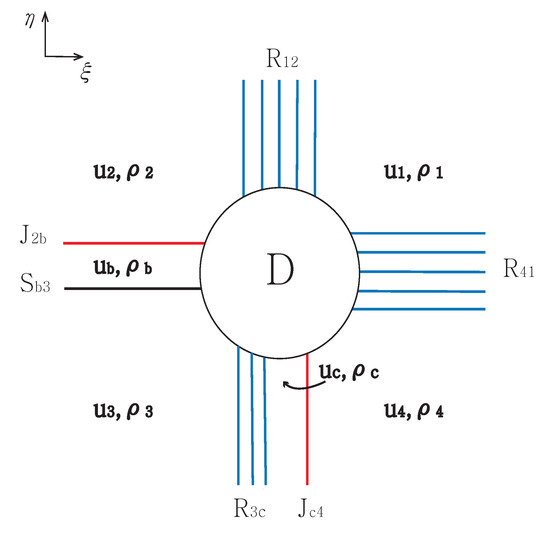
Figure 2. The solution at infinity $(R+JS+RJ+R)$ for $u_2<u_3<u_4<0<u_1$.

For the numerical solution, we modify the semi-discrete central upwind scheme by changing the flux functions to reduce the numerical dissipation of the contact discontinuity. Further details can be found in [30,35,36]. In this study, the computational domain is $[-4,4]\times [-4,4]$ and t = 0.2. ${\rho }_i=0.77$ for $i=1,\cdots ,4$. We used 1200 × 1200 cells, and the CFL was 0.05. We construct the solution on a case-by-case basis.

3. Construction of the Solution

For the classification of waves at the initial discontinuities, we count the exterior waves that come from the positive $\eta$-axis before those at the axes in the counterclockwise direction. In the classification of initial data, 03241 and 30412 indicate that $0<u_3<u_2<u_4<u_1$ and $u_3<0<u_4<u_1<u_2$, respectively.

3.1. No Shock

$$\begin{array}{c}Case1:RJ+RJ+JR+JR(03241,03421),JR+JR+RJ+RJ(32410,34210)\hfill \\ Case2:R+JR+R+JR\left(32041\right),RJ+R+RJ+R\left(34021\right)\hfill \\ Case3:R+JR+RJ+R(32401,34201),RJ+R+R+JR(30241,30421)\hfill \end{array}$$

Case 1.

$JR+JR+RJ+RJ(u_3<u_4<u_2<u_1<0)$

From the initial discontinuity, contact rarefaction is formed at each discontinuity. New states $(u_a,{\rho }_a),(u_b,{\rho }_b),(u_c,{\rho }_c)$ and $(u_d,{\rho }_d)$ satisfy $u_a=u_1,\frac{{\rho }_a}{u_a}=\frac{{\rho }_2}{u_2},u_b=u_2,\frac{{\rho }_b}{u_b}=\frac{{\rho }_3}{u_3},u_c=u_4,\frac{{\rho }_c}{u_c}=\frac{{\rho }_3}{u_3},$ and $u_d=u_1,\frac{{\rho }_d}{u_d}=\frac{{\rho }_4}{u_4}$, respectively. The contact discontinuities $J_{1a},J_{2b},J_{c4},$ and $J_{d1}$ are directed to the singular points $(u_1,u_1),(u_2,u_2),(u_4,u_4),$ and $(u_1,u_1)$, respectively.

The rarefactions $R_{a2},R_{b3},R_{3c},$ and $R_{4d}$ are directed to the singular points $(2u,2u)$ for $u_2\le u\le u_1,u_3\le u\le u_2,u_3\le u\le u_4,$ and $u_4\le u\le u_1$, respectively.

$J_{2b}$ completely penetrates $R_{a2}$ at point $A(2u_2,u_2)$, and the curved contact discontinuity $\eta =\eta \left(\xi \right)$ from A to $B(2u_1,\frac{2u_1{u}_2-u_1^2}{u_2})$ satisfies

$$\frac{d\eta }{d\xi }=\frac{\eta -u}{\xi -u},\xi =2u,\frac{\rho }{u}=\frac{{\rho }_2}{u_2},u_2\le u\le u_1,$$

(7)

which gives,

$$\eta =\xi +\frac{{\xi }^2}{4u_2},2u_2\le \xi \le 2u_1.$$

(8)

The straight contact discontinuity continues from point B to $C(u_1,u_1)$; it has the form:

$$\eta -u_1=\frac{u_2-u_1}{u_2}(\xi -u_1),2u_1\le \xi \le u_1.$$

(9)

The rarefaction waves $R_{b3}$ and $R_{3c}$, $R_{b3}$ and $R_{4d}$, $R_{a2}$ and $R_{4d}$ meet at the same singular point $(2u,2u)$ between $D(2u_3,2u_3)$ and $E(2u_4,2u_4)$, E and $F(2u_2,2u_2)$, F and $G(2u_1,2u_1)$, respectively. By contrast, $J_{c4}$ completely penetrates the rarefaction wave $R_{4d}$ at point $H(u_4,2u_4)$; then, the curved contact discontinuity satisfies

$$\frac{d\eta }{d\xi }=\frac{\eta -u}{\xi -u},\eta =2u,\frac{\rho }{u}=\frac{{\rho }_4}{u_4},u_4\le u\le u_1,$$

(10)

which gives

$$\xi =\eta +\frac{{\eta }^2}{4u_4},2u_4\le \eta \le 2u_1.$$

(11)

The straight contact discontinuity continues to the point $C(u_1,u_1)$, and it satisfies:

$$\eta -u_1=\frac{u_4}{u_4-u_1}(\xi -u_1),2u_1\le \eta \le u_1.$$

(12)

Thus, the four contact discontinuities meet at the singular point C. The solutions are shown in Figure 3. The initial conditions for the numerical computation are $u_1=-0.15,$$u_2=-0.37,$$u_3=-0.56,u_4=-0.43.$

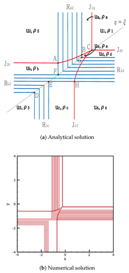
Figure 3. Case 1. JR + JR + RJ + RJ.

Case 2.

$R+JR+R+JR(u_3<u_2<0<u_4<u_1)$

From the initial discontinuity, a rarefaction is formed at the positive $\eta$-axis and negative $\eta$-axis, and contact rarefaction is formed at the negative $\xi$-axis and positive $\xi$-axis. The new states $(u_b,{\rho }_b)$ and $(u_d,{\rho }_d)$ satisfy $u_b=u_2,\frac{{\rho }_b}{u_b}=\frac{{\rho }_3}{u_3},$ and $u_d=u_4,\frac{{\rho }_d}{u_d}=\frac{{\rho }_1}{u_1}$, respectively. The rarefactions $R_{12},R_{b3},R_{34},$ and $R_{d1}$ are directed to the singular points $(2u,2u)$ for $u_2\le u\le u_1,u_3\le u\le u_2,u_3\le u\le u_4,$ and $u_4\le u\le u_1$, respectively. The contact discontinuities $J_{2b}$ and $J_{4d}$ are directed to the singular points $(u_2,u_2)$ and $(u_4,u_4)$, respectively.

The contact discontinuity $J_{2b}$ meets the rarefaction wave $R_{12}$ at point $A(2u_2,u_2)$; then the curved contact continues to point $O(0,0)$. The rarefaction waves $R_{b3}$ and $R_{34}$, $R_{12}$ and $R_{34}$, $R_{12}$ and $R_{d1}$ meet at $(2u,2u)$ between $B(2u_3,2u_3)$ and $C(2u_2,2u_2)$, C and $D(2u_4,2u_4)$, D and $E(2u_1,2u_1)$, respectively. By contrast, $J_{4d}$ meets the rarefaction wave $R_{34}$ at point $F(2u_4,u_4)$; then, the curved contact discontinuity continues to point O. The solutions are shown in Figure 4. The initial condition is $u_1=0.56,u_2=-0.29,u_3=-0.37,u_4=0.43.$

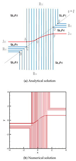
Figure 4. Case 2. R + JR + R + JR.

Case 3.

$RJ+R+R+JR(u_3<0<u_2<u_4<u_1)$

From the initial discontinuity, contact rarefaction is formed at the positive $\eta$-axis and positive $\xi$-axis, and the rarefaction wave is formed at the negative $\xi$-axis and negative $\eta$-axis. The contact discontinuity $J_{a2}$ meets the rarefaction wave $R_{23}$ at point $A(u_2,2u_2)$, and the curved contact then continues to point $O(0,0)$. The rarefaction waves $R_{23}$ and $R_{34}$, $R_{1a}$ and $R_{34}$, $R_{1a}$ and $R_{d1}$ meet at $(2u,2u)$ between $B(2u_3,2u_3)$ and $C(2u_2,2u_2)$, C and $D(2u_4,2u_4)$, D and $E(2u_1,2u_1)$, respectively. By contrast, $J_{4d}$ meets the rarefaction wave $R_{34}$ at point $F(2u_4,u_4)$; then the curved contact discontinuity continues to point O. The solutions are shown in Figure 5. The initial condition is $u_1=0.56,u_2=0.37,u_3=-0.15,u_4=0.43.$

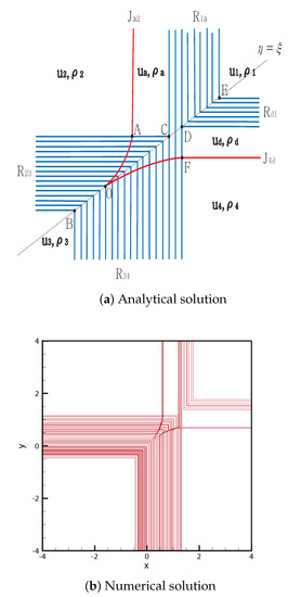
Figure 5. Case 3. RJ + R + R + JR.

3.2. One Shock

$$\begin{array}{c}Case4:\left\{\begin{array}{c}RJ+SJ+JR+JR\left(02341\right),RJ+RJ+JS+JR\left(04321\right)\hfill \\ JR+JR+RJ+SJ\left(32140\right),JS+JR+RJ+RJ\left(34120\right)\hfill \end{array}\right.\hfill \\ Case5:\left\{\begin{array}{c}RJ+RJ+JR+JS\left(03214\right),SJ+RJ+JR+JR\left(03412\right)\hfill \\ JR+JS+RJ+RJ\left(23410\right),JR+JR+SJ+RJ\left(43210\right)\hfill \end{array}\right.\hfill \\ Case6:\left\{\begin{array}{c}R+JS+R+JR\left(23041\right),R+JR+R+JS\left(32014\right)\hfill \\ SJ+R+RJ+R\left(34012\right),RJ+R+SJ+R\left(43021\right)\hfill \end{array}\right.\hfill \\ Case7:\left\{\begin{array}{c}R+JS+RJ+R\left(23401\right),R+JR+SJ+R\left(43201\right)\hfill \\ RJ+R+R+JS\left(30214\right),SJ+R+R+JR\left(30412\right)\hfill \end{array}\right.\hfill \end{array}$$

Case 4.

$JR+JR+RJ+SJ(u_3<u_2<u_1<u_4<0)$

From the initial discontinuity, contact shock is formed at the positive $\xi$-axis, and contact rarefaction is formed at the remaining three axes. The contact discontinuity $J_{2b}$ completely penetrates the rarefaction wave $R_{a2}$, and the straight contact discontinuity $J_{ae}$ continues from $A(2u_1,\frac{2u_1{u}_2-u_1^2}{u_2})$ to $B(u_1,u_1)$. The rarefaction waves $R_{b3}$ and $R_{3c}$, $R_{a2}$ and $R_{3c}$ meet at $(2u,2u)$ between $C(2u_3,2u_3)$ and $D(2u_2,2u_2)$, D and $E(2u_1,2u_1)$, respectively.

By contrast, $J_{c4}$ intersects with shock $S_{4d}$ at point $F(u_4,u_4+u_1)$, and the new contact discontinuity $J_{ed}$ from F to B satisfies:

$$\eta -u_1=\frac{u_4}{u_4-u_1}(\xi -u_1),u_1\le \xi \le u_4.$$

(13)

Thus, four contact discontinuities $J_{1a},J_{ae},J_{ed}$, and $J_{d1}$ meet at the singular point B.

The shock $S_{ce}(=S_{4d})$ satisfies the rarefaction wave $R_{3c}$ at point $G(2u_4,u_4+u_1)$; the curved shock then continues to point E. The curved shock from G to E satisfies:

$$\frac{d\eta }{d\xi }=\frac{\eta -(u+u_e)}{\xi -(u+u_e)},\xi =2u,\frac{\rho }{u}=\frac{{\rho }_3}{u_3},u_2\le u\le u_4,$$

(14)

and we obtain

$$\eta =\xi +\frac{1}{u_e-u_c}{\left(\frac{\xi }{2}-u_e\right)}^2,2u_2\le \xi \le 2u_4.$$

(15)

The solutions are shown in Figure 6. The initial condition is $u_1=-0.37,u_2=-0.43,$$u_3=-0.56,u_4=-0.15.$

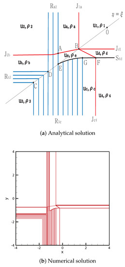
Figure 6. Case 4. JR + JR + RJ + SJ.

Case 5.

$SJ+RJ+JR+JR(0<u_3<u_4<u_1<u_2)$

From the initial discontinuity, contact shock is formed at the positive $\eta$-axis, and contact rarefaction is formed at the remaining three axes. $J_{a2}$ penetrates the entire rarefaction wave $R_{2b}$ and stops at the singular point $A(u_3,u_3)$. The shock $S_{1a}$ meets $R_{2b}$ at point $B(u_1+u_2,2u_2)$, and the curved shock then continues to point $C(2u_1,2u_1)$. The rarefaction waves $R_{2b}$ and $R_{c4}$, $R_{2b}$ and $R_{d1}$ meet at $(2u,2u)$ between $D(2u_3,2u_3)$ and $E(2u_4,2u_4)$, E and C, respectively. By contrast, the contact discontinuity $J_{4d}$ completely penetrates $R_{c4}$ and stops at the singular point A. Therefore, four contact discontinuities $J_{eb},J_{b3},J_{3c}$, and $J_{ce}$ meet at the singular point A. The solutions are shown in Figure 7. The initial condition is $u_1=0.43,u_2=0.56,u_3=0.15,u_4=0.37.$

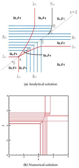
Figure 7. Case 5. SJ + RJ + JR + JR.

Case 6.

$SJ+R+RJ+R(u_3<u_4<0<u_1<u_2)$

From the initial discontinuity, rarefaction is formed at the negative $\xi$-axis and positive $\xi$-axis, and contact shock and contact rarefaction are formed at the positive $\eta$-axis and negative $\eta$-axis, respectively. The contact discontinuity $J_{a2}$ meets the rarefaction wave $R_{23}$ at point $A(u_2,2u_2)$, and the curved contact discontinuity then continues to point $O(0,0)$. $S_{1a}$ meets $R_{23}$ at point $B(u_1+u_2,2u_2)$. The curved shock then continues to point $C(2u_1,2u_1)$. The rarefaction waves $R_{23}$ and $R_{3c}$, $R_{23}$ and $R_{41}$ meet at $(2u,2u)$ between $D(2u_3,2u_3)$ and $E(2u_4,2u_4)$, E and C, respectively. By contrast, $J_{c4}$ meets the rarefaction wave $R_{41}$ at point $F(u_4,2u_4)$, and the curved contact discontinuity then continues to point O. The solutions are shown in Figure 8. The initial condition is $u_1=0.43,u_2=0.56,u_3=-0.37,u_4=-0.15.$

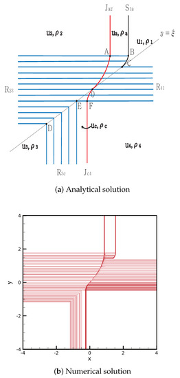
Figure 8. Case 6. SJ + R + RJ + R.

Case 7.

$R+JS+RJ+R(u_2<u_3<u_4<0<u_1)$

From the initial discontinuity, rarefaction is formed at the positive $\eta$-axis and positive $\xi$-axis, and contact shock and contact rarefaction are formed at the negative $\xi$-axis and negative $\eta$-axis, respectively. The contact discontinuity $J_{2b}$ meets the rarefaction wave $R_{12}$ at point $A(2u_2,u_2)$, and the curved contact then continues to point $O(0,0)$. $S_{b3}$ meets $R_{12}$ at point $B(2u_2,u_2+u_3)$, and the curved shock then continues to point $C(2u_3,2u_3)$. Rarefaction waves $R_{12}$ and $R_{3c}$, $R_{12}$ and $R_{41}$ meet at $(2u,2u)$ between C and $D(2u_4,2u_4)$, D and $E(2u_1,2u_1)$, respectively. By contrast, $J_{c4}$ meets the rarefaction wave $R_{41}$ at point $F(u_4,2u_4)$, and the curved contact discontinuity continues to point O. The solutions are shown in Figure 9. The initial condition is $u_1=0.15,u_2=-0.56,u_3=-0.43,u_4=-0.37.$

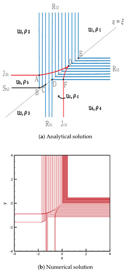
Figure 9. Case 7. R + JS + RJ + R.

3.3. Two Shocks

$$\begin{array}{c}Case8:SJ+RJ+JR+JS(01324,01342),JR+JS+SJ+RJ(24130,42130)\hfill \\ Case9:\left\{\begin{array}{c}RJ+SJ+JR+JS\left(02134\right),SJ+RJ+JS+JR\left(04132\right)\hfill \\ JR+JS+RJ+SJ\left(21340\right),JS+JR+SJ+RJ\left(41320\right)\hfill \end{array}\right.\hfill \\ Case10:\left\{\begin{array}{c}RJ+SJ+JR+JS\left(02314\right),SJ+RJ+JS+JR\left(04312\right)\hfill \\ JR+JS+RJ+SJ\left(23140\right),JS+JR+SJ+RJ\left(43120\right)\hfill \end{array}\right.\hfill \\ Case11:RJ+SJ+JS+JR(02413,04213),JS+JR+RJ+SJ(13240,13420)\hfill \\ Case12:RJ+SJ+JS+JR(02431,04231),JS+JR+RJ+SJ(31240,31420)\hfill \\ Case13:SJ+RJ+JR+JS(03124,03142),JR+JS+SJ+RJ(24310,42310)\hfill \\ Case14:R+JS+R+JS\left(23014\right),SJ+R+SJ+R\left(43012\right)\hfill \\ Case15:R+JS+SJ+R(24301,42301),SJ+R+R+JS(30124,30142)\hfill \end{array}$$

Case 8.

$SJ+RJ+JR+JS(0<u_1<u_3<u_2<u_4)$

From the initial discontinuity, contact shock is formed at the positive $\eta$-axis and positive $\xi$-axis, and contact rarefaction is formed at the negative $\xi$-axis and negative $\eta$-axis. $J_{a2}$ penetrates the entire rarefaction wave $R_{2b}$, and the straight contact discontinuity continues from $A(\frac{2u_2{u}_3-u_3^2}{u_2},2u_3)$ to the singular point $B(u_3,u_3)$. The shock $S_{1a}$ completely penetrates $R_{2b}$ and continues from $C(\frac{u_1^2+u_3^2-2u_2{u}_3}{u_1-u_2},2u_3)$ to the singular point $D(u_1+u_3,u_1+u_3)$.

By contrast, $J_{4d}$ penetrates the entire rarefaction wave $R_{c4}$ from $E(2u_4,u_4)$ to F, and it satisfies

$$\frac{d\eta }{d\xi }=\frac{\eta -u}{\xi -u},\xi =2u,\frac{\rho }{u}=\frac{{\rho }_4}{u_4},u_3\le u\le u_4,$$

(16)

and we obtain

$$\eta =\xi -\frac{{\xi }^2}{4u_4},2u_3\le \xi \le 2u_4.$$

(17)

The straight contact discontinuity $J_{ce}$ continues from $F(2u_3,\frac{2u_3{u}_4-u_3^2}{u_4})$ to the singular point B; it has the form:

$$\eta -u_3=\frac{u_4-u_3}{u_4}(\xi -u_3),u_3\le \xi \le 2u_3.$$

(18)

Therefore, four contact discontinuities $J_{eb},J_{b3},J_{3c}$, and $J_{ce}$ meet at the singular point B. The shock $S_{d1}$ penetrates the entire rarefaction wave $R_{c4}$ from $G(2u_4,u_4+u_1)$ to H and satisfies:

$$\frac{d\eta }{d\xi }=\frac{\eta -(u+u_1)}{\xi -(u+u_1)},\xi =2u,\frac{\rho }{u}=\frac{{\rho }_4}{u_4},u_3\le u\le u_4,$$

(19)

which gives,

$$\eta =\xi +\frac{1}{u_1-u_4}{\left(\frac{\xi }{2}-u_1\right)}^2,2u_3\le \xi \le 2u_4.$$

(20)

The straight shock continues from $H(2u_3,\frac{u_1^2+u_3^2-2u_3{u}_4}{u_1-u_4})$ to the singular point D. The solutions are shown in Figure 10. The initial condition is $u_1=0.15,u_2=0.43,u_3=0.37,u_4=0.56.$

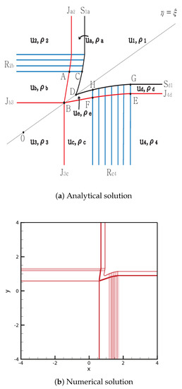
Figure 10. Case 8. SJ + RJ + JR + JS.

Case 9.

$JR+JS+RJ+SJ(u_2<u_1<u_3<u_4<0)$

From the initial discontinuity, contact rarefaction is formed at the positive $\eta$-axis and negative $\eta$-axis, and contact shock is formed at the negative $\xi$-axis and positive $\xi$-axis. $J_{2b}$ completely penetrates $R_{a2}$, and the straight contact discontinuity $J_{ae}$ continues from $A(2u_1,\frac{2u_1{u}_2-u_1^2}{u_2})$ to the singular point $B(u_1,u_1)$. The shock $S_{b3}$ completely penetrates the rarefaction wave $R_{a2}$, and the straight shock $S_{e3}$ continues from $C(2u_1,\frac{u_1^2+u_3^2-2u_1{u}_2}{u_3-u_2})$ to the singular point $D(u_1+u_3,u_1+u_3)$.

By contrast, $J_{c4}$ intersects with $S_{4d}$ at point $E(u_4,u_4+u_1)$, and the new contact discontinuity $J_{ed}$ from E stops at the singular point B. Therefore, four contact discontinuities $J_{a1},J_{ae},J_{ed}$, and $J_{d1}$ meet at the singular point B. The shock $S_{ce}(=S_{4d})$ penetrates the entire rarefaction wave $R_{3c}$, and the straight shock $S_{3e}$ continues from $F(2u_3,\frac{u_1^2+u_3^2-2u_3{u}_4}{u_1-u_4})$ to the singular point D. The solutions are shown in Figure 11. The initial condition is $u_1=-0.43,u_2=-0.56,u_3=-0.37,u_4=-0.15.$

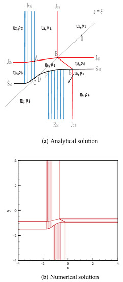
Figure 11. Case 9. JR + JS + RJ + SJ.

Case 10.

$SJ+RJ+JS+JR(0<u_4<u_3<u_1<u_2)$

From the initial discontinuity, contact shock is formed at the positive $\eta$-axis and negative $\eta$-axis, and contact rarefaction is formed at the negative $\xi$-axis and positive $\xi$-axis. $J_{a2}$ completely penetrates $R_{2b}$, and the straight contact discontinuity $J_{eb}$ continues from $A(\frac{2u_2{u}_3-u_3^2}{u_2},2u_3)$ to the singular point $B(u_3,u_3)$. The shock $S_{1a}$ meets the rarefaction wave $R_{2b}$ at point $C(u_1+u_2,2u_2)$, and the curved shock continues to point $D(2u_1,2u_1)$. Both rarefaction waves $R_{2b}$ and $R_{d1}$ meet at $(2u,2u)$ for $u_3\le u\le u_1$ between $E(2u_3,2u_3)$ and D.

By contrast, $J_{4d}$ intersects with $S_{c4}$ at point $F(u_3+u_4,u_4)$, and $J_{ce}$ stops at the singular point B. Therefore, four contact discontinuities $J_{eb},J_{b3},J_{3c}$, and $J_{ce}$ meet at the singular point B. The shock $S_{ed}(=S_{c4})$ meets the rarefaction wave $R_{d1}$ at point $G(u_3+u_4,2u_4)$, and the curved shock then continues to point E. The solutions are shown in Figure 12. The initial condition is $u_1=0.43,u_2=0.56,u_3=0.37,u_4=0.15.$

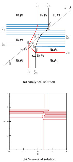
Figure 12. Case 10. SJ + RJ + JS + JR.

Case 11.

$JS+JR+RJ+SJ(u_1<u_3<u_2<u_4<0)$

From the initial discontinuity, contact shock is formed at the positive $\eta$-axis and positive $\xi$-axis, and contact rarefaction is formed at the negative $\xi$-axis and negative $\eta$-axis. $J_{2b}$ meets $S_{a2}$ at point $A(u_1+u_2,u_2)$, and $J_{ae}$ stops at the singular point $B(u_1,u_1)$. The shock $S_{eb}(=S_{a2})$ completely penetrates $R_{b3}$ and stops at the singular point $D(u_1+u_3,u_1+u_3)$.

By contrast, $J_{c4}$ intersects with $S_{4d}$ at point $C(u_4,u_4+u_1)$, and $J_{ed}$ stops at the singular point B. Thus, four contact discontinuities $J_{1a},J_{ae},J_{ed}$, and $J_{d1}$ meet at the singular point B. The shock $S_{ce}(=S_{4d})$ completely penetrates $R_{3c}$ and stops at the singular point D. The solutions are shown in Figure 13. The initial condition is $u_1=-0.56,u_2=-0.37,$$u_3=-0.43,u_4=-0.15.$

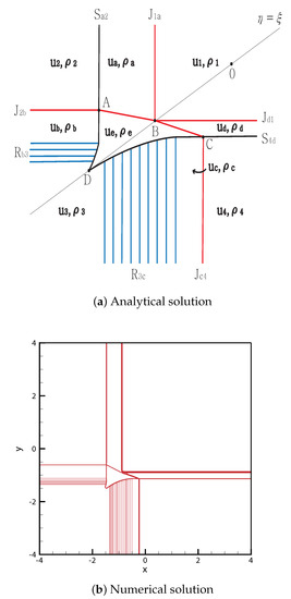
Figure 13. Case 11. JS + JR + RJ + SJ.

Case 12.

$JS+JR+RJ+SJ(u_3<u_1<u_4<u_2<0)$

In this case, the exterior waves at the initial discontinuity were exactly the same as those in Case 11. $J_{2b}$ intersects with $S_{a2}$ at point $A(u_1+u_2,u_2)$, and $J_{ae}$ stops at the singular point $B(u_1,u_1)$. The shock $S_{eb}(=S_{a2})$ meets the rarefaction wave $R_{b3}$ at point $C(u_1+u_2,2u_2)$, and the curved shock then continues to point $D(2u_1,2u_1)$. Both rarefaction waves $R_{b3}$ and $R_{3c}$ meet at $(2u,2u)$ for $u_3\le u\le u_1$ between $E(2u_3,2u_3)$ and D.

By contrast, $J_{c4}$ intersects with $S_{4d}$ at point $F(u_4,u_4+u_1)$, and $J_{ed}$ stops at the singular point B. Thus, four contact discontinuities $J_{1a},J_{ae},J_{ed}$, and $J_{d1}$ meet at the singular point B. The shock $S_{ce}(=S_{4d})$ meets the rarefaction wave $R_{3c}$ at point $G(2u_4,u_4+u_1)$, and the curved shock then continues to point D. The solutions are shown in Figure 14. The initial condition is $u_1=-0.43,u_2=-0.15,u_3=-0.56,u_4=-0.21.$

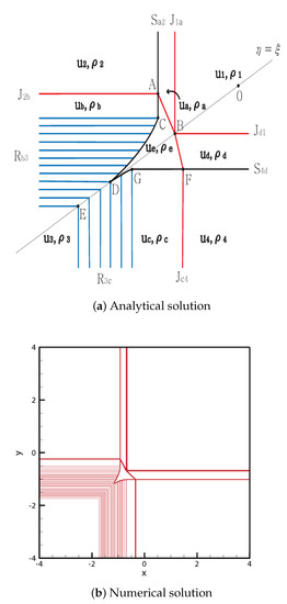
Figure 14. Case 12. JS + JR + RJ + SJ.

Case 13.

$JR+JS+SJ+RJ(u_2<u_4<u_3<u_1<0)$

From the initial discontinuity, contact rarefaction is formed at the positive $\eta$-axis and positive $\xi$-axis, and contact shock is formed at the negative $\xi$-axis and negative $\eta$-axis. $J_{2b}$ completely penetrates $R_{a2}$, and the straight contact discontinuity continues from $A(2u_1,\frac{2u_1{u}_2-u_1^2}{u_2})$ to the singular point $B(u_1,u_1)$. The shock $S_{b3}$ meets the rarefaction wave $R_{a2}$ at point $C(2u_2,u_2+u_3)$, and the curved shock continues to point $D(2u_3,2u_3)$. Both rarefaction waves $R_{a2}$ and $R_{4d}$ meet at $(2u,2u)$ for $u_3\le u\le u_1$ between D and $E(2u_1,2u_1)$.

By contrast, $S_{3c}$ meets $R_{ce}(=R_{4d})$ at point $F(u_3+u_4,2u_4)$, and the curved shock then continues to point D. $J_{c4}$ completely penetrated $R_{4d}$, and the straight contact discontinuity continued from $G(\frac{2u_1{u}_4-u_1^2}{u_4},2u_1)$ to B, which is a singular point of the four contact discontinuities $J_{1a},J_{ae},J_{ed}$, and $J_{d1}$. The solutions are shown in Figure 15. The initial condition is $u_1=-0.15,u_2=-0.56,u_3=-0.21,u_4=-0.43.$

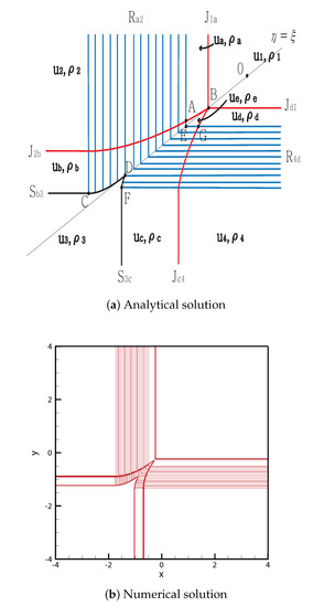
Figure 15. Case 13. JR + JS + SJ + RJ.

Case 14.

$R+JS+R+JS(u_2<u_3<0<u_1<u_4)$

From the initial discontinuity, rarefaction is formed at the positive $\eta$-axis and negative $\eta$-axis, and contact shock is formed at the negative $\xi$-axis and positive $\xi$-axis. The contact discontinuity $J_{2b}$ meets the rarefaction wave $R_{12}$ at point $A(2u_2,u_2)$, and the curved contact continues to point $O(0,0)$. $S_{b3}$ meets $R_{12}$ at point $B(2u_2,u_2+u_3)$, and the curved shock continues to point $C(2u_3,2u_3)$. Both rarefaction waves $R_{12}$ and $R_{34}$ meet at $(2u,2u)$ for $u_3\le u\le u_1$ between C and $D(2u_1,2u_1)$.

By contrast, $J_{4d}$ meets the rarefaction wave $R_{34}$ at point $E(2u_4,u_4)$, and the curved contact discontinuity then continues to point O. $S_{d1}$ meets $R_{34}$ at point $F(2u_4,u_4+u_1)$; the curved shock then continues to point D. The solutions are shown in Figure 16. The initial condition is $u_1=0.43,u_2=-0.37,u_3=-0.15,u_4=0.56.$

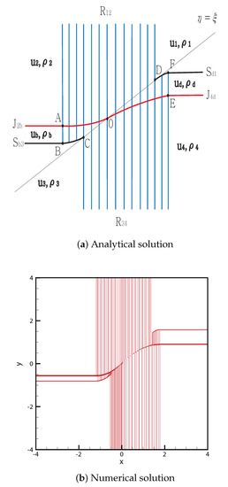
Figure 16. Case 14. R + JS + R + JS.

Case 15.

$SJ+R+R+JS(u_3<0<u_1<u_2<u_4)$

From the initial discontinuity, contact shock is formed at the positive $\eta$-axis and positive $\xi$-axis, and rarefaction is formed at the negative $\xi$-axis and negative $\eta$-axis. The contact discontinuity $J_{a2}$ meets the rarefaction wave $R_{23}$ at point $A(u_2,2u_2)$, and the curved contact then continues to point $O(0,0)$. $S_{1a}$ meets $R_{23}$ at point $B(u_1+u_2,2u_2)$, and the curved shock continues to point $C(2u_1,2u_1)$. Both rarefaction waves $R_{23}$ and $R_{34}$ meet at $(2u,2u)$ for $u_3\le u\le u_1$ between $D(2u_3,2u_3)$ and C.

By contrast, $J_{4d}$ meets the rarefaction wave $R_{34}$ at point $E(2u_4,u_4)$, and the curved contact discontinuity then continues to point O. $S_{d1}$ meets $R_{34}$ at point $F(2u_4,u_4+u_1)$, and the curved shock continues to point C. The solutions are shown in Figure 17. The initial condition is $u_1=0.21,u_2=0.43,u_3=-0.15,u_4=0.56.$

Figure 17. Case 15. SJ + R + R + JS.

3.4. Three Shocks

$$\begin{array}{c}Case16:\left\{\begin{array}{c}SJ+RJ+JS+JS\left(01432\right),SJ+SJ+JR+JS\left(01234\right)\hfill \\ JR+JS+SJ+SJ\left(21430\right),JS+JS+SJ+RJ\left(41230\right)\hfill \end{array}\right.\hfill \\ Case17:\left\{\begin{array}{c}RJ+SJ+JS+JS\left(02143\right),SJ+SJ+JS+JR\left(04123\right)\hfill \\ JS+JS+RJ+SJ\left(12340\right),JS+JR+SJ+SJ\left(14320\right)\hfill \end{array}\right.\hfill \end{array}$$

Case 16.

$SJ+RJ+JS+JS(0<u_1<u_4<u_3<u_2)$

From the initial discontinuity, contact rarefaction is formed at the negative $\xi$-axis, and contact shock is formed at the remaining three axes. The contact discontinuity $J_{a2}$ completely penetrates $R_{2b}$ and stops at the singular point $C(u_3,u_3)$. The shock $S_{1a}$ penetrates the entire rarefaction wave $R_{2b}$, and the straight shock $S_{1e}$ continues from $E(\frac{u_1^2+u_3^2-2u_2{u}_3}{u_1-u_2},2u_3)$ to the singular point $F(u_1+u_3,u_1+u_3)$.

By contrast, $J_{4d}$ intersects with the shock $S_{c4}$ at point $G(u_3+u_4,u_4)$, and the new contact discontinuity $J_{ce}$ from G meets three contact discontinuities, $J_{eb},J_{b3}$, and $J_{3c}$, at the singular point C. The shock $S_{ed}(=S_{c4})$ meets $S_{d1}$ at point $H(u_3+u_4,u_4+u_1)$, and the new shock $S_{e1}$ from H then meets the shock $S_{1e}$ at the singular point F. The solutions are shown in Figure 18. The initial condition is $u_1=0.15,u_2=0.56,u_3=0.43,u_4=0.37.$

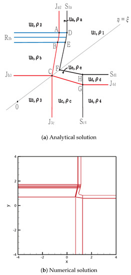
Figure 18. Case 16. SJ + RJ + JS + JS.

Case 17.

$SJ+SJ+JS+JR(0<u_4<u_1<u_2<u_3)$

From the initial discontinuity, contact rarefaction is formed at the positive $\xi$-axis, and contact shock is formed at the remaining three axes. $J_{a2}$ intersects with $S_{2b}$ at point $A(u_2,u_2+u_3)$, and $J_{eb}$ ends at the singular point $B(u_3,u_3)$. The shock $S_{ae}(=S_{2b})$ meets $S_{1a}$ at point $C(u_1+u_2,u_2+u_3)$, and the new shock $S_{1e}$ ends at the singular point $D(u_1+u_3,u_1+u_3)$.

By contrast, $J_{4d}$ intersects with $S_{c4}$ at point $E(u_3+u_4,u_4)$, and $J_{ce}$ ends at the singular point B. Therefore, four contact discontinuities, $J_{eb},J_{b3},J_{3c}$, and $J_{ce}$, meet at the singular point B. The shock $S_{ed}(=S_{c4})$ meets the rarefaction wave $R_{d1}$ at point $F(u_3+u_4,2u_4)$, and the curved shock continues to G. The curved shock from F to G satisfies the following:

$$\frac{d\eta }{d\xi }=\frac{\eta -(u+u_3)}{\xi -(u+u_3)},\eta =2u,\frac{\rho }{u}=\frac{{\rho }_1}{u_1},u_4\le u\le u_1,$$

(21)

and we obtain

$$\xi =\eta +\frac{1}{u_3-u_4}{\left(\frac{\eta }{2}-u_3\right)}^2,2u_4\le \eta \le 2u_1.$$

(22)

The straight shock $S_{e1}$ from point $G(\frac{u_1^2+u_3^2-2u_1{u}_4}{u_3-u_4},2u_1)$ meets $S_{1e}$ at the singular point D. The solutions are shown in Figure 19. The initial condition is $u_1=0.37,u_2=0.43,$$u_3=0.56,u_4=0.15.$

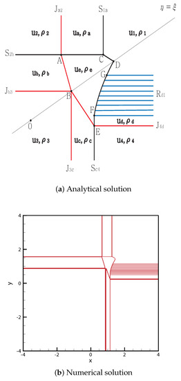
Figure 19. Case 17. SJ + SJ + JS + JR.

3.5. Four Shocks

$$Case18:SJ+SJ+JS+JS(01243,01423),JS+JS+SJ+SJ(12430,14230)$$

Case 18.

$SJ+SJ+JS+JS(0<u_1<u_2<u_4<u_3)$

From the initial discontinuity, contact shocks were formed at each discontinuity. $J_{a2}$ intersects with the shock $S_{2b}$ at point $A(u_2,u_2+u_3)$, and $J_{eb}$ ends at the singular point $B(u_3,u_3)$. The shock $S_{ae}(=S_{2b})$ meets $S_{1a}$ at point $C(u_1+u_2,u_2+u_3)$, and the new shock $S_{1e}$ ends at the singular point $D(u_1+u_3,u_1+u_3)$.

By contrast, $J_{4d}$ intersects with $S_{c4}$ at point $E(u_3+u_4,u_4)$ and $J_{ce}$ meets three contact discontinuities $J_{eb},J_{b3}$, and $J_{3c}$ at the singular point B. The shock $S_{ed}(=S_{c4})$ meets $S_{d1}$ at point $F(u_3+u_4,u_4+u_1)$. The new shock $S_{e1}$ from F meets the shock $S_{1e}$ at the singular point D. The solutions are shown in Figure 20. The initial condition is $u_1=0.15,$$u_2=0.37,u_3=0.56,u_4=0.43.$

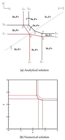
Figure 20. Case 18. SJ + SJ + JS + JS.

4. Discussion

The solutions are separated into 14 cases [34] in which delta shock appears at the initial discontinuity and 18 cases in which delta shock did not appear. Because we remove the assumption $\left(H\right)$, there is either one or two waves at each initial discontinuity. If the values of u on either side of the initial discontinuity have the same sign, then there are two waves: contact shock $\left(JS\right)$ or contact rarefaction $\left(JR\right)$. If they have different signs, then there is only one wave, either delta shock $\left(S_{\delta }\right)$ or rarefaction $\left(R\right)$.

For 14 cases in [34], due to the delta shock, there is always one wave solution. They are classified into six cases of two delta shocks $(S_{\delta }+S_{\delta })$, six cases of one delta shock and one rarefaction $(S_{\delta }+R)$, and two cases of two delta shocks and two rarefactions $(S_{\delta }+S_{\delta }+R+R)$. Because each case includes one wave solution, they provide a relatively simple wave interaction structure. Conversely, in this study, we have 18 cases that include only six cases of two rarefactions $(R+R)$ as one wave solution. This means that 12 cases involve two waves $\left(JS\mathrm{or}JR\right)$ at each initial discontinuity, and they show a relatively complicated wave interaction structure.

5. Conclusions

We consider a four-quadrant RP for system (3) without the assumption that each jump of the initial data projects exactly one planar elementary wave. The main results of this study include the classification of the solution and the construction of analytic and numerical solutions for each case. In [34], we considered a case involving delta shock appearing at the initial discontinuity. It was separated into 52 cases, resulting in 14 solutions. In this paper, we considered initial data that do not involve delta shock, and it is separated into 68 cases, resulting in 18 solutions. Hence, a four-quadrant RP for system (3) classified a total of 32 topologically distinct solutions.

Because no general theory exists for systems in multiple space dimensions, 2-D RP for systems must be investigated on a case-by-case basis. Furthermore, the theory provides little insight into the qualitative behavior of wave interactions. Therefore, to understand the qualitative behavior of the structures in wave interactions of the Riemann problem, we need to construct the solutions of each individual system.

In both studies, all analytic solutions and numerical solutions of the four-quadrant RP for system (3) are constructed; the numerical solutions are remarkably coincident with the constructed analytic solutions. The results show the rich structures of the wave interactions of RP and interesting phenomena.

References

- Conway, E.; Smoller, J. Global solutions of the Cauchy problem for quasi-linear first-order equations in several space variables. Commun. Pure Appl. Math. 1966, 19, 95–105. [Google Scholar] [CrossRef]
- Kruzkov, S.N. First order quasilinear equations in several independent variables. Math. USSR-Sbornik. 1970, 10, 217–243. [Google Scholar] [CrossRef]
- Val’ka, Y. Discontinuous solutions of a multidimensional quasilinear equation (numerical experiments). USSR Comput. Math. Math. Phys. 1968, 8, 257–264. [Google Scholar] [CrossRef]
- Vol’pert, A.I. The spaces BV and quasilinear equations. Mat. Sb. 1967, 115, 255–302. [Google Scholar]
- Guckenheimer, J. Shocks and rarefactions in two space dimensions. Arch. Rarefactionn. Mech. Anal. 1975, 59, 281–291. [Google Scholar] [CrossRef]
- Wagner, D.H. The Riemann problem in two space dimensions for a single conservation law. SIAM J. Math. Anal. 1983, 14, 534–559. [Google Scholar] [CrossRef]
- Lindquist, W.B. The scalar Riemann problem in two spatial dimensions: Piecewise smoothness of solutions and its breakdown. SIAM J. Math. Anal. 1986, 17, 1178–1197. [Google Scholar] [CrossRef]
- Lindquist, W.B. Construction of solutions for two-dimensional Riemann problems. In Hyperbolic Partial Differential Equations; Elsevier: Amsterdam, The Netherlands, 1986; pp. 615–630. [Google Scholar]
- Glimm, J.; Klingenberg, C.; McBryan, O.; Plohr, B.; Sharp, D.; Yaniv, S. Front tracking and two-dimensional Riemann problems. Adv. Appl. Math. 1985, 6, 259–290. [Google Scholar] [CrossRef]
- Zhang, T.; Zheng, Y.X. Conjecture on the structure of solutions of the Riemann problem for two-dimensional gas dynamics systems. SIAM J. Math. Anal. 1990, 21, 593–630. [Google Scholar] [CrossRef]
- Chen, T.; Qu, A. Two-dimensional Riemann problem for Chaplygin gas dynamics in four pieces. J. Math. Anal. Appl. 2017, 448, 580–597. [Google Scholar] [CrossRef]
- Cheng, H.; Liu, W.; Yang, H. Two-dimensional Riemann problems for zero-pressure gas dynamics with three constant states. J. Math. Anal. Appl. 2008, 343, 127–140. [Google Scholar] [CrossRef][Green Version]
- Pang, Y.; Tian, J.P.; Yang, H. Two-dimensional Riemann problem for a hyperbolic system of conservation laws in three pieces. Appl. Math. Comput. 2012, 219, 1695–1711. [Google Scholar] [CrossRef]
- Pang, Y.; Tian, J.P.; Yang, H. Two-dimensional Riemann problem involving three J’s for a hyperbolic system of nonlinear conservation laws. Appl. Math. Comput. 2013, 219, 4614–4624. [Google Scholar] [CrossRef]
- Shen, C. Riemann problem for a two-dimensional quasilinear hyperbolic system. Electron. J. Differ. Equ. 2015, 2015, 1–13. [Google Scholar]
- Shen, C.; Sun, M. The Riemann problem for the pressure-gradient system in three pieces. Appl. Math. Lett. 2009, 22, 453–458. [Google Scholar] [CrossRef][Green Version]
- Sheng, W.; Zhang, T. The Riemann Problem for the Transportation Equations in Gas Dynamics; American Mathematical Society: Providence, RI, USA, 1999; Volume 654. [Google Scholar]
- Tan, D.C.; Zhang, T. Two-dimensional Riemann problem for a hyperbolic system of nonlinear conservation laws: I. four-J cases. J. Differ. Equ. 1994, 111, 203–254. [Google Scholar] [CrossRef]
- Tan, D.C.; Zhang, T. Two-dimensional Riemann problem for a hyperbolic system of nonlinear conservation laws: II. Initial data involving some rarefaction waves. J. Differ. Equ. 1994, 111, 255–282. [Google Scholar] [CrossRef]
- Wang, G.; Chen, B.; Hu, Y. The two-dimensional Riemann problem for Chaplygin gas dynamics with three constant states. J. Math. Anal. Appl. 2012, 393, 544–562. [Google Scholar] [CrossRef]
- Zhang, P.; Li, J.; Zhang, T. On two-dimensional Riemann problem for pressure-gradient equations of the Euler system. Discret. Contin. Dyn. Syst. 1998, 4, 609–634. [Google Scholar] [CrossRef]
- Chang, T.; Hsiao, L. The Riemann problem and interaction of waves in gas dynamics. NASA STI/Recon Tech. Rep. A 1989, 90, 44044. [Google Scholar]
- Quan, L.; Li, Y.; Zhang, T. The Two-Dimensional Riemann Problem in Gas Dynamics; CRC Press: Boca Raton, FL, USA, 1998. [Google Scholar]
- Zheng, Y. Systems of Conservation Laws: Two-Dimensional Riemann Problems; Springer Science Business Media: Berlin/Heidelberg, Germany, 2012. [Google Scholar]
- Yang, H. Generalized plane delta-shock waves for n-dimensional zero-pressure gas dynamics. J. Math. Anal. Appl. 2001, 260, 18–35. [Google Scholar] [CrossRef]
- Hwang, W.; Lindquist, W.B. The 2-dimensional Riemann problem for a 2×2 hyperbolic conservation law I. Isotropic media. SIAM J. Math. Anal. 2002, 34, 341–358. [Google Scholar] [CrossRef]
- Hwang, W.; Lindquist, W.B. The 2-dimensional Riemann problem for a 2×2 hyperbolic conservation law II. Anisotropic media. SIAM J. Math. Anal. 2002, 34, 359–384. [Google Scholar] [CrossRef]
- Shen, C.; Sun, M.; Wang, Z. Global structure of Riemann solutions to a system of two-dimensional hyperbolic conservation laws. Nonlinear Anal. 2011, 74, 4754–4770. [Google Scholar] [CrossRef]
- Sun, M. Construction of the 2D Riemann solutions for a nonstrictly hyperbolic conservation law. Bull. Korean Math. Soc. 2013, 50, 201–216. [Google Scholar] [CrossRef]
- Hwang, J.; Shin, M.; Shin, S.; Hwang, W. Two dimensional Riemann problem for a 2×2 system of hyperbolic conservation laws involving three constant states. Appl. Math. Comput. 2018, 321, 49–62. [Google Scholar] [CrossRef]
- Isaacson, E.L. Global Solution of a Riemann Problem for a Non-Strictly Hyperbolic System of Conservation Laws Arising in Enhanced Oil Recovery; Enhanced Oil Recovery Institute, University of Wyoming: Laramie, WY, USA, 1989. [Google Scholar]
- Keyfitz, B.L.; Kranzer, H.C. A system of non-strictly hyperbolic conservation laws arising in elasticity theory. Arch. Rat. Mech. Anal. 1980, 72, 219–241. [Google Scholar] [CrossRef]
- Temple, B. Global solution of the Cauchy problem for a class of 2×2 nonstrictly hyperbolic conservation laws. Adv. Appl. Math. 1982, 3, 335–375. [Google Scholar] [CrossRef]
- Hwang, J.; Shin, S.; Shin, M.; Hwang, W. Four-quadrant Riemann problem for a 2×2 system involving delta shock. Mathematics 2021, 9, 138. [Google Scholar] [CrossRef]
- Kurganov, A.; Lin, C.T. On the reduction of numerical dissipation in central-upwind schemes. Commun. Comput. Phys 2007, 2, 141–163. [Google Scholar]
- Shin, M.; Shin, S.; Hwang, W. A treatment of contact discontinuity for central upwind scheme by changing flux functions. J. Korean Soc. Ind. Appl. Math. 2013, 17, 29–45. [Google Scholar] [CrossRef][Green Version]
Publisher’s Note: MDPI stays neutral with regard to jurisdictional claims in published maps and institutional affiliations. |
© 2021 by the authors. Licensee MDPI, Basel, Switzerland. This article is an open access article distributed under the terms and conditions of the Creative Commons Attribution (CC BY) license (http://creativecommons.org/licenses/by/4.0/).