A High Order Accurate and Effective Scheme for Solving Markovian Switching Stochastic Models

Abstract

In this paper, we propose a new weak order 2.0 numerical scheme for solving stochastic differential equations with Markovian switching (SDEwMS). Using the Malliavin stochastic analysis, we theoretically prove that the new scheme has local weak order 3.0 convergence rate. Combining the special property of Markov chain, we study the effects from the changes of state space on the convergence rate of the new scheme. Two numerical experiments are given to verify the theoretical results.

1. Introduction

In recent years, stochastic differential equations with Markovian switching (SDEwMS) has attracted the attention of many scholars. Comparing with stochastic differential equations with jumps (SDEwJ), SDEwMS are not only applied in finance, but they also have many applications in other fields, which include control system, biomathematics, chemistry, and mechanics. Zhou and Mamon [1] proposed an accessible implementation of interest rate models with Markov-switching. Siu [2] proposed a high-order Markov-switching model for risk measurement. He, Qi, and Kao [3] studied the HMM-based adaptive attack-resilient control for Markov jump system and application to an aircraft model. In this paper, we consider the following q-dimensional stochastic differential equations with Markovian switching:

$$d{X}_s=a(s,r_s,X_s)ds+b(s,r_s,X_s)d{W}_s,0\le s\le T,$$

(1)

where $r_s\in \mathbb{S}$, the Brownian motion $W_s={(W_s^1,W_s^2,\dots ,W_s^m)}_{s\ge 0}^T,$ is independent of the Markov chain $r_t(t\ge 0)$, $a:[0,T]\times \mathbb{S}\times {\mathbb{R}}^q⟶{\mathbb{R}}^q$ and $b:[0,T]\times \mathbb{S}\times {\mathbb{R}}^q⟶{\mathbb{R}}^{q\times m}$. Qualitative theory of the existence and uniqueness of the solution for SDEwMS has been studied for the past years (see [4,5]). Many scholars have studied the stability of SDEwMS, for example, stability of linear or semi-linear type of Equation (1) has been studied by Basak [6] and Ji [7]. Mao [4] discussed the exponential stability for general nonlinear stochastic differential equations with Markovian switching. Yang, Yin and Li [8] focused on stability analysis of numerical solutions to jump diffusion and jump diffusion with Markovian switching. Ma and Jia [9] considered the stability analysis of linear It$\widehat{o}$ stochastic differential equations with countably infinite Markovian switchings.

Generally, most of SDEwMS do not have explicit solutions and hence require numerical solutions. Yuan and Mao [10] firstly developed a Euler–Maruyama scheme for solving SDEwMS and estimated the errors between the numerical and exact solutions under Lipschitz conditions. Yuan and Mao [11] proved that the strong rate of convergence of the Euler–Maruyama scheme is equal to 0.5 under non-Lipschitz conditions. Then, many scholars extended to the semi-implicit Euler scheme [12,13,14]. Furthermore, Li [15] and Chen [16] developed an Euler scheme for solving stochastic differential equations with Markovian switching and jumps. For a higher convergence rate, many scholars aimed to design a numerical Milstein-type scheme. Fan [17] and Nguyen [18] proposed the Milstein scheme for solving SDEwMS and proved its strong rate of convergence is equal to 1.0. Based on the work of Author1 [18], Kumar [19] provided many improved conditions to prove the convergence theorem of Milstein scheme. Lately, Zhao [20] proposed a two-step Euler scheme for solving highly nonlinear SDEwMS.

Since Markov chain is a special Poisson jump process, the numerical scheme for solving SDEwJ can be applied to solve SDEwMS. There are some scholars studying in higher order weak numerical schemes for solving SDEwJ. For example, Buckwar [21] proposed the implicit order 2.0 Runge–Kutta scheme for solving jump-diffusion differential equations. Liu and Li [22] studied an effective higher order weak scheme to solve stochastic differential equations with jumps but involved computing multiple stochastic integral. Lately, Author1 [23] proposed a new simplified weak order 2.0 scheme for solving stochastic differential equations with Poisson jumps.

Inspired by high-order numerical methods [21,22,23] and based on classical weak order 2.0 Taylor scheme [24] for solving stochastic differential equations, we develop a new weak order 2.0 numerical approximation scheme for solving SDEwMS and rigorously prove the new scheme has order 2.0 convergence rate by using Malliavin stochastic analysis. Meanwhile, we simply utilize the Runge–Kutta scheme for solving SDEwMS in order to make a comparison with the new scheme on the accuracy and convergence rate. In addition, in view of the special property of Markov chain, we fully investigate the effects from the state space of Markov chain on the convergence rate of the new scheme.

The important contributions of this paper can now be highlighted as follows:

• We propose a new weak order 2.0 scheme and approximate multiple stochastic integral by utilizing the compound Poisson process.
• By integration-by-parts formula of Malliavin calculus theory [25], we rigorously prove that the new scheme has local weak order 3.0 convergence rate. We also prove that the convergence rate is related to the maximum state difference and upper bounds of state values.
• We give two numerical experiments to confirm our theoretical convergence results and the convergence rate effects from Markov chain space.
• In the experiments, we make comparisons with other schemes such as Euler scheme and Runge–Kutta scheme and verify the new scheme is effective and accurate.

Some notations to be used later are listed as follows:

• $|·|$ is the norm for vector or matrix defined by ${\left|A\right|}^2=\mathrm{trace}\left(A^{T}A\right)$.
• $C_p^k({\mathbb{R}}^q,\mathbb{R})$ is the set of k times continuously differentiable functions which, together with their partial derivatives of order up to k, have at most polynomial growth.
• ${\mathcal{F}}_s$$(t\le s\le T)$ is the $\sigma$-field generated by the diffusion process $\{X_s,t\le s\le T\}$.
• C is a generic constant depending only on the upper bounds of derivatives of $a,b$ and g, and C can be different from line to line.

The paper is organized as follows. In Section 2, we introduce some basic concepts. In Section 3, we propose a new scheme and obtain its local order 3.0 convergence results. In Section 4, two numerical examples are given to verify the theoretical results.

2. Preliminaries

2.1. Markov Chain

In this paper, let $(\mathsf{\Omega },\mathcal{F},{\left\{{\mathcal{F}}_t\right\}}_{t\ge 0},P)$ be a complete probability space with a filtration ${\left\{{\mathcal{F}}_t\right\}}_{t\ge 0}$ satisfying the usual conditions. Let ${\mathbf{x}}^{\mathbf{T}}$ denote the transpose of a vector or matrix $\mathbf{x}$. Let $\left\{r_t,t\ge 0\right\}$ be a right-continuous Markov chain on the probability space taking values in a finite state space $\mathbb{S}=\{1,2,...,M\}$ with generator $Q={\left(q_{ij}\right)}_{M\times M}$ given by

$$P(r_{t+\delta }=j|r_t=i)=\left\{\begin{array}{c}{q}_{ij}\delta +o\left(\delta \right),\mathrm{if}i\ne j,\hfill \\ 1+q_{ii}\delta +o\left(\delta \right),\mathrm{if}i=j,\hfill \end{array}\right.$$

(2)

where $\delta >0$, $q_{ij}\ge 0$ and, for $i\ne j$, $q_{ii}=-{\displaystyle \sum _{i\ne j}}{q}_{ij}.$ For the above Markov chain, $N(de,dt)$ is a Poisson random measure with intensity $\lambda \left(de\right)dt$ on $\mathcal{E}\times [0,T]$, in which $\lambda$ is the Lebesgue measure on $\mathcal{E}$, where $\mathcal{E}=\mathbb{R}\backslash \left\{0\right\}$ is equipped with its Borel field E. $d{r}_t={\int }_{\mathcal{E}}l(r_{t-},e)N(de,dt)$ with $l(i,e)=j-ifore\in {\mathsf{\Delta }}_{ij}andl(i,e)=0fore\notin {\mathsf{\Delta }}_{ij},$ where ${\mathsf{\Delta }}_{ij}$ are the intervals having length $q_{ij}$ satisfying

$$\begin{array}{cc}\hfill & {\mathsf{\Delta }}_{12}=[0,q_{12}),{\mathsf{\Delta }}_{13}=[q_{12},q_{12}+q_{13}),...,{\mathsf{\Delta }}_{1M}=[{\displaystyle \sum _{j=2}^{M-1}}{q}_{1j},{\displaystyle \sum _{j=2}^M}{q}_{1j}),\hfill \\ \hfill & {\mathsf{\Delta }}_{21}=[{\displaystyle \sum _{j=2}^M}{q}_{1j},{\displaystyle \sum _{j=2}^M}{q}_{1j}+q_{21}),{\mathsf{\Delta }}_{23}=[{\displaystyle \sum _{j=2}^M}{q}_{1j}+q_{21},{\displaystyle \sum _{j=2}^M}{q}_{1j}+q_{21}+q_{23}),...,\hfill \\ \hfill & {\mathsf{\Delta }}_{2M}=[{\displaystyle \sum _{j=2}^M}{q}_{1j}+{\displaystyle \sum _{\genfrac{}{}{0pt}{}{j=1,}{j\ne 2}}^{M-1}}{q}_{2j},{\displaystyle \sum _{j=2}^M}{q}_{1j}+{\displaystyle \sum _{\begin{array}{c}j=1\\ j\ne 2\end{array}}^M}{q}_{2j}),...,\hfill \end{array}$$

and so on.

In [17], the discrete Markov chain $\{r_{nh},n=0,1,...\}$ given a step size $h>0$ is simulated as follows: compute the one-step transition probability matrix

$$\begin{array}{cc}\hfill & P\left(h\right)={\left(P_{i,j}\left(h\right)\right)}_{M\times M}=e^{hQ}.\hfill \end{array}$$

Let $r_0=i_0$ and generate a random number ${\xi }_1$ which is uniformly distributed in $[0,1]$. Define

$$r_h=\left\{\begin{array}{c}{i}_1,\mathrm{if}{i}_1\in \mathbb{S}-\left\{M\right\}suchthat{\displaystyle \sum _{j=1}^{i_1-1}}{P}_{i_0,j}\left(h\right)\le {\xi }_1\le {\displaystyle \sum _{j=1}^{i_1}}{P}_{i_0,j}\left(h\right),\hfill \\ M,\mathrm{if}{\displaystyle \sum _{j=1}^{M-1}}{P}_{i_0,j}\left(h\right)\le {\xi }_1,\hfill \end{array}\right.$$

(3)

where we set ${\displaystyle \sum _{j=1}^0}{P}_{i_0,j}\left(h\right)=0$ as usual. Generate independently a new random number ${\xi }_2$, which is again uniformly distributed in $[0,1]$, and then define

$$r_{2h}=\left\{\begin{array}{c}{i}_2,\mathrm{if}{i}_2\in \mathbb{S}-\left\{M\right\}suchthat{\displaystyle \sum _{j=1}^{i_2-1}}{P}_{r\left(h\right),j}\left(h\right)\le {\xi }_1\le {\displaystyle \sum _{j=1}^{i_2}}{P}_{r\left(h\right),j}\left(h\right),\hfill \\ M,\mathrm{if}{\displaystyle \sum _{j=1}^{N-1}}{P}_{r\left(h\right),j}\left(h\right)\le {\xi }_2.\hfill \end{array}\right.$$

(4)

2.2. It$\widehat{o}$ Formula

Given a multi-index $\alpha \in \mathcal{M}=\{(j_1,j_2,\dots ,j_l):j_i\in \{-1,0,1,\dots ,m\},i\in \{1,\dots ,l\},\mathrm{for}$$l=1,2,3,\dots \}$ with the length $l:=l\left(\alpha \right)\in \{1,2,\dots \}$, we denote the hierarchical set of multi-indices by ${\mathsf{\Gamma }}_m=\left\{\alpha \in \mathcal{M}:l\left(\alpha \right)=m\right\}$ and ${\mathcal{B}}_2=\left\{\alpha =(j_1,j_2)\in \mathcal{M}:1\le j_1,j_2\le m\right\}$. We write $-\alpha$ and $\alpha -$ for the multi-index in $\mathcal{M}$ by deleting the first and last component of $\alpha$, respectively. Denote by $I_{\alpha }{\left[h_{k,\alpha }(·,r_{·},X_{·})\right]}_{\rho ,\tau }$ the multiple Itô integral recursively defined by

$$I_{\alpha }{\left[h_{k,\alpha }(·,r_{·},X_{·})\right]}_{\rho ,\tau }=\left\{\begin{array}{cc}{\int }_{\rho }^{\tau }{I}_{\alpha -}{\left[h_{k,\alpha }(·,r_{·},X_{·})\right]}_{\rho ,s}ds,\hfill & l\ge 1,j_l=0,\hfill \\ {\int }_{\rho }^{\tau }{I}_{\alpha -}{\left[h_{k,\alpha }(·,r_{·},X_{·})\right]}_{\rho ,s}d{W}_s^{j_l},\hfill & l\ge 1,j_l\ge 1,\hfill \\ {\int }_{\rho }^{\tau }{I}_{\alpha -}{\left[h_{k,\alpha }(·,r_{·},X_{·})\right]}_{\rho ,s}d{\tilde{N}}_s,\hfill & l\ge 1,j_l=-1,\hfill \end{array}\right.$$

(5)

where the Itô coefficient functions $h_{k,\alpha }(t,i,x)$ are defined by

$$h_{k,\alpha }(t,i,x)=\left\{\begin{array}{cc}x,\hfill & l=0,\hfill \\ h_{k,\left(0\right)}=a_k(t,i,x),h_{k,\left(j\right)}=b_{k,j}(t,i,x),\hfill & l=1,\hfill \\ L^j{h}_{-\alpha },\hfill & l>1,\hfill \end{array}\right.$$

for all $(t,i,x)\in [0,T]\times \mathbb{S}\times {\mathbb{R}}^q$ and $1\le j\le m$. For $\alpha =(1,1,1)$, we define

$$I_{(0,0,0)}\left[h_{k,\alpha }(·,r_{·},X_{·})\right]={\int }_{t_n}^{t_{n+1}}{\int }_{t_n}^{s_3}{\int }_{t_n}^{s_2}{h}_{k,\alpha }(t_{s_1},r_{s_1},X_{s_1})d{s}_{1}d{s}_{2}d{s}_3.$$

Applied to Equation (1), for $x\in {\mathbb{R}}^q$, $\phi \in C^{2,1}({\mathbb{R}}^q\times \mathbb{S};\mathbb{R})$, we define operators $L^0\phi ,L^j\phi ,L^{-1}\phi$ from ${\mathbb{R}}^q\times \mathbb{S}$ to $\mathbb{R}$,

$$\begin{array}{cc}\hfill & L^0\phi (x,i)={\displaystyle \sum _{j=1}^q}\frac{\partial \phi }{\partial x^j}(x,i)a_j(t,i,x)+\frac{1}{2}{\displaystyle \sum _{j=1}^m}{\displaystyle \sum _{l,k=1}^q}\frac{{\partial }^2\phi }{\partial x^k\partial x^l}(x,i)b_{l,j}(t,i,x)b_{k,j}(t,i,x)+\sum _{j\in S}{q}_{ij}\phi (x,j),\hfill \\ \hfill & L^j\phi (x,i)={\displaystyle \sum _{k=1}^m}\frac{\partial \phi (x,i)}{\partial x^k}{b}_{k,j}(t,i,x),L_e^{-1}\phi (x,i)=\phi (x,i+l(i,e))-\phi (x,i)\hfill \end{array}$$

(6)

for $i\in \mathbb{S}$ and $1\le j\le m$. Then, the It$\widehat{o}$ formula can be presented as:

$$\begin{array}{c}\hfill \phi (X_t,r_t)=\phi (X_0,r_0)+{\int }_0^t{L}^0\phi (X_s,r_s)ds+{\displaystyle \sum _{j=1}^m}{\int }_0^t{L}^j\phi (X_s,r_s)d{W}_s^j+{\int }_0^t{\int }_{\mathcal{E}}{L}_e^{-1}\phi (X_s,r_s)\tilde{N}(de,ds),\end{array}$$

(7)

where $\tilde{N}(de,ds)=N(de,ds)-\lambda \left(de\right)ds$ is a compensated Poisson random measure.

Assumption 1. 

Assume that there exist two positive constants L and K such that

• (Lipschitz condition) for all$x,y\in {\mathbb{R}}^q,t\in [0,T]$and$i\in \mathbb{S}$

  $$\begin{array}{c}\hfill {|a(t,i,x)-a(t,i,y)|}^2{\vee |b(t,i,x)-b(t,i,y)|}^2\le L{|x-y|}^2.\end{array}$$

  (8)
• (Linear growth condition) for all$(t,i,x)\in [0,T]\times \mathbb{S}\times {\mathbb{R}}^q$

  $$\begin{array}{c}\hfill {\left|a(t,i,x)\right|}^2\vee {\left|b(t,i,x)\right|}^2\le {K(1+|x|}^2).\end{array}$$

  (9)

2.3. Malliavin Calculus

Suppose that H is a real separable Hilbert space with scalar product denoted by ${⟨·,·⟩}_H$. The norm of an element $h\in H$ is denoted by ${\parallel h\parallel }_H$. Let $\mathcal{B}=\left\{W\right(h),h\in H\}$ denote an isonormal Gaussian process associated with the Hilbert space H on $(\mathsf{\Omega },\mathcal{F},{\left\{{\mathcal{F}}_t\right\}}_{t\ge 0},P)$.

We call a row vector $\alpha =(j_1,j_2,...j_l)$ with $j_i\in \{-1,0,1,...,m\}$ for $i\in \{1,2,...,l\}$ a multi-index of length $l:l\left(\alpha \right)\in \{1,2,...,m\}$ and denote by v the multi-index of length zero $\left(l\right(v):=0)$. Let $\mathcal{M}$ be the set of all multi-indices, i.e.,

$$\mathcal{M}=\{(j_1,j_2,...,j_l):j_i\in \{-1,0,1,...,m\},i\in \{0,1,...,l\}forl=1,2,...\}\cup \left\{v\right\}.$$

Assume ${\mathsf{\Gamma }}_l=\left\{\alpha |\alpha =(j_1,j_2,...,j_l),j_i\in \{-1,0,1,2,...,m\}\right\}$. We have the following definition

$$D_{s_1...s_l}^{\alpha }=D_{s_1...s_l}^{(j_1,...,j_l)}=D_{s_l}^{j_1}···D_{s_l}^{j_t},$$

where

$$D_{s_i}^{j_i}=\left\{\begin{array}{c}{D}_{s_i}^{-1}{j}_i<0,\hfill \\ D_{s_i}^{j_i}{j}_i>0,\hfill \\ 1,j_i=0.\hfill \end{array}\right.$$

(10)

A random variable F is Malliavin differentiable if and only if $F\in {\mathbb{D}}^{1,2}$, where the space ${\mathbb{D}}^{1,2}\subset L^2\left(P\right)$ is defined by completion with respect to the norm ${\parallel ·\parallel }_{1,2}$. The details about the Malliavin derivative of Poisson process can be found in [25]. For any integer $p\ge 1$, ${\mathbb{D}}^{k,p}$ is the domain of ${\mathbb{D}}^k(k\in \mathbb{N})$ in $L^p\left(\mathsf{\Omega }\right)$, i.e., ${\mathbb{D}}^{k,p}$ is the closure of the class of smooth random variables F with respect to the norm

$${\left|\right|F\left|\right|}_{k,p}^p={\mathbb{E}\left[\right|F|}^p]+{\displaystyle \sum _{j=1}^k}\sum _{\left|\alpha \right|=l}{\int }_0^T...{\int }_0^T\mathbb{E}\left[\right|D_{s_1...s_l}^{\alpha }F{|}^p]d{s}_1...d{s}_l.$$

Lemma 1 (Product rule). 

Let $F,G\in {\mathbb{D}}^{1,2}$, then $FG\in {\mathbb{D}}^{1,2}$, and we have

$$\begin{array}{cc}\hfill & D_t^{-1}\left(FG\right)=F{D}_t^{-1}G+G{D}_t^{-1}F+D_t^{-1}F{D}_t^{-1}G,\hfill \\ \hfill & D_t^1\left(FG\right)=F{D}_t^{1}G+G{D}_t^{1}F.\hfill \end{array}$$

Lemma 2 (Chain rule and Duality formula). 

Let $F\in {\mathbb{D}}^{1,2}$ and $u\left(t\right)\in {\mathbb{D}}^{1,2}$, $0\le t\le T$ and let φ be a real continuous function on $\mathbb{R}$. Then,

$$\begin{array}{cc}& D_t^1\phi \left(F\right)={\displaystyle \sum _{i=1}^q}\frac{\partial \phi }{\partial x_i}\left(F\right)D_t^1{F}_i,D_t^{-1}\phi \left(F\right)=\phi (F+D_t^{-1}F)-\phi \left(F\right),\hfill \\ & \mathbb{E}\left[F{\int }_0^{T}u\left(t\right)d{W}_t\right]=\mathbb{E}\left[{\int }_0^{T}u\left(t\right)D_t^{1}Fdt\right],\mathbb{E}\left[F{\int }_0^T{\int }_{\mathcal{E}}u(t-)\tilde{N}(de,dt)\right]=\mathbb{E}\left[{\int }_0^T{\int }_{\mathcal{E}}u(t-)D_t^{-1}F\lambda \left(de\right)dt\right].\hfill \end{array}$$

3. Main Results

First, we give the equi-step time division; assume $\mathsf{\Delta }t=T/N$, $t_n=n\mathsf{\Delta }t$ for $n=0,1,2,\dots ,N$. For simple representation, we assume $X_{k,t_{n+1}}^{n,i}=X_{k,t_{n+1}}^{t_n,i,X^n}$, which is the kth component of explicit solution $X_{t_{n+1}}^{t_n,i,X^n}$. Assume $\mathsf{\Delta }{B}_n^{-1}={\tilde{N}}_{t_{n+1}}-{\tilde{N}}_{t_n}$, $\mathsf{\Delta }{B}_n^0=t_{n+1}-t_n$, $\mathsf{\Delta }{B}_n^1=W_{t_{n+1}}-W_{t_n}$,

$$J_{\alpha }{[h_{k,\alpha }(·,r_{·},X_{·}^{n,i})]}_{t_n,t_{n+1}}={\int }_{t_n}^{t_{n+1}}{\int }_{t_n}^{t_{n+1}}{h}_{k,\alpha }(s_1,r_{s_1},X_{s_1}^{n,i})d{B}_{s_1}^{j_1}d{B}_{s_2}^{j_2},$$

where multi-index $\alpha =(j_1,j_2)\in {\mathsf{\Gamma }}_2$. Then, it follows from the It$\widehat{o}$–Taylor formula and trapezoidal rule that

$$X_{k,t_{n+1}}^{n,i}=X_k^n+{\int }_{t_n}^{t_{n+1}}{a}_k(s,r_s,X_s^{n,i})ds+{\int }_{t_n}^{t_{n+1}}{b}_k(s,r_s,X_s^{n,i})d{W}_s=X_k^{n+1,i}+R_k^{n+1,i}$$

(11)

with the truncation error

$$R_k^{n+1,i}=\sum _{\alpha \in {\mathcal{A}}_2}\left(I_{\alpha }{\left[h_{k,\alpha }(t_n,i,X^n)\right]}_{t_n,t_{n+1}}-\frac{1}{2}{J}_{\alpha }{\left[h_{k,\alpha }(t_n,i,X^n)\right]}_{t_n,t_{n+1}}\right)+\sum _{\alpha \in {\mathcal{A}}_3}{I}_{\alpha }{\left[h_{k,\alpha }(·,r_{·},X_{·}^{n,i})\right]}_{t_n,t_{n+1}},$$

(12)

where ${\mathcal{A}}_l=\left\{\alpha \right|\alpha =(j_1,j_2,...,j_l),j_i\in \{-1,0,1\},j_l\ne -1\}$. Then, we propose the following weak order 2.0 numerical scheme for solving SDEsMS.

Scheme 1. 

Assume the initial condition$X_0$, $r_0$, applied to Equation (1). For $0\le n\le N-1,$ we have

$$\begin{array}{cc}\hfill X_k^{n+1,i}& =X_k^n+a_k^i\mathsf{\Delta }t+b_k^i\mathsf{\Delta }{W}_n+\frac{1}{2}{L}^0{a}_k^i{\left(\mathsf{\Delta }t\right)}^2+\frac{1}{2}\left(L^1{a}_k^i+L^0{b}_k^i\right)\mathsf{\Delta }t\mathsf{\Delta }{W}_n\hfill \\ \hfill & +\frac{1}{2}\mathsf{\Delta }t{\int }_{t_n}^{t_{n+1}}{\int }_{\mathcal{E}}{L}_e^{-1}{a}_k^i\tilde{N}(de,dt)+\frac{1}{2}{L}^1{b}_k^i({\left(\mathsf{\Delta }{W}_n\right)}^2-\mathsf{\Delta }t)\hfill \\ & +{\int }_{t_n}^{t_{n+1}}{\int }_{t_n}^t{L}_e^{-1}{b}_k^{i}d{N}_{s}d{W}_t-\frac{1}{2}\sum _{j\in \mathbb{S}}(b_k(t_n,j,X^n)-b_k(t_n,i,X^n))q_{ij}\mathsf{\Delta }t\mathsf{\Delta }{W}_n,\hfill \end{array}$$

(13)

where $i=r_{t_n}$, $\mathsf{\Delta }t=t_{n+1}-t_n$, $\mathsf{\Delta }{W}_n=W_{t_{n+1}}-W_{t_n}$, $L_e^{-1}{a}_k^i=a_k(t_n,i+l(i,e),X^n)-a_k(t_n,i,X^n)$, $L_e^{-1}{b}_k^i=b_k(t_n,i+l(i,e),X^n)-b_k(t_n,i,X^n)$ with $l(i,e)=j-ifore\in {\mathsf{\Delta }}_{ij}$$and l(i,e)=0fore\notin {\mathsf{\Delta }}_{ij}.$

Remark 1. 

For the multiple stochastic integral in Scheme 1, we simulate${\int }_{t_n}^{t_{n+1}}{\int }_{\mathcal{E}}{L}_e^{-1}{a}_k^i\tilde{N}(de,dt)$and${\int }_{t_n}^{t_{n+1}}{\int }_{t_n}^t{\int }_{\mathcal{E}}{L}_e^{-1}{b}_k^{i}N(de,ds)d{W}_t.$by the following steps.

• Step 1. Mark a discrete Markov chain$i\in \mathbb{S}$from the definition of Markov process.
• Step 2. Generate$\mathsf{\Delta }{N}_n$and${\tau }_m$, where$\mathsf{\Delta }{N}_n$is the number of jumps and${\tau }_m$is the switching time.
• Step 3. If${\xi }_m\in {\mathsf{\Delta }}_{ij},l(i,{\xi }_m)=j-i$, else let$l(i,{\xi }_m)=0$.
• Step 4. Solve those multiple stochastic integrals by the following equations.

  $$\begin{array}{cc}\hfill {\int }_{t_n}^{t_{n+1}}{\int }_{\mathcal{E}}{L}_e^{-1}{a}_k^i\tilde{N}(de,dt)& ={\displaystyle \sum _{m=1}^{\mathsf{\Delta }{N}_n}}\left(a_k({\tau }_m,i+l(i,{\xi }_m),X^n)-a_k(t_n,i,X^n)\right)\hfill \\ \hfill & -\sum _{j\in \mathbb{S}}(a_k(t_n,j,X^n)-a_k(t_n,i,X^n))q_{ij}\mathsf{\Delta }t\hfill \end{array}$$

  and

  $$\begin{array}{c}\hfill {\int }_{t_n}^{t_{n+1}}{\int }_{t_n}^t{\int }_{\mathcal{E}}{L}_e^{-1}{b}_k^{i}N(de,ds)d{W}_t={\displaystyle \sum _{m=1}^{\mathsf{\Delta }{N}_n}}\left(b_k({\tau }_m,i+l(i,{\xi }_m),X^n)-b_k(t_n,i,X^n)\right)(W_{t_{n+1}}-W_{{\tau }_m}).\end{array}$$

Convergence Theorem

In this section, we prove our new weak order 2.0 scheme in the condition of local weak convergence. We should firstly define weak convergence before proving the theorem.

Definition 1. 

(Weak convergence) Let $\beta \in \{1,2,...\}$, assume $\mathsf{\Delta }t=T/N$, $t_n=n\mathsf{\Delta }t$ for $n=0,1,2,\dots ,N$, and suppose that the drift and diffusion functions a and b belong to the space $C_p^{2(\beta +1)}({\mathbb{R}}^q,\mathbb{R})$ and satisfy Lipschitz conditions and linear growth bounds. For each smooth function $g\in C_p^{2(\beta +1)}({\mathbb{R}}^q,\mathbb{R})$, there exists positive constant C such that

$$\left|\mathbb{E}\right[g\left(X_T\right)-g\left(X^N\right)\left]\right|\le C\left(1+\mathbb{E}\left[|X_0{|}^d\right]\right){\left(\mathsf{\Delta }t\right)}^{\beta }$$

with $d\in {\mathbb{N}}^{+},$ that is $X^N$ converges weakly with order β to $X_T$ as $\mathsf{\Delta }t\to 0$.

Theorem 1. 

(Local weak convergence) Suppose$X_{t_{n+1}}^{n,i}$and$X^{n+1,i}$$(1\le n\le N)$satisfy Equations (11) and (17), respectively. If Assumption 1 holds and $X_{t_{n+1}}^{n,i},X^{n+1,i}\in {\mathbb{D}}^{2,4}$, $g\in C_p^4({\mathbb{R}}^q,\mathbb{R})$ is a smooth function, we have

$$\underset{i\in \mathbb{S}}{max}|\mathbb{E}\left[g(X_{t_{n+1}}^{n,i})-g\left(X^{n+1,i}\right)|{\mathcal{F}}_{t_n}\right]|\le C(1+{|X^n|}^d){\left(\mathsf{\Delta }t\right)}^3,$$

where C is a generic constant depending only on K, the maximum state difference$\underset{i,j\in \mathbb{S}}{max}|j-i|$, and upper bounds of derivatives of functions$a,b$and d.

Proof. 

For ease of proof, using multi-dimensional Taylor formula, we have

$$J^{n,i}=\mathbb{E}\left[g\left(X_{t_{n+1}}^{n,i}\right)-g\left(X^{n+1,i}\right)|{\mathcal{F}}_{t_n}\right]=J_1^{n,i}+J_2^{n,i},$$

where

$$\begin{array}{cc}\hfill J_1^{n,i}& ={\displaystyle \sum _{k=1}^q}\mathbb{E}[\frac{\partial }{\partial x_k}g\left(X^{n+1,i}\right)(X_{k,t_{n+1}}^{n,i}-X_k^{n+1,i})|{\mathcal{F}}_{t_n}],\hfill \end{array}$$

(14)

$$\begin{array}{c}\hfill J_2^{n,i}=\frac{1}{2}{\int }_0^1\mathbb{E}[{({\displaystyle \sum _{k=1}^q}(X_{k,t_{n+1}}^{n,i}-X_k^{n+1,i})\frac{\partial }{\partial x_k})}^{2}g(X^{n+1,i}+\mu (X_{t_{n+1}}^{n,i}-X^{n+1,i}))|{\mathcal{F}}_{t_n}]d\mu .\end{array}$$

(15)

Assume $X_{k,t_{n+1}}^{n,i}$ is the kth component of explicit solution $X_{t_{n+1}}^{n,i}$. To simplify the notions, we assume $r_{t_n}=i$, $a_k^i=a_k(t_n,i,X^n)$, $b_k^i=b_k(t_n,i,X^n)$, $h_{k,\alpha }^{n,i}=h_{k,\alpha }(t_n,i,X^n).$ By It$\widehat{o}$–Taylor expansion, we can get the explicit solution

$$\begin{array}{cc}\hfill X_{k,t_{n+1}}^{n,i}& =X_k^n+a_k^i\mathsf{\Delta }t+b_k^i\mathsf{\Delta }{W}_n+\frac{1}{2}{L}^0{a}_k^i{\left(\mathsf{\Delta }t\right)}^2+L^1{a}_k^i{\int }_{t_n}^{t_{n+1}}{\int }_{t_n}^{t}d{W}_{s}dt\hfill \\ \hfill & +{\int }_{t_n}^{t_{n+1}}{\int }_{t_n}^t{L}_e^{-1}{a}_k^{i}d{\tilde{N}}_{s}dt+L^0{b}_k^i{\int }_{t_n}^{t_{n+1}}{\int }_{t_n}^{t}dsd{W}_t+L^1{b}_k^i{\int }_{t_n}^{t_{n+1}}{\int }_{t_n}^{t}d{W}_{s}d{W}_t\hfill \\ \hfill & +{\int }_{t_n}^{t_{n+1}}{\int }_{t_n}^t{L}_e^{-1}{b}_k^{i}d{\tilde{N}}_{s}d{W}_t+\sum _{\alpha \in {\mathcal{A}}_3}{I}_{\alpha }{\left[h_{k,\alpha }(·,r_{·},X_{·}^{n,i})\right]}_{t_n,t_{n+1}},\hfill \end{array}$$

(16)

and we have the numerical solution $X_k^{n+1,i}$

$$\begin{array}{cc}\hfill X_k^{n+1,i}& =X_k^n+a_k^i\mathsf{\Delta }t+b_k^i\mathsf{\Delta }{W}_n+\frac{1}{2}{L}^0{a}_k^i{\left(\mathsf{\Delta }t\right)}^2+\frac{1}{2}\mathsf{\Delta }{W}_n\mathsf{\Delta }t(L^1{a}_k^i+L^0{b}_k^i-{\int }_{\mathcal{E}}{L}_e^{-1}{b}_k^i\lambda \left(de\right))\hfill \\ \hfill & +\frac{1}{2}\mathsf{\Delta }t{\int }_{t_n}^{t_{n+1}}{\int }_{\mathcal{E}}{L}_e^{-1}{a}_k^i\tilde{N}(de,dt)+\frac{1}{2}{L}^1{b}_k^i({\left(\mathsf{\Delta }{W}_n\right)}^2-\mathsf{\Delta }t)+{\int }_{t_n}^{t_{n+1}}{\int }_{t_n}^t{L}_e^{-1}{b}_k^{i}d{N}_{s}d{W}_t,\hfill \end{array}$$

(17)

where ${\int }_{\mathcal{E}}{L}_e^{-1}{b}_k^i\lambda \left(de\right)={\displaystyle \sum _{j\in \mathbb{S}}}(b_k(t_n,j,X^n)-b_k(t_n,i,X^n))q_{ij}$. Note that the fact ${\int }_{t_n}^{t_{n+1}}{\int }_{t_n}^{t}dsdt=\frac{1}{2}{\left(\mathsf{\Delta }t\right)}^2,$${\int }_{t_n}^{t_{n+1}}{\int }_{t_n}^{t}d{W}_{s}d{W}_t=\frac{1}{2}({\left(\mathsf{\Delta }{W}_n\right)}^2-\mathsf{\Delta }t)$, and

$$\begin{array}{cc}& {\int }_{t_n}^{t_{n+1}}{\int }_{t_n}^t{L}_e^{-1}{b}_k^{i}d{\tilde{N}}_{s}d{W}_t-{\int }_{t_n}^{t_{n+1}}{\int }_{t_n}^t{L}_e^{-1}{b}_k^{i}d{N}_{s}d{W}_t\hfill \\ \hfill & =-{\int }_{t_n}^{t_{n+1}}{\int }_{t_n}^t{\int }_{\mathcal{E}}{L}_e^{-1}{b}_k^i\lambda \left(de\right)dsd{W}_t=-{\int }_{\mathcal{E}}{L}_e^{-1}{b}_k^i\lambda \left(de\right){\int }_{t_n}^{t_{n+1}}{\int }_{t_n}^{t}dsd{W}_t,\hfill \end{array}$$

subtracting (17) from (16), we deduce

$$\begin{array}{cc}& X_{k,t_{n+1}}^{n,i}-X_k^{n+1,i}\hfill \\ \hfill & =(L^0{b}_k^i-L^1{a}_k^i-{\int }_{\mathcal{E}}{L}_e^{-1}{b}_k^i\lambda \left(de\right))({\int }_{t_n}^{t_{n+1}}{\int }_{t_n}^{t}dsd{W}_t-\frac{1}{2}\mathsf{\Delta }t\mathsf{\Delta }{W}_n)\hfill \\ \hfill & +({\int }_{t_n}^{t_{n+1}}{\int }_{t_n}^t{L}_e^{-1}{a}_k^{i}d{\tilde{N}}_{s}dt-\frac{1}{2}\mathsf{\Delta }t{\int }_{t_n}^{t_{n+1}}{\int }_{\mathcal{E}}{L}_e^{-1}{a}_k^i\tilde{N}(de,dt))+\sum _{\alpha \in {\mathcal{A}}_3}{I}_{\alpha }{\left[h_{k,\alpha }(·,i_{·},X_{·}^{n,i})\right]}_{t_n,t_{n+1}}.\hfill \end{array}$$

(18)

Using the duality formula and Equation (18), we have

$$\begin{array}{cc}\hfill J_1^{n,i}& ={\displaystyle \sum _{k=1}^q}\mathbb{E}[\frac{\partial }{\partial x_k}g\left(X^{n+1,i}\right)(X_{k,t_{n+1}}^{n,i}-X_k^{n+1,i})|{\mathcal{F}}_{t_n}]=J_{11}^{n,i}+J_{12}^{n,i}+J_{13}^{n,i},\hfill \end{array}$$

(19)

where

$$\begin{array}{c}\hfill J_{11}^{n,i}={\displaystyle \sum _{k=1}^q}(L^0{b}_k^i-L^1{a}_k^i-{\int }_{\mathcal{E}}{L}_e^{-1}{b}_k^i\lambda \left(de\right))\mathbb{E}[\frac{\partial }{\partial x_k}g\left(X^{n+1,i}\right)({\int }_{t_n}^{t_{n+1}}{\int }_{t_n}^{t}dsd{W}_t-\frac{1}{2}\mathsf{\Delta }t\mathsf{\Delta }{W}_n)|{\mathcal{F}}_{t_n}],\end{array}$$

(20)

$$\begin{array}{c}\hfill J_{12}^{n,i}={\displaystyle \sum _{k=1}^q}\mathbb{E}[\frac{\partial }{\partial x_k}g\left(X^{n+1,i}\right)({\int }_{t_n}^{t_{n+1}}{\int }_{t_n}^t{L}_e^{-1}{a}_k^{i}d{\tilde{N}}_{s}dt-\frac{1}{2}\mathsf{\Delta }t{\int }_{t_n}^{t_{n+1}}{\int }_{\mathcal{E}}{L}_e^{-1}{a}_k^i\tilde{N}(de,dt))|{\mathcal{F}}_{t_n}],\end{array}$$

(21)

$$\begin{array}{c}\hfill J_{13}^{n,i}={\displaystyle \sum _{k=1}^q}\sum _{\alpha \in {\mathcal{A}}_3}\mathbb{E}[\frac{\partial }{\partial x_k}g\left(X^{n+1,i}\right)I_{\alpha }{\left[h_{k,\alpha }(·,r_{·},X_{·}^{n,i})\right]}_{t_n,t_{n+1}}|{\mathcal{F}}_{t_n}].\end{array}$$

(22)

By taking Malliavin derivative with respect to $X_k^{n+1,i}$, we obtain

$$D_t^1{X}_k^{n+1,i}=b_k^i+\frac{1}{2}\mathsf{\Delta }t(L^1{a}_k^i+L^0{b}_k^i-{\int }_{\mathcal{E}}{L}_e^{-1}{b}_k^i\lambda \left(de\right))+L^1{b}_k^i\mathsf{\Delta }{W}_n+{\int }_{t_n}^t{\int }_{\mathcal{E}}{L}_e^{-1}{b}_k^{i}N(de,dt)$$

(23)

for $t_n<t\le t_{n+1}$, which by combining chain rule yields

$$\begin{array}{c}\hfill D_t^1(\frac{\partial }{\partial x_k}g\left(X^{n+1,i}\right))={\displaystyle \sum _{j=1}^q}\frac{{\partial }^2}{\partial x_k\partial x_j}g\left(X^{n+1,i}\right)D_t^1{X}_j^{n+1,i}={\mathsf{\Phi }}_1(t_n,X^n,i,\mathsf{\Delta }t,\mathsf{\Delta }{W}_n,\mathsf{\Delta }{\tilde{N}}_n)\end{array}$$

(24)

for $t_n<t\le t_{n+1}$, where ${\mathsf{\Phi }}_1(t_n,X^n,i,\mathsf{\Delta }t,\mathsf{\Delta }{W}_n,\mathsf{\Delta }\widetilde{N_n})$ is a function not depending only on time t.

Since ${\int }_{t_n}^{t_{n+1}}{\int }_{t_n}^{t}dsdt-\frac{1}{2}{\int }_{t_n}^{t_{n+1}}{\int }_{t_n}^{t_{n+1}}dsdt=0$, we have

$$\begin{array}{cc}& \mathbb{E}[({\int }_{t_n}^{t_{n+1}}{\int }_{t_n}^t{D}_t^1(\frac{\partial g}{\partial x_k}\left(X^{n+1,i}\right))dsdt-\frac{1}{2}{\int }_{t_n}^{t_{n+1}}{\int }_{t_n}^{t_{n+1}}{D}_t^1(\frac{\partial g}{\partial x_k}\left(X^{n+1,i}\right))dsdt)|{\mathcal{F}}_{t_n}]\hfill \\ \hfill & =\mathbb{E}\left[{\mathsf{\Phi }}_1(t_n,X^n,i,\mathsf{\Delta }t,\mathsf{\Delta }{W}_n,\mathsf{\Delta }\widetilde{N_n})|{\mathcal{F}}_{t_n}\right]({\int }_{t_n}^{t_{n+1}}{\int }_{t_n}^{t}dsdt-\frac{1}{2}{\int }_{t_n}^{t_{n+1}}{\int }_{t_n}^{t_{n+1}}dsdt)=0,\hfill \end{array}$$

(25)

which gives $J_{11}^{n,i}=0.$ Taking Malliavin calculus, we have a similar fact

$$D_t^{-1}{X}_k^{n+1,i}=\frac{1}{2}\mathsf{\Delta }t{\int }_{\mathcal{E}}{L}_e^{-1}{a}_k^i\lambda \left(de\right)+\frac{1}{2}{L}_e^{-1}{b}_k^i\mathsf{\Delta }{W}_n+L_e^{-1}{b}_k^i(W_{t_{n+1}}-W_t)$$

(26)

for $t_n<t\le t_{n+1}$. Similarly, for $t_n<t\le t_{n+1},$ by chain rule we can obtain that

$$\begin{array}{cc}& \left|\mathbb{E}\left[D_t^{-1}\frac{{\partial }^2}{\partial x_k\partial x_m}g\left(X^{n+1,i}\right)|{\mathcal{F}}_{t_n}\right]\right|\hfill \\ \hfill & =\left|\mathbb{E}\left[\frac{{\partial }^2}{\partial x_k\partial x_m}g(X^{n+1,i}+D_t^{-1}{X}^{n+1,i})-\frac{{\partial }^2}{\partial x_k\partial x_m}g\left(X^{n+1,i}\right)|{\mathcal{F}}_{t_n}\right]\right|\hfill \\ \hfill & =\left|\mathbb{E}\left[{\mathsf{\Phi }}_2(t_n,X^n,i,\mathsf{\Delta }t,\mathsf{\Delta }{W}_n,W_{t_{n+1}}-W_t,\mathsf{\Delta }{\tilde{N}}_n)\right]\right|\le C(1+|X^n{|}^d)\mathsf{\Delta }t,\hfill \end{array}$$

(27)

Then, by Lemma 2 and Inequality (27), we have

$$\begin{array}{cc}\hfill |J_{12}^{n,i}|& =\left|{\displaystyle \sum _{k=1}^q}\mathbb{E}\right[({\int }_{t_n}^{t_{n+1}}{\int }_{t_n}^t{\int }_{\mathcal{E}}{h}_{k,\alpha }^{n,i}{D}_t^{-1}\left(\frac{\partial g}{\partial x_k}\left(X^{n+1,i}\right)\right)\lambda \left(de\right)dsdt\hfill \\ \hfill & -\frac{1}{2}{\int }_{t_n}^{t_{n+1}}{\int }_{t_n}^{t_{n+1}}{\int }_{\mathcal{E}}{h}_{k,\alpha }^{n,i}{D}_t^{-1}\left(\frac{\partial g}{\partial x_k}\left(X^{n+1,i}\right)\right)\lambda \left(de\right)dsdt\left)\right|{\mathcal{F}}_{t_n}\left]\right|\hfill \\ \hfill & \le C(1+|X^n{|}^d){\left(\mathsf{\Delta }t\right)}^3.\hfill \end{array}$$

(28)

Using Lemma 2 (chain rule and duality formula), we have

$$\begin{array}{cc}\hfill |J_{13}^{n,i}|& =|{\displaystyle \sum _{k=1}^q}\sum _{\alpha \in {\mathcal{A}}_3}\mathbb{E}[\frac{\partial }{\partial x_k}g\left(X^{n+1,i}\right)I_{\alpha }{\left[h_{k,\alpha }(·,r_{·},X_{·}^{n,i})\right]}_{t_n,t_{n+1}}|{\mathcal{F}}_{t_n}]|\hfill \\ \hfill & =\left|{\displaystyle \sum _{k=1}^q}\sum _{\alpha \in {\mathcal{A}}_3}{I}_{(0,0,0)}{\left[\mathbb{E}[D_{s_1{s}_2{s}_3}^{\alpha }(\frac{\partial }{\partial x_k}g\left(X^{n+1,i}\right))h_{k,\alpha }(·,r_{·},X_{·}^{n,i})|{\mathcal{F}}_{t_n}]\right]}_{t_n,t_{n+1}}\right|\hfill \\ \hfill & \le C(1+{|X^n|}^d){\left(\mathsf{\Delta }t\right)}^3.\hfill \end{array}$$

(29)

Combining Equation (19), $J_{11}^{n,i}=0,$ and Inequalities (28) and (29), we obtain that

$$\begin{array}{c}\hfill |J_1^{n,i}|=|{\displaystyle \sum _{k=1}^q}\mathbb{E}[\frac{\partial }{\partial x_k}g\left(X^{n+1,i}\right)(X_{k,t_{n+1}}^{n,i}-X_k^{n+1,i})|{\mathcal{F}}_{t_n}]\le {\displaystyle \sum _{j=1}^3}\left|J_{1j}^{n,i}\right|\le C^{\prime }(1+{|X^n|}^d){\left(\mathsf{\Delta }t\right)}^3,\end{array}$$

(30)

where $C^{\prime }$ is a constant depending on K, the maximum state difference $\underset{i,j\in \mathbb{S}}{max}|j-i|,$ and upper bounds of derivatives of functions $a,b.$ For $\alpha =(1,1,1)$, applying the Itô isometry formula, we have

$$\begin{array}{cc}& \mathbb{E}\left[({\int }_{t_n}^{t_{n+1}}{\int }_{t_n}^{s_3}{\int }_{t_n}^{s_2}{h}_{k,\alpha }(s_1,r_{s_1},X_{s_1}^{n,i})d{W}_{s_1}d{W}_{s_2}d{W}_{s_3}){}^2|{\mathcal{F}}_{t_n}\right]\hfill \\ \hfill & =\mathbb{E}\left[{\int }_{t_n}^{t_{n+1}}{\int }_{t_n}^{s_3}{\int }_{t_n}^{s_2}{(h_{k,\alpha }(s_1,r_{s_1},X_{s_1}^{n,i}))}^{2}d{s}_{1}d{s}_{2}d{s}_3|{\mathcal{F}}_{t_n}\right]\hfill \\ & =I_{(0,0,0)}\mathbb{E}[{(h_{k,\alpha }(·,r_{·},X_{·}^{n,i}))}^2|{\mathcal{F}}_{t_n}].\hfill \end{array}$$

(31)

For $\alpha \ne (1,1,1)$, we similarly obtain

$$\begin{array}{cc}& \sum _{\genfrac{}{}{0pt}{}{\alpha \in {\mathcal{A}}_3}{\alpha \ne (1,1,1)}}\mathbb{E}\left[{\left(I_{\alpha }\left[h_{k,\alpha }(s_1,r_{s_1},X_{s_1}^{n,i})\right]\right)}^2|{\mathcal{F}}_{t_n}\right]\le C(1+|X^n{|}^d){\left(\mathsf{\Delta }t\right)}^3.\hfill \end{array}$$

(32)

Combining Inequalities (31) and (32), we have

$$J_2^{n,i}=\frac{1}{2}{\int }_0^1\mathbb{E}\left[({\displaystyle \sum _{k=1}^q}(X_{k,t_{n+1}}^{n,i}-X_k^{n+1,i})\frac{\partial }{\partial x_k}){}^{2}g\left(X^{n+1,i}+\mu (X_{t_{n+1}}^{n,i}-X^{n+1,i})\right)|{\mathcal{F}}_{t_n}\right]d\mu \le C(1+{|X^n|}^d){\left(\mathsf{\Delta }t\right)}^3.$$

(33)

From Inequalities (30) and (33), we finally obtain

$$\underset{i\in \mathbb{S}}{max}\left|\mathbb{E}\left[g\left(X_{t_{n+1}}^{n,i}\right)-g\left(X^{n+1,i}\right)|{\mathcal{F}}_{t_n}\right]\right|\le C(1+{|X^n|}^d){\left(\mathsf{\Delta }t\right)}^3.$$

The proof is completed. □

Remark 2. 

If Assumption 1 holds, under the conditions $X_{t_{n+1}}^{n,i},X^{n+1,i}\in {\mathbb{D}}^{2,4}$ and $g\in C_p^4({\mathbb{R}}^q,\mathbb{R})$ we can obtain order 3.0 local weak convergence rate of Scheme 1. However, under a weaker regularity condition on the coefficients of $a,b$, we can only obtain lower order of local weak convergence of Scheme 1. For example, if $X_{t_{n+1}}^{n,i},X^{n+1,i}\in {\mathbb{D}}^{1,2}$ and $g\in C_p^2({\mathbb{R}}^q,\mathbb{R})$, in Theorem 1, we can deduce

$$\underset{i\in \mathbb{S}}{max}\left|\mathbb{E}\left[g\left(X_{t_{n+1}}^{n,i}\right)-g\left(X^{n+1,i}\right)|{\mathcal{F}}_{t_n}\right]\right|\le C(1+{|X^n|}^d){\left(\mathsf{\Delta }t\right)}^2.$$

4. Numerical Experiments

In this section, before studying numerical examples, we simply simulate the generation of Markov chains and Brownian motions. Let the state space Markov chain $r_t$ be in $\mathbb{S}=\{1,2,3\}$ with a transition probability matrix as

$$P={\left[\begin{array}{ccc}0.4& 0.4& 0.2\\ 0.3& 0.1& 0.6\\ 0.1& 0.5& 0.4\end{array}\right]}_{3\times 3}$$

and, from (3) and (4), we have the following emulational pictures in Figure 1.

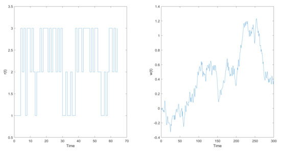
Figure 1. (Left) Setting the number of steps equal 64, we have a three states Markov chain stair figure. (Right) Setting the number of steps equal 300, we have a Brownian motion figure.

In our numerical experiments, we consider two one-dimensional SDEwMS. We choose the sample number $N_{sp}=5000$, where $N_{sp}$ is the number of sample paths. The errors of global weak convergence can be measured by:

$$e_{\mathsf{\Delta }t}^{global}:=|\frac{1}{N_{sp}}{\displaystyle \sum _{i=1}^{N_{sp}}}(\phi \left(X_i^N\right)-\phi \left(X_{i,t_N}\right))|,$$

and the average errors of local weak convergence can be measured by:

$$e_{\mathsf{\Delta }t}^{local}:=|\frac{1}{N_{sp}}\frac{1}{N}{\displaystyle \sum _{i=1}^{N_{sp}}}{\displaystyle \sum _{j=1}^N}(\phi \left(X_i^j\right)-\phi \left(X_{i,t_j}\right))|,$$

where $N=1/\mathsf{\Delta }t$, $\mathsf{\Delta }t$ are $2^{-3},2^{-4},2^{-5},2^{-6},2^{-7}$. We let $\phi \left(X_i^j\right)=sin\left(X_i^j\right)$. Assume $X_i^j$ and $X_{i,t_j}$ are the numerical solution and explicit solutions at the time $t_j$, respectively, where $j\in \{1,2,...,N\}$.

Example 1.

We consider the Ornstein–Uhlenbeck (O-U) process for SDEwMS:

$$\left\{\begin{array}{c}d{X}_t=-X_{t}f\left(r_t\right)dt+g\left(r_t\right)d{W}_t,\hfill \\ X_0=1.5,r_0=1,\hfill \end{array}\right.$$

(34)

where $W_t$ is a one-dimensional Brownian motion. The Markov chain $r_t$ is in $\mathbb{S}=\{1,2,3\}$ and $W_t$ and $r_t$ are assumed to be independent. The group coefficients f and g are given by

$$f\left(1\right)=1.9,g\left(1\right)=0.04,f\left(2\right)=1.8,g\left(2\right)=-0.03,f\left(3\right)=1.7,g\left(3\right)=0.02.$$

It is well known that Equation (34) has the explicit solution

$$X_t=X_0{e}^{{\int }_0^t-f\left(r_s\right)ds}+{\int }_0^t{e}^{-f\left(r_s\right)(t-s)}g\left(r_s\right)d{W}_s.$$

In Table 1, we set the time $t\in [0,1]$, where the terminal time is $T=1$. CR stands for the convergence rate with respect to time step $\mathsf{\Delta }t$. We compute global errors and average local errors (Avg.local errors) of the new scheme. We can get that global convergence rate (Glo.CR) and average local convergence rate (Avg.local CR) have the order 2.0 and order 3.0, respectively. For more intuitive display, we show the numerical results of the local and global errors in Figure 2 (left). In Table 2, we simply utilize the Euler scheme and Runge–Kutta scheme to make a comparative experiment with the new scheme. It is easily to know that the new scheme has the most precision, but it also takes longer CPU time than Runge–Kutta scheme. For more intuitive display, the CPU Time and result of errors of all schemes are shown in Figure 2 (right). In addition, Figure 3 shows the mean-square stability of the new scheme with three kinds of time steps.

Example 2. 

We consider the following geometrical model for SDEwMS:

$$\left\{\begin{array}{c}d{X}_t=X_{t}f\left(r_t\right)dt+X_{t}g\left(r_t\right)d{W}_t,\hfill \\ X_0=0.1,r_0=1,\hfill \end{array}\right.$$

(35)

where $W_t$ is a one-dimensional Brownian motion. The Markov chain $r_t$ is in $\mathbb{S}=\{1,2\}$ and $W_t$ and $r_t$ are assumed to be independent. The coefficients f and g are given by $f\left(1\right)=1.72,$ $g\left(1\right)=0.35, f\left(2\right)=1.6, g\left(2\right)=0.2.$ It is well known that Equation (35) has the explicit solution

$$X_t=X_{0}exp({\int }_0^t[f\left(r_s\right)-\frac{1}{2}{g}^2\left(r_s\right)]ds+{\int }_0^{t}g\left(r_s\right)d{W}_s).$$

Table 1. Errors and convergence rate of Scheme 1 with the parameters of $f\left(1\right)=1.9,$ $g\left(1\right)=0.04,$ $f\left(2\right)=1.8, g\left(2\right)=-0.03, f\left(3\right)=1.7, g\left(3\right)=0.02$ in Example 1.

N	Global Errors	CR	Avg.local Errors	CR
8	5.069 × ${10}^{-3}$		1.895 × ${10}^{-3}$
16	1.288 × ${10}^{-3}$	1.9768	2.455 × ${10}^{-4}$	2.9484
32	2.891 × ${10}^{-4}$	2.0659	2.979 × ${10}^{-5}$	2.9955
64	6.942 × ${10}^{-5}$	2.0726	4.207 × ${10}^{-6}$	2.9487
128	1.789 × ${10}^{-5}$	2.0491	6.006 × ${10}^{-7}$	2.9113

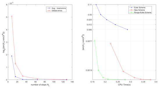
Figure 2. (Left) The global error and Avg.local error of Scheme 1 for Example 1. (Right) The correlations for global errors and CPU Time of all schemes.

Table 2. Errors and convergence rates of all schemes with the parameters of $X_0=5,$ $f\left(1\right)=1.65,$ $g\left(1\right)=0.05,$ $f\left(2\right)=1.8,$ $g\left(2\right)=0.02$.

N	8	16	32	64	128	CR	CPU Time(s)
Euler Scheme	1.128 × ${10}^{-1}$	5.250 × ${10}^{-2}$	2.534 × ${10}^{-2}$	1.249 × ${10}^{-2}$	6.201 × ${10}^{-3}$	1.0174	1.078436
New Scheme	7.221 × ${10}^{-3}$	1.656 × ${10}^{-3}$	4.207 × ${10}^{-4}$	1.022 × ${10}^{-4}$	2.471 × ${10}^{-5}$	2.0428	1.525335
Runge–Kutta Scheme	7.789 × ${10}^{-3}$	1.858 × ${10}^{-3}$	4.503 × ${10}^{-4}$	1.186 × ${10}^{-4}$	2.799 × ${10}^{-5}$	2.0241	1.011832

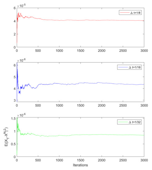
Figure 3. Mean–square stability of three kinds of time steps of global errors with New Scheme.

In Table 3, we find that Example 2 can also obtain that Glo.CR and Avg.local CR have the order 2.0 and order 3.0 of the new scheme. In Figure 4 (left), we clearly show that the global errors are different between a single state and switching states. In Table 4, for all three schemes, we fix a rational upper bounds of state values and find that the convergence rate of the new scheme will tend to order 1.0 when all state values become bigger. Meanwhile, the convergence rates of Milstein scheme and Euler scheme stay stable at order 1.0. In Table 5, for all three schemes, we fix the state difference and find that the convergence rate of the new scheme decline rapidly when all state values become bigger. The convergence rate of the new scheme is even negative when the state values are extremely big. Meanwhile, the convergence rates of Milstein scheme and Euler scheme are very low when the state values are extremely big. For more intuitive display, Figure 4 (right) shows the change process of convergence rate with the change times of state values (CTSV).

Table 3. Errors and convergence rate of Scheme 1 with the parameters of $X_0=0.1,$ $f\left(1\right)=1.72,$ $g\left(1\right)=0.35, f\left(2\right)=1.6, g\left(2\right)=0.2$ in Example 2.

N	Global Errors	CR	Avg. Local Errors	CR
8	4.688$\times {10}^{-3}$		2.153$\times {10}^{-4}$
16	1.173$\times {10}^{-3}$	1.9981	2.600$\times {10}^{-5}$	3.0496
32	3.006$\times {10}^{-4}$	1.9813	3.314$\times {10}^{-6}$	3.0108
64	7.413$\times {10}^{-5}$	1.9913	3.904$\times {10}^{-7}$	3.0293
128	1.811$\times {10}^{-5}$	2.0016	5.099$\times {10}^{-8}$	3.0145

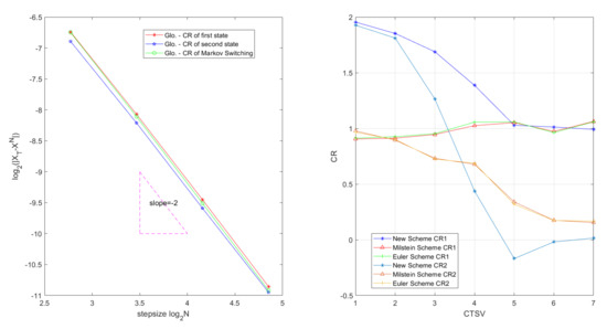
Figure 4. (Left) The convergence rates of different states. (Right) The variations in two methods of state values and the variations in the convergence rates of three schemes.

Table 4. Multiple groups of state values and convergence rates of three schemes with $X_0=0.25$.

$\left[f\left(1\right),f\left(2\right)\right]$	$\left[3,2.8\right]$	$\left[3,2.4\right]$	$\left[3,1.8\right]$	$\left[3,1\right]$	$\left[3,0.1\right]$	$\left[3,0.02\right]$	$\left[3,0.01\right]$
$\left[g\left(1\right),g\left(2\right)\right]$	$\left[0.35,0.3\right]$	$\left[0.35,0.25\right]$	$\left[0.35,0.2\right]$	$\left[0.35,0.15\right]$	$\left[0.35,0.1\right]$	$\left[0.35,0.05\right]$	$\left[0.35,0.01\right]$
New Scheme CR1	1.9545	1.8527	1.6883	1.3866	1.0283	1.0126	0.9912
Milstein Scheme CR1	0.9052	0.9125	0.9456	1.0253	1.0523	0.9726	1.0626
Euler Scheme CR1	0.9125	0.9254	0.9522	1.0565	1.0583	0.9626	1.0596

Table 5. Multiple groups of state values and convergence rates of three schemes with $X_0=0.25$.

$\left[f\left(1\right),f\left(2\right)\right]$	$\left[2,1.5\right]$	$\left[3.5,3\right]$	$\left[5.5,5\right]$	$\left[8,7.5\right]$	$\left[12.5,12\right]$	$\left[15,14.5\right]$	$\left[17.5,17\right]$
$\left[g\left(1\right),g\left(2\right)\right]$	$\left[0.3,0.2\right]$	$\left[0.4,0.3\right]$	$\left[0.6,0.5\right]$	$\left[1,0.9\right]$	$\left[1.8,1.7\right]$	$\left[2.8,2.7\right]$	$\left[3.5,3.4\right]$
New Scheme CR2	1.9265	1.8109	1.2638	0.4379	−0.1687	−0.0187	0.0149
Milstein Scheme CR2	0.9771	0.8952	0.7312	0.6779	0.3401	0.1749	0.1549
Euler Scheme CR2	0.9644	0.9012	0.7251	0.6879	0.3182	0.1736	0.1675

5. Conclusions

In this paper, we propose a new weak order 2.0 scheme for solving SDEwMS. By using trapezoidal rule and the integration-by-parts formula, we theoretically prove the new scheme has order 3.0 convergence under local weak condition. Two numerical experiments are given to confirm theoretical results. In addition, the first numerical experiment is also given to compare the New Scheme with other schemes, such as Euler scheme and Runge–Kutta scheme on convergence rate and accuracy, and the second numerical experiment is also given to explain that the change of Markov chain has some effects on convergence rate of all schemes. According to above experiments, we can obtain that the new scheme has the most precision of all schemes but costs longer time. Moreover, we also find that the maximum state difference and the upper bounds of state values have some effects on all schemes.

References

- Zhou, N.; Mamon, R. An accessible implementation of interest rate models with Markov-switching. Expert Syst. Appl. 2012, 39, 4679–4689. [Google Scholar] [CrossRef]
- Siu, T.; Ching, W.; Fung, E.; Ng, M.; Li, X. A high-order Markov-switching model for risk measurement. Comput. Math. Appl. 2009, 58, 1–10. [Google Scholar] [CrossRef][Green Version]
- He, H.; Qi, W.; Kao, Y. HMM-based adaptive attack-resilient control for Markov jump system and application to an aircraft model. Appl. Math. Comput. 2021, 392, 125668. [Google Scholar]
- Mao, X. Stability of stochastic differential equations with Markovian switching. Stoch. Process. Their Appl. 1999, 79, 45–67. [Google Scholar] [CrossRef]
- Mao, W.; Mao, X. On the approximations of solutions to neutral SDEs with Markovian switching and jumps under non-Lipschitz conditions. Appl. Math. Comput. 2014, 230, 104–119. [Google Scholar] [CrossRef]
- Basak, G.K.; Bisi, A.; Ghosh, M.K. Stability of a random diffusion with linear drift. J. Math. Anal. Appl. 1996, 202, 604–622. [Google Scholar] [CrossRef]
- Ji, Y.; Chizeck, H.J. Controllability, stabilizability and continuous-time Markovian jump linear quadratic control. IEEE Trans. Automat. Control 1990, 35, 777–788. [Google Scholar] [CrossRef]
- Yang, Z.; Yin, G.; Li, H. Stability of numerical methods for jump diffusions and Markovian switching jump diffusions. J. Comput. Appl. Math. 2015, 275, 197–212. [Google Scholar] [CrossRef]
- Ma, H.; Jia, Y. Stability analysis for stochastic differential equations with infinite Markovian switchings. J. Anal. Appl. 2016, 435, 593–605. [Google Scholar] [CrossRef]
- Yuan, C.; Mao, X. Convergence of the Euler-Maruyama method for stochastic differential equations with Markovian switching. Math. Comput. Simul. 2004, 64, 223–235. [Google Scholar] [CrossRef]
- Mao, X.; Yuan, C.; Yin, G. Approximations of Euler-Maruyama type for stochastic differential equations with Markovian switching, under non-Lipschitz conditions. J. Comput. Appl. Math. 2007, 205, 936–948. [Google Scholar] [CrossRef]
- Rathinasamy, A.; Balachandran, K. Mean square stability of semi-implicit Euler method for linear stochastic differential equations with multiple delays and Markovian switching. Appl. Math. Comput. 2008, 206, 968–979. [Google Scholar] [CrossRef]
- Zhou, S.; Wu, F. Convergence of numerical solutions to neutral stochastic delay differential equations with Markovian switching. J. Comput. Appl. Math. 2009, 229, 85–96. [Google Scholar] [CrossRef]
- Yin, B.; Ma, Z. Convergence of the semi-implicit Euler method for neutral stochastic delay differential equations with phase semi-Markovian switching. Appl. Math. Model. 2011, 35, 2094–2109. [Google Scholar] [CrossRef]
- Li, R.H.; Chang, Z. Convergence of numerical solution to stochastic delay differential equation with poisson jump and Markovian switching. Appl. Math. Comput. 2007, 184, 451–463. [Google Scholar]
- Chen, Y.; Xiao, A.; Wang, W. Numerical solutions of SDEs with Markovian switching and jumps under non-Lipschitz conditions. J. Comput. Appl. Math. 2019, 360, 41–54. [Google Scholar] [CrossRef]
- Fan, Z.; Jia, Y. Convergence of numerical solutions to stochastic differential equations with Markovian switching. Appl. Math. Comput. 2017, 315, 176–187. [Google Scholar] [CrossRef]
- Nguyen, S.; Hoang, T.; Nguyen, D.; Yin, G. Milstein-type procedures for numerical solutions of stochastic differential equations with markovian switching. SIAM J. Numer. Anal. 2017, 55, 953–979. [Google Scholar] [CrossRef]
- Kumar, C.; Kumar, T.; Wang, W. On explicit tamed Milstein-type scheme for stochastic differential equation with Markovian switching. J. Comput. Appl. Math. 2020, 377, 112917. [Google Scholar] [CrossRef]
- Zhao, J.; Yi, Y.; Xu, Y. Strong convergence of explicit schemes for highly nonlinear stochastic differential equations with Markovian switching. Appl. Math. Comput. 2021, 393, 125959. [Google Scholar]
- Buckwar, E.; Riedler, M.G. Runge-Kutta methods for jump-diffusion differential equations. J. Comput. Appl. Math. 2011, 236, 1155–1182. [Google Scholar] [CrossRef]
- Liu, X.; Li, C. Weak approximations and extrapolations of stochastic differential equations with jumps. SIAM J. Numer. Anal. 2000, 37, 1747–1767. [Google Scholar] [CrossRef]
- Li, Y.; Wang, Y.; Feng, T.; Xin, Y. A New Simplified Weak Second-order Scheme for Solving Stochastic Differential Equations With Jumps. Mathematics 2021, 9, 224. [Google Scholar] [CrossRef]
- Platen, E.; Bruti-Liberati, N. Numerical Solutions of Stochastic Differential Equations with Jump in Finance; Springer: Berlin/Heidelberg, Germany, 2010; Volume 64. [Google Scholar]
- Øksendal, G.; Proske, F. Malliavin Calculus for Lévy Processes with Applications to Finance; Springer: Berlin/Heidelberg, Germany, 2009. [Google Scholar]
Publisher’s Note: MDPI stays neutral with regard to jurisdictional claims in published maps and institutional affiliations. |
© 2021 by the authors. Licensee MDPI, Basel, Switzerland. This article is an open access article distributed under the terms and conditions of the Creative Commons Attribution (CC BY) license (http://creativecommons.org/licenses/by/4.0/).