ConvGraph: Community Detection of Homogeneous Relationships in Weighted Graphs

Abstract

This paper proposes a new method, ConvGraph, to detect communities in highly cohesive and isolated weighted graphs, where the sum of the weights is significantly higher inside than outside the communities. The method starts by transforming the original graph into a line graph to apply a convolution, a common technique in the computer vision field. Although this technique was originally conceived to detect the optimum edge in images, it is used here to detect the optimum edges in communities identified by their weights rather than by their topology. The method includes a final refinement step applied to communities with a high vertex density that could not be detected in the first phase. The proposed algorithm was tested on a series of highly cohesive and isolated synthetic graphs and on a real-world export graph, performing well in both cases.

1. Introduction

Graph theory dates back to when Euler solved Seven Bridges of Königsberg problem in 1736 [1]. Since then, a great deal of progress has been made with respect to knowledge of graphs and their properties, where computers can be used to represent many real networks using these types of models. These real networks are characterized by a high level of order and organization; many low-degree vertices coexist with high or very high-degree vertices, and edges are distributed not only globally but also locally, with high concentrations within special groups of vertices and low concentrations between these groups. These are so-called communities [2].

These communities are, in short, groups of vertices that share properties and play a similar role in the graph but are differentiated from the others. Nowadays, they represent one of the most interesting research lines in social network analysis due to their application in many areas such as biology or sociology, through medicine, to information technologies.

The problem of community detection is not new, and there have been many attempts at solving the problem in different ways in many knowledge areas over time. The first analysis of communities was by Rice in 1927. His research detects communities within small political bodies based on the similarity of their voting patterns [3]. Two decades later, Homans proved that particular social groups could emerge by swapping the rows and columns of particular matrices describing social links to get a block matrix [4]. In 1955, Weiss and Jacobson focused on looking for working groups within a particular state agency. They used a method that established the basis for some of the modern community detection algorithms by eliminating members working with people from different groups, who acted as connectors between groups [5].

Afterwards, it was discovered that a hierarchical structure can emerge in the network, that is, there may be different levels of vertex groups where small communities form part of larger communities. The first approach proposed to detect these vertex groups was data clustering methods [6], specifically hierarchical data clustering methods which are divided into two types: agglomerative methods and divisive methods [7]. Agglomerative methods start from individual vertices which are joined if they are similar enough. Algorithms within this category include single linkage clustering or average linkage clustering.

Divisive methods start from communities that are iteratively divided by removing edges that connect dissimilar vertices. Another approach within clustering methods, partitional methods, where the number of communities, k, is pre-assigned and the data points are embedded in a metric space so that each vertex is a point, and a distance measure between each pair of points in the space is defined. The aim is to separate points into k communities by optimizing a cost function based on the distance between points and/or from points to community centroids. The best-known partitioning method is the k-means clustering method [8].

Another group of clustering methods are the so-called spectral methods, based on decomposing the data into groups by exploiting the algebraic properties of the data matrices. Spectral clustering consists of transforming the initial data into a set of points whose coordinates are elements of eigenvectors, which are then grouped using agglomerative or partitional techniques.

A group of algorithms that warrant special mention are the methods for detecting communities by optimizing some type of cost function, specifically, the modularity function [9], a field in which considerable progress has been made over recent years. The idea is as follows. A random graph is not expected to have community structure. Therefore, the possible existence of communities emerges by comparing the edge density in a subgraph with the expected density if the vertices were added according to a community structure. Thus, the higher the value of the modularity function, the more modular the graph being evaluated is. Obviously, a possible option for ascertaining the optimal community distribution in terms of modularity is to perform an exhaustive search. However, this approach is impossible for a medium-size graph due to the number of possible combinations. Thus, alternative techniques should be used to reach satisfactory, albeit not optimal, solutions.

The first modularity optimization approach was Newman’s greedy algorithm [10], a hierarchical agglomerative clustering algorithm where groups of vertices are successively joined together forming larger and larger communities while modularity increases after each join.

Later approaches were proposed using metaheuristics to avoid the local optima problem. In a first approach by Guimerà et al. [11], simulated annealing was successfully used to optimize modularity using only two types of movements: a local movement, where any of the randomly selected vertices are swapped from one community to another, and a global movement that consists of combining and splitting communities. Another successful metaheuristic used for modularity optimization are genetic algorithms, where partitions are the chromosomes, and modularity is the fitness function as the approach proposed in Tasgin et al. [12].

Duch and Arenas proposed the use of extremal optimization [13] to solve the problem, where the modularity function is rewritten as a sum over the vertices, later defining the local fitness function for each vertex as the ratio between the local modularity of the vertex and the degree of that vertex.

Almost all the methods explained above have two important drawbacks: (1) all the vertices of the graph must belong to a community and/or (2) a number of communities, k, must be given a priori, which is impossible since, in most real cases, the complete visualization of the network is out of the question or contributes nothing, ruling out the definition of k.

There is a class of relatively new techniques that avoid these two shortcomings: density-based community detection methods. These algorithms evolved from density-based clustering methods, such as DBSCAN [14] or DENCLUE [15]. Clusters are defined in DBSCAN as areas with high density of points surrounded by other areas with a low density of points. As a result, points do not necessarily belong to any cluster, and, therefore, DBSCAN is a non-partitional method capable of handling outliers (or noise). The main problem with algorithms like DBSCAN is that they cannot detect overlapping clusters. However, improvements such as OPTICS [16] or HICS [17] have been proposed to solve this problem.

Based on these methods, Huang et al. proposed DenShrink [18], a community detection and parameter-free algorithm that optimizes modularity and identifies hierarchical embedded structures with various densities in complex networks. On the other hand, DenGraph [19] and SCAN [20] were proposed as definite adaptations of DBSCAN to the community detection area. Both methods work very similarly, except for the similarity function they use. DenGraph operates on weighted graphs and considers the weight of the edge as the similarity between vertices. On the other hand, SCAN uses a similarity function based on the graph topology, specifically, the similarity between two vertices is correlated to the number of neighbors that they share.

The main drawback of density-based algorithms in a real-world application is that a huge distance matrix must be computed beforehand. Similarly, the resulting communities are not necessarily highly cohesive. Therefore, many communities could emerge that are, in fact, relatively isolated from the other vertices but are uninteresting according to our search criterion.

We have so far looked at unweighted topology-based community detection methods that, intuitively, they detect communities with a high density of edges within the community itself but are somewhat isolated from the remainder. However, most of the real-world applications are applied to weighted graphs, that is, graphs with weights assigned to their edges. The algorithms described above are not very useful, if not useless, for these types of graphs, because they cannot be easily adapted.

Along these lines, Liu et al. proposed the ABCD algorithm [21], which detects communities in large complex weighted networks based on the definition of attraction of a community. Jaho et al. also proposed the ISCoDe algorithm [22], where the weights of the edges are computed according to vertex similarity, outputting user groups with similar interests.

In this paper, we propose the ConvGraph method, a new community detection algorithm in weighted graphs incorporating the topological approach, searching for highly cohesive and isolated communities with a high sum of weights with respect to the outside. This approach can be very useful for tax fraud, as it searches for fraud schemes that move a huge amount of money between the companies in the scheme and very little to companies outside the scheme, where there is no justification for the amount moved inside the scheme.

This paper is divided into four sections: Section 2 describes the ConvGraph method, a highly cohesive and isolated community detection algorithm based on edge weights. In Section 3, we check the performance of the ConvGraph method on a series of highly cohesive and isolated synthetic graphs and a real-world exportation graph. Finally, some conclusions are outlined in Section 4.

2. ConvGraph: A Weight-Based Method for Detecting Highly Cohesive and Isolated Communities

The aim of this paper is to propose a novel method to detect highly cohesive and isolated communities in which the value of the sum of the weights of the relationships within the communities is far greater than for the external relationships. For this purpose, we define a transformation of the original graph in a line graph in which each vertex represents a $(u,v)$ relationship of the original graph and each edge in the transformed graph represents the fact that the two relationships in the original graph have at least one vertex in common.

Definition 1.

Let $G=<V,E>$ be a weighted graph where V and E are the vertices and edge sets, respectively. We define a line graph of G as the undirected and weighted graph $H=h_g=<E,R>$, where each vertex $e\in E$ has associated the value $f\left(e\right)\in \mathbb{R}$ of the relationship that it represents in G. Given two vertices $e_1=(u_1,v_1),e_2=(u_2,v_2)\in E$, there will be an edge $r\in R\subseteq \left\{(e,d)\right|(e,d)\in E^2\wedge e\ne d\}$ between them if and only if the relationships that they represent have any vertex of G in common, that is, if $\{u_1,v_1\}\cap \{u_2,v_2\}\ne \varnothing$.

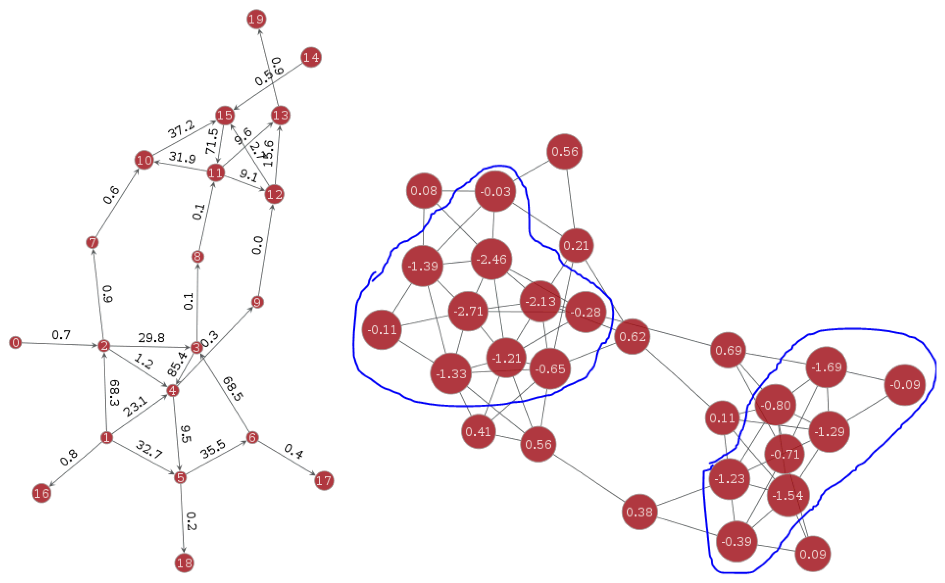
As Figure 1 shows, the edge linking vertices 0 and 1 in the original graph becomes vertex “e0-10” in the line graph. Vertex “e0-10” is linked to the vertices “e1-10”, “e2-1900”, and “e3-2100” with edges whose weights are calculated as the difference in absolute value of the weights of the edges in the original graph, that is, the weights of the edges are $0=10-10$, $1890=1900-10$ and $2090=2100-10$, respectively.

The line graph is used to detect the optimal edges that separate the communities whose relationships have a high weight sum with respect to the remainder of the graph. To do this, we use computer vision methods designed to detect optimal edges in images, as explained in Section 2.1.

2.1. Line Graph Convolution

Let I be an image represented as a set of values in a matrix, where each value corresponds to the pixel intensity, and the adjacency of the pixels is represented by the adjacency of the cells in the matrix. A common concept in computer vision is the image gradient. The image gradient defines the variation of intensity of the pixels in an image through the vector

$$\nabla f=\left[\frac{\partial f}{\partial x},\frac{\partial f}{\partial y}\right].$$

(1)

The direction of this vector f indicates the direction of the image surface in which the intensity $f(x,y)$ increments faster, and therefore pinpoints major intensity changes, see Figure 2.

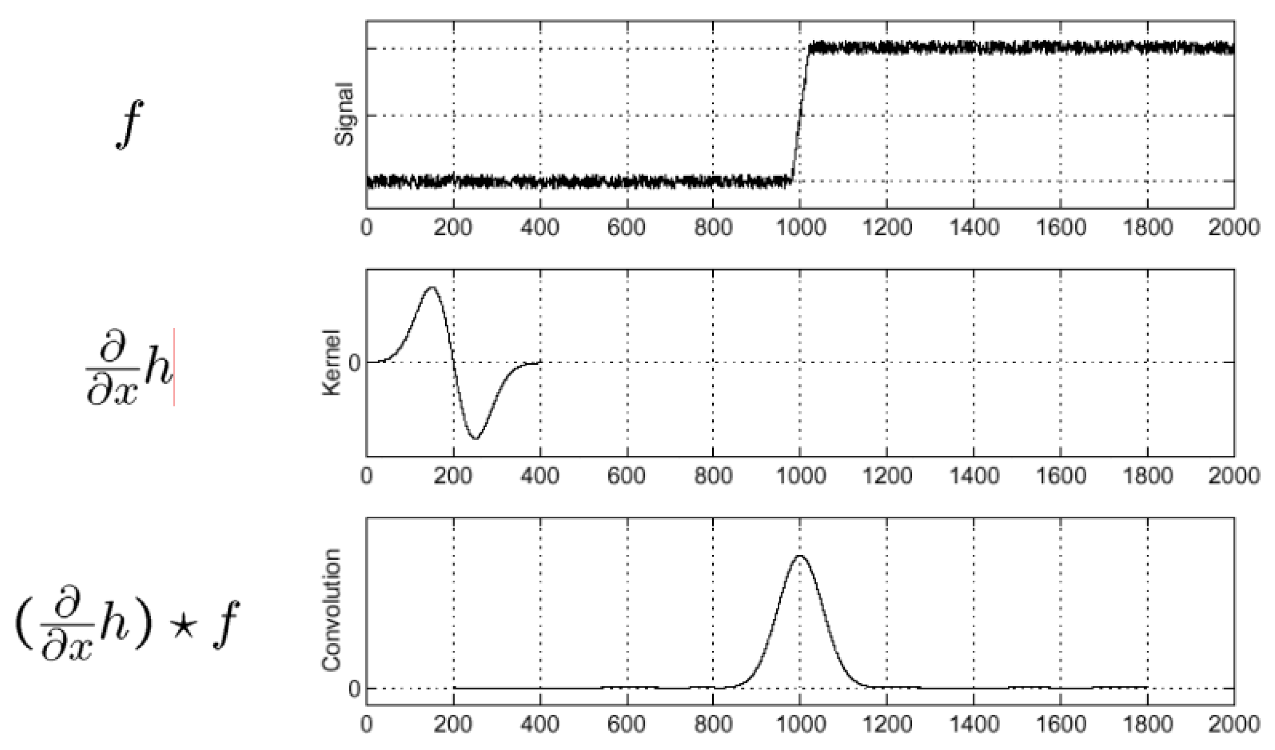
Then, if we are able to detect sudden changes, we can detect an edge, a border between two intensity levels, as we know where the intensity changes are. As a result, we can define regions within the image and detect communities with pixels of similar intensities. However, it does not always suffice to compute the image gradient. When the image has a lot of noise in an area, the intensity levels move around constants with a radical change in intensity. As a result, we get a white noise signal as a gradient, that is, a normal distribution signal with constant variance and zero mean.

Figure 3 shows the intensity of a one-dimensional image with a sudden change in intensity at its center but with noise at both levels. If we compute the derivative using Equation (1) to get the gradient vector of the image, we find in Figure 4 that it is around zero. However, there are big changes due to the noise of the signal, which makes it impossible to distinguish the intensity border. In other words, the derivative of the signal fluctuates around zero because the two intensities of which it is composed each oscillate around a constant with a lot of noise, and there is a very pronounced jump between the two.

One way to solve this problem is to apply a smoothing filter to the image, or kernel, using a Gaussian function. The basic idea is to take the intensity of each pixel and combine it with the intensity values of adjacent pixels. In other words, we take the intensity value and its neighbors, which we add by multiplying each of them by the weights that follow a Gaussian distribution, attaching less importance to furthest pixels. This averages intensity values and smoothes the noise. This operation is called convolution.

Definition 2.

Let h and f be two functions, and the convolution operation (*) is defined as

$$(h\ast f)\left(x\right)={\int }_{-\infty }^{\infty }h(x-t)f\left(t\right)dt$$

(2)

As in the computer vision application, the proposed algorithm works in the finite and discrete environment of each pixel, using the following adaptation

$$(h\ast f)\left(x\right)=\sum _{t=-S}^{S}h(x-t)f\left(t\right),$$

(3)

for a given size $S\in \mathbb{Z}$.

Therefore, when we apply the convolution f with the Gaussian function h, the new intensity of each pixel x is computed attaching more weight to x and less to the pixels in its neighborhood $E\left(x\right)$ that are further away from x, thus smoothing intensity, as shown in Figure 5 ($h\ast f$). By deriving this result, a peak forms at the point where there is a big change in the initial signal intensity, see Figure 5 ($\frac{\partial }{\partial x}(h\ast f)$).

Since the convolution operation is commutative, this process can be reduced to a single operation since

$$\frac{\partial }{\partial x}(h\ast f)=\left(\frac{\partial }{\partial x}h\right)\ast f.$$

(4)

To prove that the above equality is true, remember Definition 2 explaining the convolution operation. Assuming a continuous and differentiable h, we can apply Leibniz’s rule to derive under the integral sign [23], whereby we demonstrate the equality of Equation (4)

$$\begin{array}{c}\hfill \frac{\partial }{\partial x}(h\ast f)=\frac{\partial }{\partial x}{\int }_{-\infty }^{\infty }h(x-t)f\left(t\right)dt=\\ \hfill {\int }_{-\infty }^{\infty }\frac{\partial }{\partial x}h(x-t)f\left(t\right)dt={\int }_{-\infty }^{\infty }\frac{\partial h(x-t)}{\partial x}f\left(t\right)dt=\\ \hfill \left(\frac{\partial }{\partial x}h\right)\ast f.\end{array}$$

(5)

Hence, we can apply the kernel derivative directly as shown in Figure 6.

The problem would then be reduced to finding peaks once the convolution is computed. However, it may be difficult to define what a peak is. Therefore, instead of a kernel created from a Gaussian function, we can use the Laplacian of Gaussian (the second derivative of the Gaussian function), which will denote the changes in intensity as a change of sign, see Figure 7.

Since an image can be represented as a graph of adjacent pixels, the problem of finding homogeneous communities in weighted graphs after applying the transformation discussed above to output the line graph is equivalent to finding changes between intensity regions in images, taking into account the following equivalencies: image ≡ graph; pixel ≡ vertex; pixel intensity ≡ vertex weight; and pixel adjacency by matrix position ≡ adjacency of vertices by edges. With these equivalencies, we can define Algorithm 1 to detect communities in weighted graphs.

Figure 8 shows an illustrative example of the ConvGraph Algorithm (Algorithm 1).

Algorithm 1: ConvGraph: Community detection of homogeneous relationships in weighted graphs.

Data: $G=<V,E>$ weighted graph and $\frac{{\partial }^2}{\partial x^2}h$ Laplacian kernel

Result: communities detected by the convolution of the weighted graph

—Transform the weighted graph G into its line graph H;

—Apply the kernel $\frac{{\partial }^2}{\partial x^2}h$ with a convolution on the graph H;

—Where there is a change of sign, we have the edge of two communities;

—Use a ratio that measures the internal weights of the community with respect to the total weights of the graph to select the community if the value is significantly high;

—Pinpoint on the original graph the vertices that lie on the edges represented by the vertices of the line graph for the detected communities;

2.2. Deriving High-Density Communities

Once Algorithm 1 has been applied, communities are identified by their weights rather than by their topology deriving good results if parameters are correctly fixed in the Laplacian kernel. However, Algorithm 1 does not correctly identify all the vertices in very dense communities. To avoid this problem, a second filtering is performed for high-density communities with a high density level to identify the other irrelevant vertices as independent communities or as one large community.

In order to measure the density of a graph $G=<V,E>$, we use the clustering coefficient, which is expressed as

$$c_i=\frac{|e_{jk}|}{k_i(k_i-1)}:v_j,v_k\in N_i,e_{jk}\in E,$$

(6)

where $c_i$ is the clustering coefficient for vertex i, $k_i$ is the outgoing degree of vertex i, and $N_i=v_j:e_{ij}\in E$ is the subset of vertices with edges whose origin is i and the target is j. The clustering coefficient of G, $C_i$, can be computed as the average of all the $c_i$. This coefficient quantifies the clustering of vertex $v_i$ with values in the range $[0,1]$, where the value will be higher the more the cluster resembles that of a clique that is adjacent to all the vertices of the graph. We can consider graphs with $C_i\ge 0.7$ as being highly dense.

The second filtering process to be performed for high-density communities is shown in Algorithm 2.

Algorithm 2: Deriving high-density communities.

Data: Weighted graph $G=<V,E>$ and set of communities C Result: Set of expanded communities S    —For each community $t\in C$, compute its density $D\left(G_t\right)$;    —If $D\left(G_t\right)>threshold$, then Algorithm 1 is applied to the community subgraph, $G_t$, and its neighbors;    —If any neighbor is identified with the same subgraph $G_t$, it is added to t;

3. Results

The algorithm was developed entirely in Python and tested on an HP (HP, 1-21, Camí de Can Graells, 08174, Sant Cugat del Vallès, Barcelona, Spain) Pavilion G6 with 8 GB of RAM and an Intel i5 CPU at 2400 MHz.

3.1. Results with Synthetic Graphs

In this section, we evaluate the quality of communities detected by the proposed algorithm by generating some synthetic graphs containing highly cohesive and isolated communities (with a higher edge density inside than outside the communities). Later, a small sample of 150 of these graphs with minor variations are also be analyzed, and the results are evaluated.

To do this, a function generating random graphs containing highly cohesive and isolated communities has been created from the triplet $(T,E,D)$, with $T=[a_1,a_2,..a_n]$, where $a_i$ is the number of vertices of the community, i, and E is the number of extra vertices that will be added to the graph once the communities defined by T have been generated, and D is the approximate density of the resulting graph. To ensure the random behavior of the function, both the number of vertices and the edges will be generated from a normal distribution $\mathcal{N}(E,E/4)$. Since isolated vertices are not relevant to the problem, they are removed from the graph to focus only on the connected component.

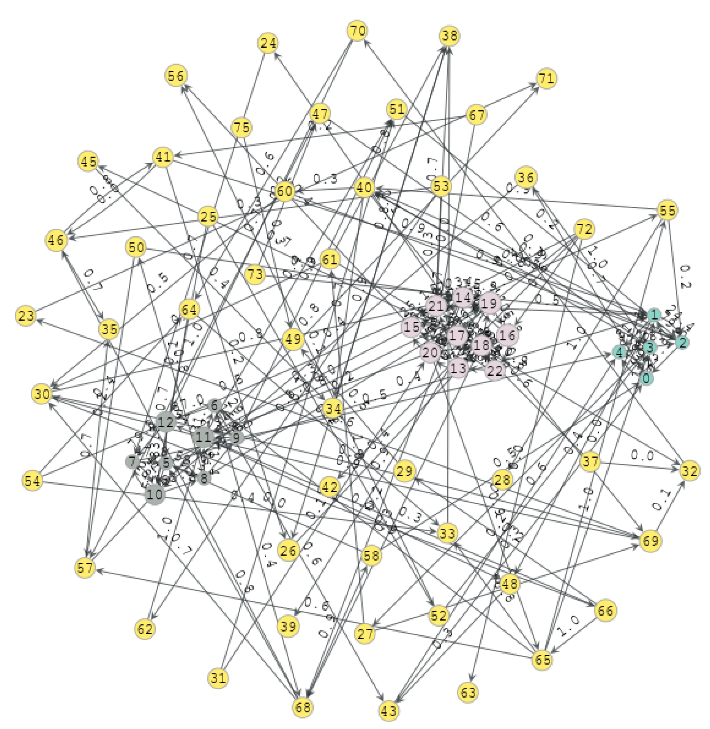
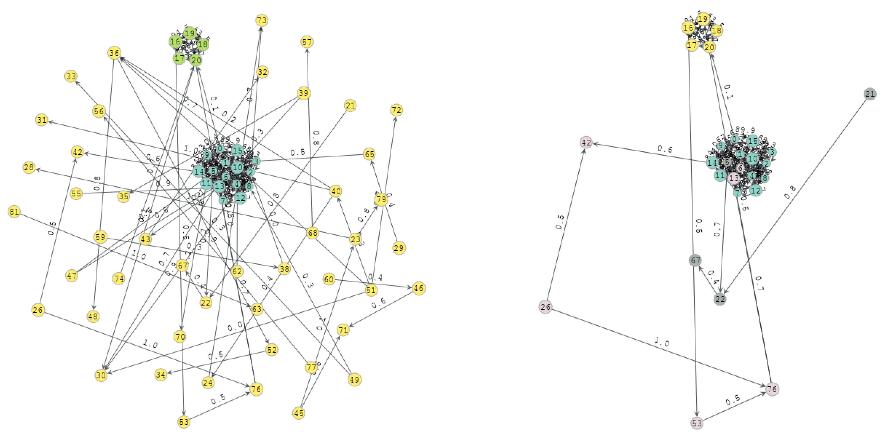
The graph shown in Figure 9 was generated with a total of 73 vertices, 172 edges, and a real density of 0.033, where the three communities of 5, 8, and 10 vertices are highlighted in blue, gray, and pink, respectively, and the extra vertices are shaded yellow. The yellow vertices are detected as a separate community. Thus, once the convolution and filtering procedure is applied, it is possible to evaluate the detection process carried out by the algorithm.

On the other hand, an evaluation function has also been created. This function returns a quality score by comparing the communities detected by the proposed algorithm with the communities previously generated by our random graph generator function. The score is based on three fundamental aspects: a community vertex detection success rate, a penalty if the algorithm fails to isolate communities and, obviously, the number of detected communities.

The score can be expressed as follows:

$$score=\frac{{\sum }_{i=0}^n{p}_i^{\ast }}{n+1}\times 100-\left|\right|M|-(n+2)|,$$

(7)

where M is the set of different labels assigned to the graph, $n+2$ is the number of communities in a perfect classification ($n+1$ highly cohesive initial communities and one additional community with the extra vertices), and $p_i^{\ast }$ is the hit ratio having applied the penalty for bad isolation.

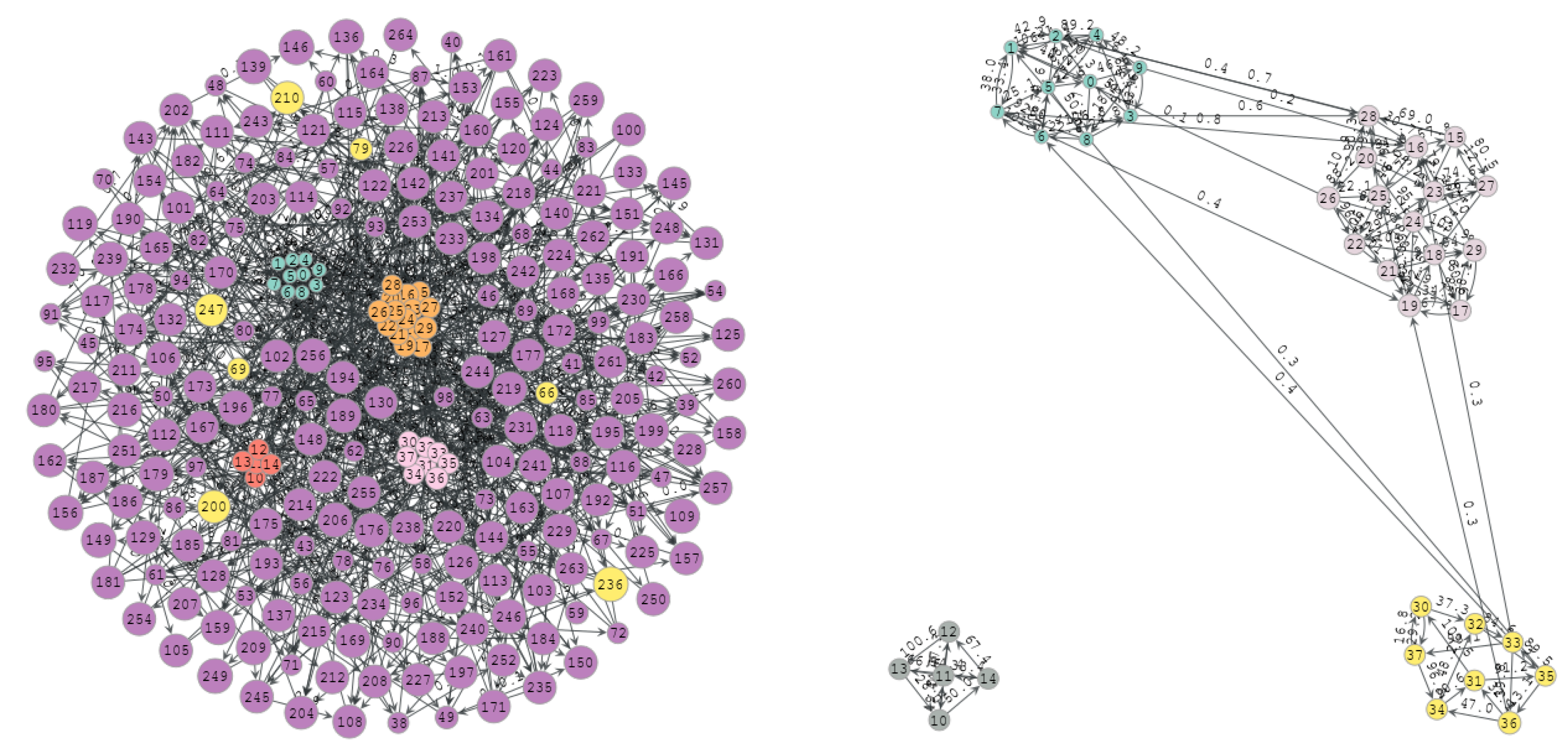
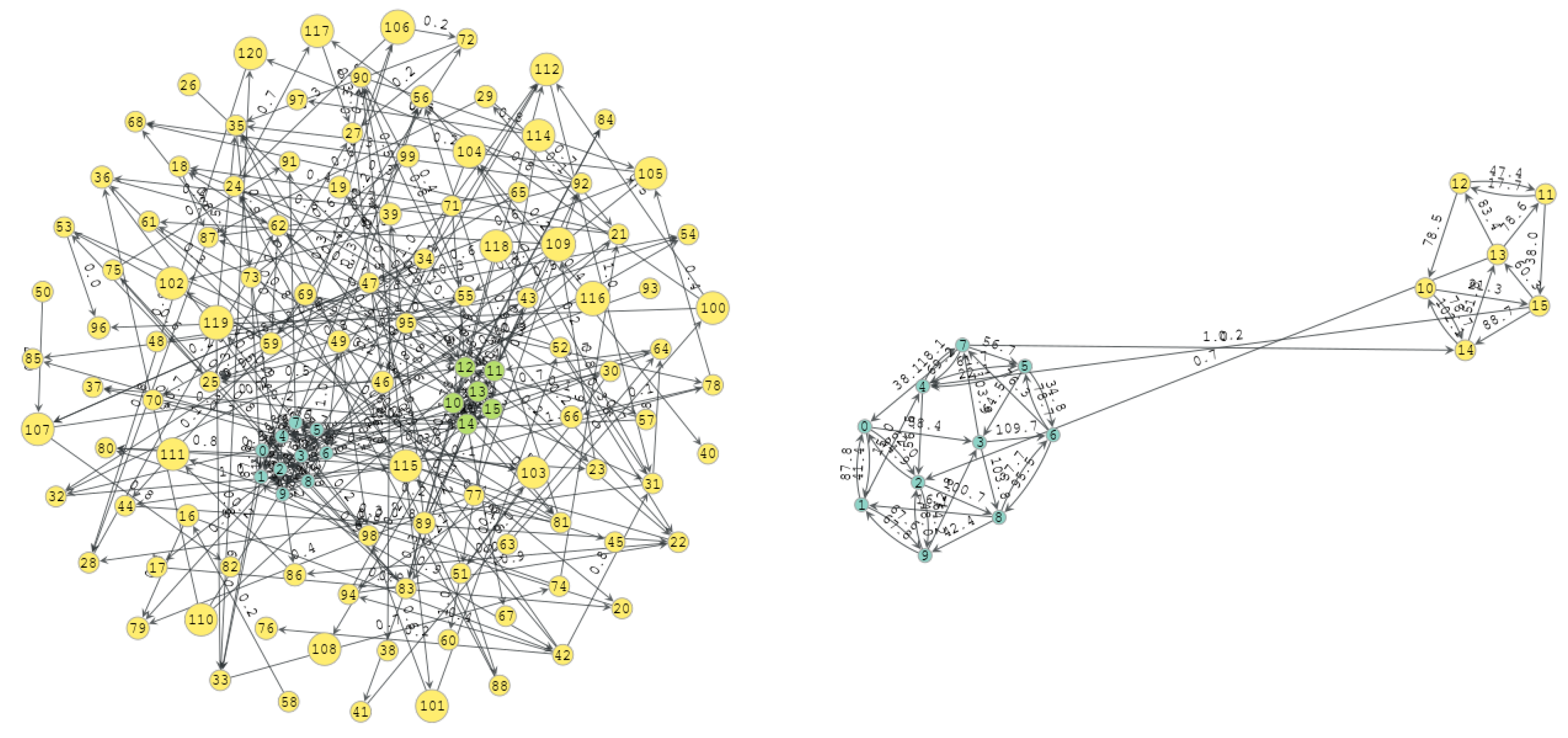
We start by applying our algorithm to a graph with a lot of noise, that is, with small communities and many extra vertices so that the algorithm will have to differentiate the noise from the communities of interest. Then, we generate a graph according to the following parameters $T=[10,5,15,8]$, $E=200$, and $D=0.01$. The generated graph is shown in Figure 10. There are four communities of interest (blue, brown, green, and pink), each with 10, 5, 15, and 8 vertices and 200 extra vertices. Figure 10 includes a total of 263 vertices and 795 edges with a real density of 0.0115. The number of extra vertices is some units of magnitude greater than the number of vertices within the communities of interest. Therefore, the algorithm has to be able to separate the noise from the really interesting communities.

Figure 11 shows the results derived after applying Algorithm 1.

Hit ratio $TA=[1.0,0.8,0.93,1.0]$ indicates the hit ratio for each community, that is, how many of the original vertices are part of the detected community. We find that the rate for each of the communities detected by the algorithm is greater than 80%.

These hit ratios are improved by applying the second filtering process based on Algorithm 2 to $HR=[1.0,1.0,1.0,1.0]$, correctly detecting all communities and their vertices (Figure 12). Of the global score, 99% is due to the detection of an additional community that was not in the original graph (vertices highlighted in yellow).

The results of applying the proposed method to different graphs of various sizes and densities are discussed below.

The graph in Figure 13 was generated using parameters $T=[10,6]$, $E=248$ and $D=0.0174$. It has a total of 264 vertices and 120 edges, with two communities of 10 and 6 vertices, respectively. As shown in Figure 13, the two original communities were detected with a hit ratio of $HR=[1,0,1.0]$ and a global score of 98%, since another two communities were detected but not identified as highly cohesive.

The graph in Figure 14 was generated with parameters $T=\left[16\right]$, $E=648$ and $D=0.005$. It consists of 664 vertices and 335 edges, with a single community with 16 vertices. The original community was detected with a hit ratio of $HR=\left[1.0\right]$ and a global score of 99% due to the detection of an additional community.

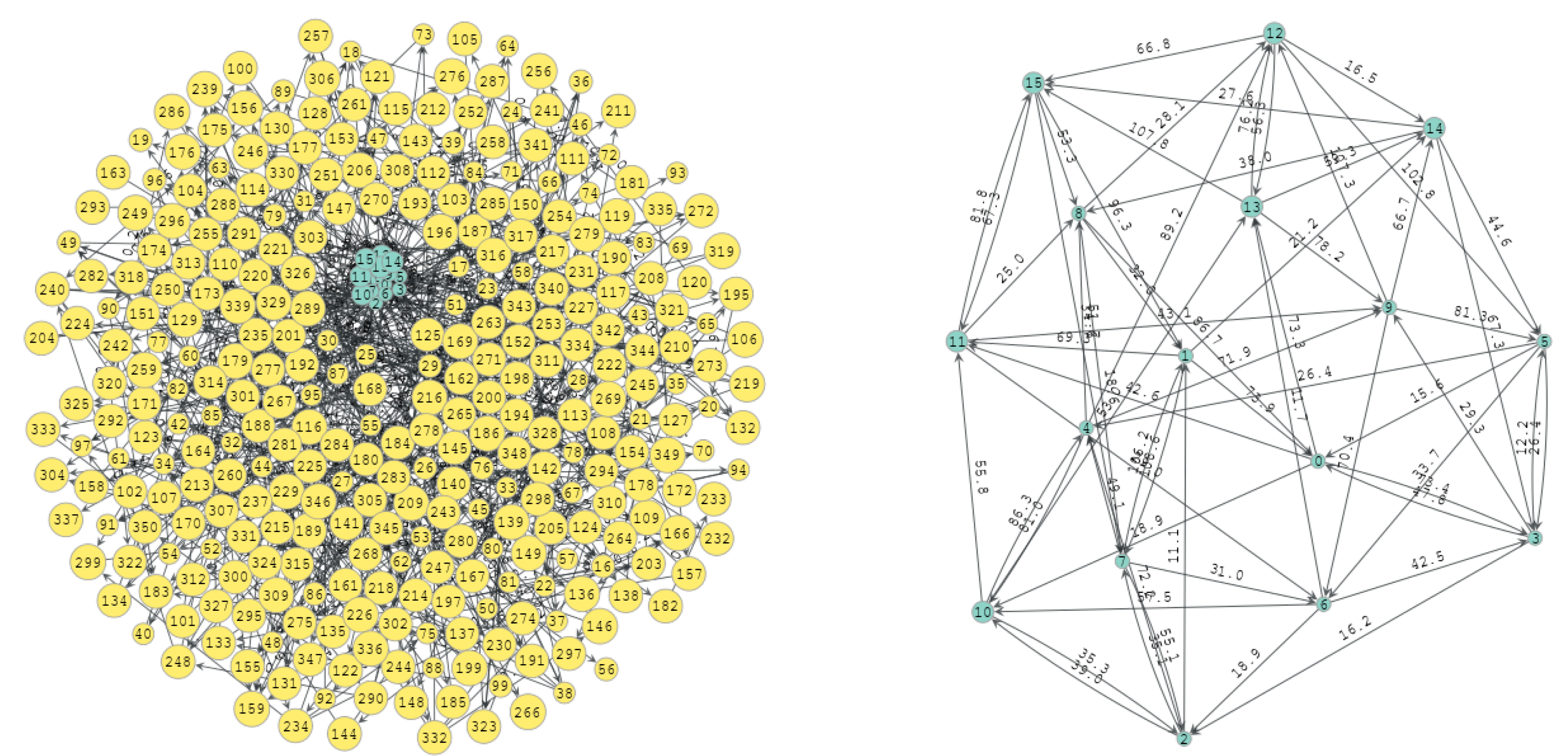
The graph in Figure 15 was generated with parameters $T=[16,5]$, $E=126$ and $D=0.028$, with a total of 147 vertices and 67 edges. The detection rate with a hit ratio of $HR=[0.813,1.0]$ was good but not perfect. As a result, one of the communities was not completely detected, and the global score was reduced to 56.16%. At any rate, even though the wrongly detected community did not exactly match the original community, the detection rate was over 80% of the hit ratio. Therefore, the detection rate can be considered to be good.

The graph in Figure 16 was generated with parameters $T=[16,5,8,22]$, $E=27201$ and $D=0.012$ with a total of 27,242 vertices and 1460 edges. This graph is hard to detect properly since there is a lot of noise introduced by the difference in units of magnitude between the number of vertices of each community with respect to the total number of graph vertices. Even so, the hit ratio is more than acceptable at $HR=[0.94,0.8,1.0,0.73]$. However, as Figure 16 shows, only three of the original four communities are detected as relevant. Therefore, the vertices of the fourth community were mixed in with the extra vertices. Moreover, another two communities were also detected. On these grounds, the global score dropped to 48.32%.

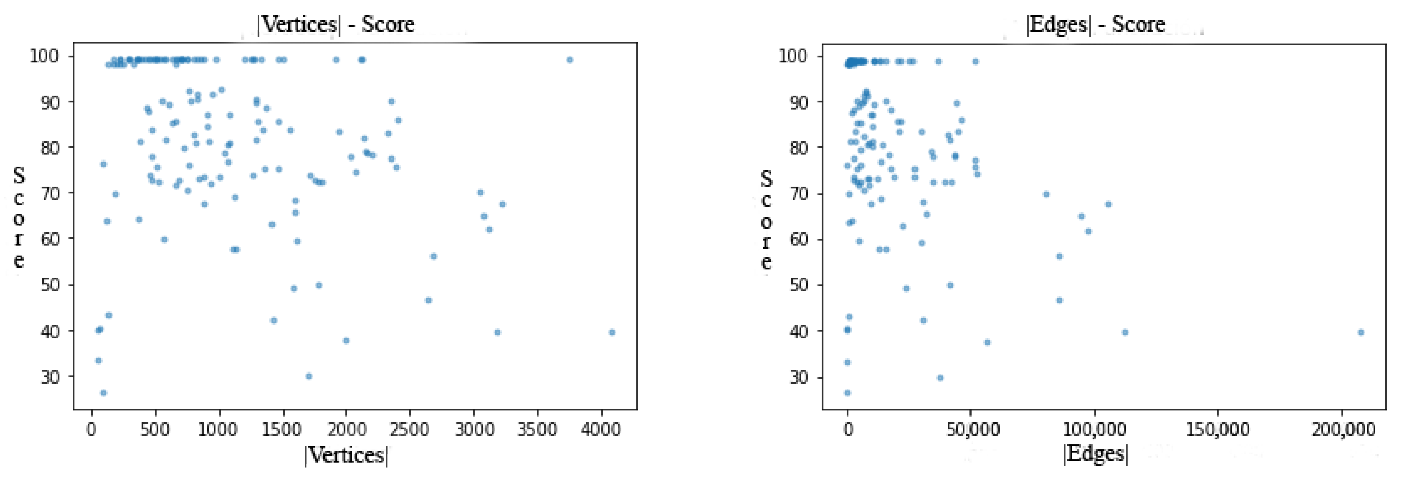
Looking at the figures above, we realize that the greater the number of vertices, the more difficult it is to properly visualize the original graph with its communities. Therefore, we carried out a small descriptive analysis on a sample of 150 graphs with a total number of vertices and edges impossible to visualize and a number of communities ranging from 2 to 10, with up to 25 vertices per community and a fixed reference edge density of 0.01.

Figure 17 show that most of the sample graph communities are detected properly, as they get good or very good global scores. Note that, as expected, the greater the number of vertices and edges, the more difficult it is for the proposed method to achieve a good detection rate due to the noise that is introduced. In this sense, it is found to be much more sensitive to a high edge density than to a vertex degree. Nonetheless, the method is stable up to 3500 vertices and 50,000 edges, much stabler than most of the already known community detection techniques.

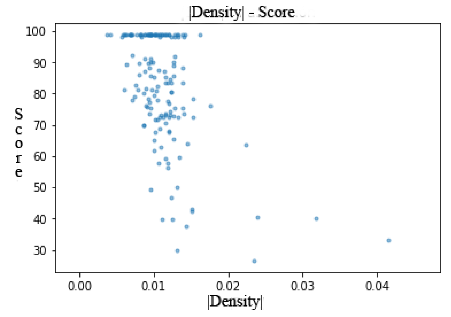
Figure 17 shows that the number of edges detracts from the detection rate more than by the degree of the graph. Thus, as the number of edges is what most contributes to increasing graph density, we can deduce that a high density contributes to poor detection. This is evident from Figure 18, showing the ratio between the density of the sample graphs and their global score. We find that the detection rate of the ConvGraph method drops as density increases.

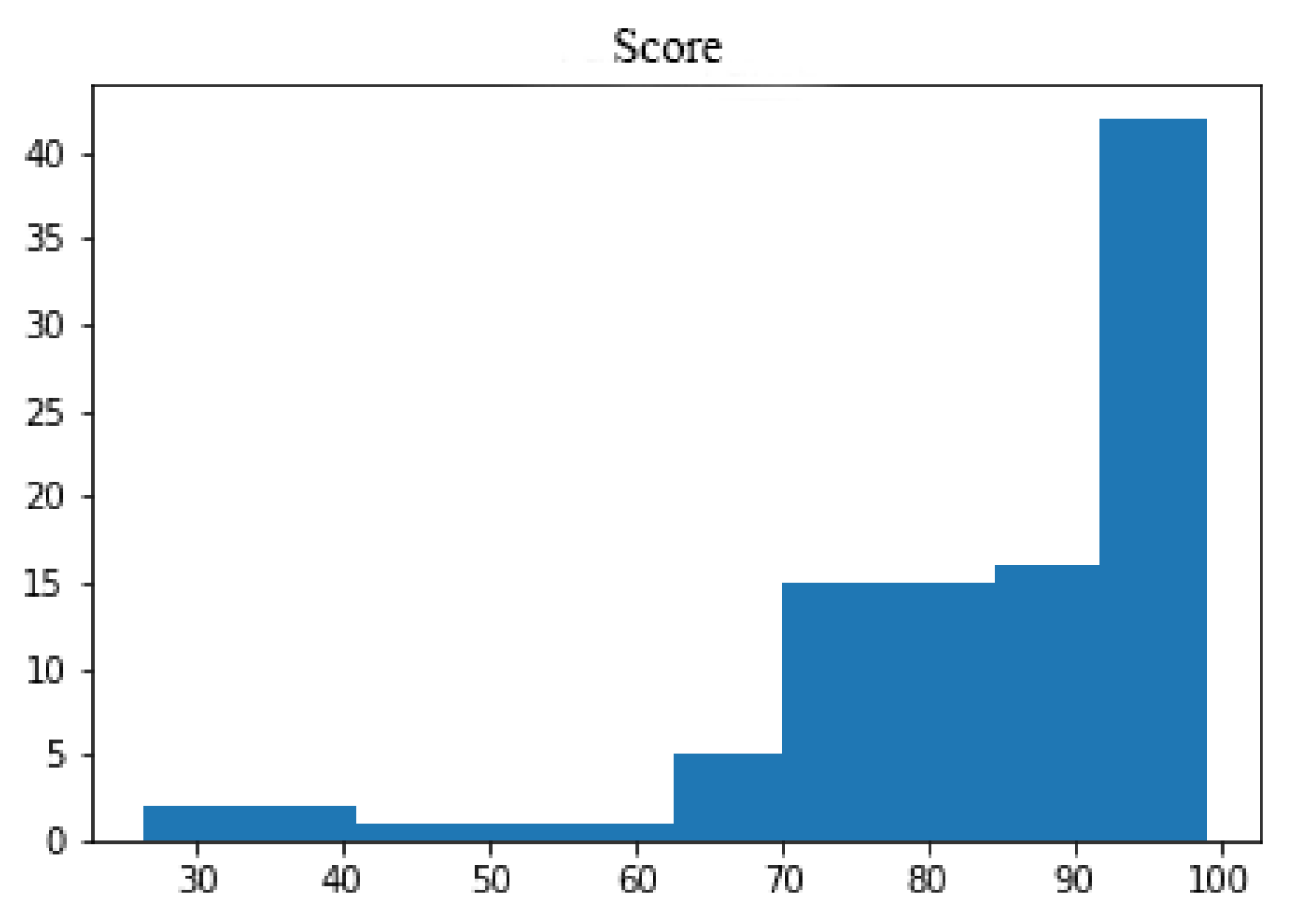
Despite this, the ConvGraph method performs very well for the randomly generated graphs in the sample, as demonstrated in the histogram shown in Figure 19. Scores range from 70% to 100%, with most falling within 90% to 100%. Thus, we can conclude that the ConvGraph method operates stably even in graphs with medium or high noise.

3.2. A Real-World Case

In Section 3.1, we tested the performance of the ConvGraph method on synthetic graphs. In this section, the method is applied to a real-world graph. For this purpose, we use the world export network 1997–2014 available at http://microdata.worldbank.org/index.php/catalog/2545/data-dictionary/F31?filename=CYD_all (accessed on 20 January 2021), providing a series of 73 variables relating to exports, plus the year and the countries of origin and destination.

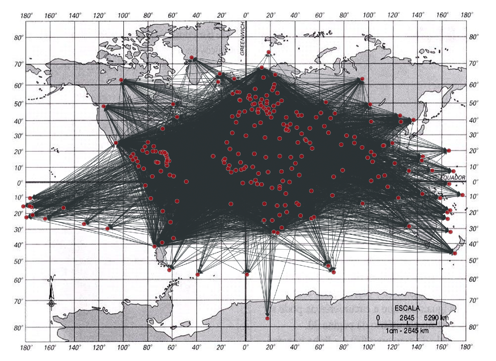
However, this example considers the number of exports for the year of study between the countries of origin and destination only. After removing the remaining variables, we grouped the number of exports by origin and destination to compute the sum of the exports for all years between each pair of vertices, thus removing the parallel edges. After removing the parallel edges, the graph was generated from the resulting file, including 251 vertices corresponding to each of the related countries and 12,049 edges corresponding to each of the export relations between the countries (see Figure 20).

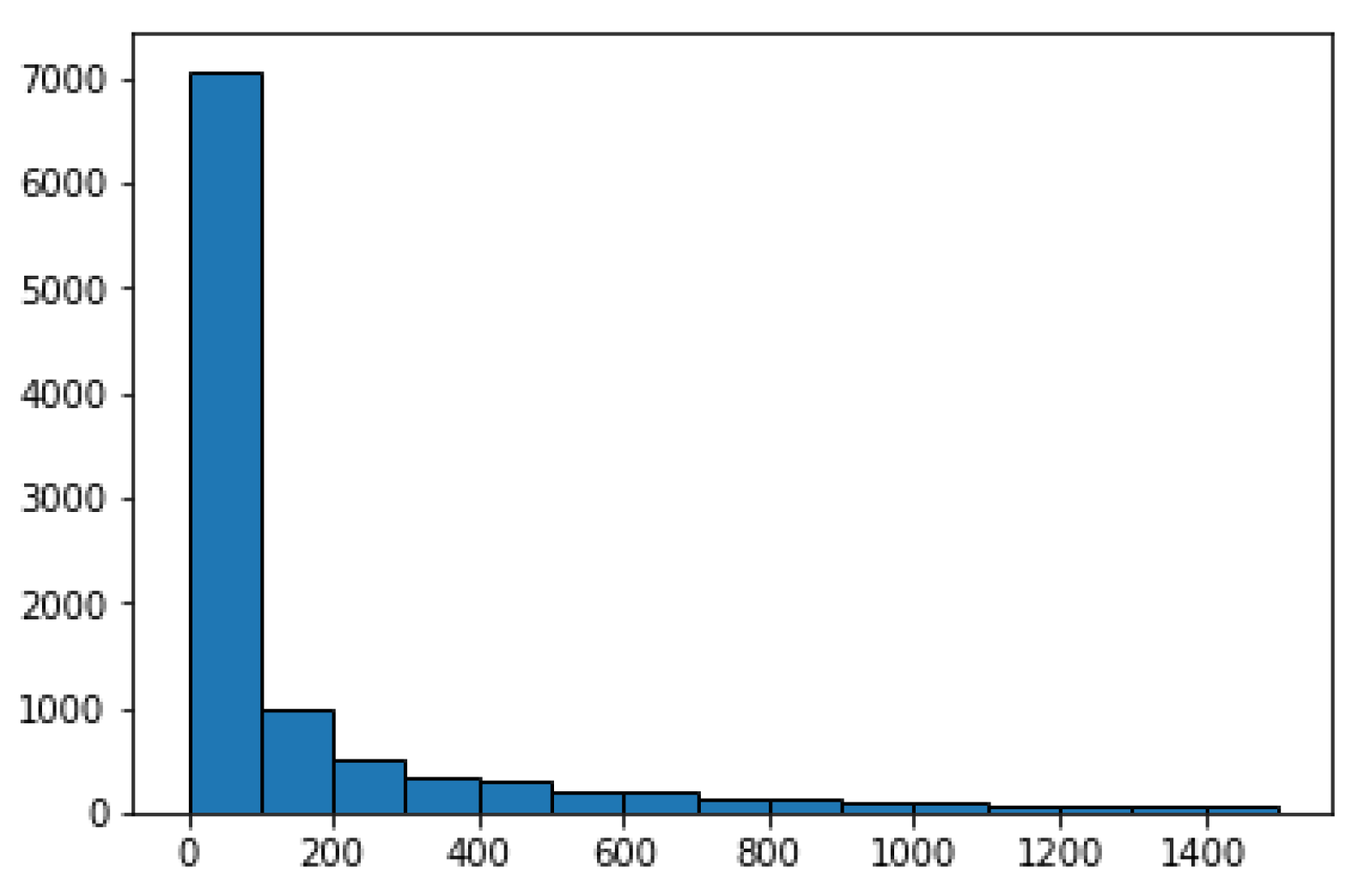
The only assumption made by the ConvGraph method is that some weights in the graph should be considerably higher than others. In our real-world graph, this assumption should hold since countries with strong export policies should have much higher weights than countries where exports do not really play a significant role in their economies. The respective histogram shown in Figure 21 demonstrates that the assumption does indeed hold. There are edges with very low weights (approximately 67% with fewer than 200 exports), whereas the others range from 200 to 339,338 exports.

The ConvGraph method has two parameters, corresponding to the size and standard deviation of the kernel used in the convolution that have to be fixed for the graph under consideration to achieve its best performance. For efficiency reasons, the size of the filter was fixed at 5 since, in the different tests carried out with the synthetic graphs, it output good performance. Computation time grew with larger filter sizes. Regarding standard deviation, values $i=0.2,0.22,0.24,0.26,...,0.78,0.80$ were tested in the first phase of the ConvGraph method. Better quality communities were detected in the graph with a value of $0.8$, which was established as the standard deviation, i.e., $K(5,0.8)$.

The communities detected in the execution are listed below:

The algorithm took 40 min to detect the communities in

Table 1. Results of applying ConvGraph on the export graph.

Community ID	Latitude	Country
Community 1	Central America	Venezuela, Colombia,
		Ecuador
Community 2	Central America	Nicaragua, Costa Rica,
		Panamá
Community 3	America	Argentina, Brazil,
		Chile, Guatemala,
		Honduras, Mexico,
		Paraguay, El Salvador
		Uruguay, USA
Community 4	Nordic countries and Russia	Denmark, Estonia,
		Finland, Faroe Islands,
		Lithuania, Latvia,
		Norway, Russia,
		Sweden
Community 5	Western Europe and Africa	Angola, Andorra,
		Cape Verde, France
		Morocco, Portugal,
		Spain
Community 6	Central Asia	Armenia, Georgia,
		Azerbaijan
Community 7	Central Europe	Croatia,
		Bosnia-Herzegovina,
		Macedonia, Serbia,
		Slovenia
Community 8	Africa	Kenya, Rwanda,
		Sudan, Tanzania
		Uganda
Community 9	Africa	South Africa, Mozambique,
		Zambia, Zimbawe
Community 10	Africa	Reunion, Mauritius Islands
		Seychelless
Community 11	Intercontinental	Germany, Haiti,
		United Arab Emirates,
		Switzerland, Iran,
		Dominican Rep., Iraq,
		Pakistan

. This is quite a good running time considering the complexity of the graph. The export communities are quite logical since they are communities formed by countries that are geographically close to each other, since most countries export to nearby countries on the grounds of costs and customs. A case apart is Community 11 focused on fuel export relations, formed by countries from four continents. Therefore, we can conclude that the ConvGraph method performs well with not only synthetic but also real-world graphs.

4. Conclusions

This paper proposes a novel method, the ConvGraph method, for detecting highly cohesive and isolated communities in weighted graphs, where the sum of the weights is significantly higher inside than outside the communities. To do this, we apply a filter, based on a convolution process as applied to detect edges in computer vision.

The performance analysis carried out on both synthetic graphs and a real-world export graph shows that the ConvGraph method is quite robust to noise, since the detection rate does not drop much if the ratio of the number of vertices to be detected to the total number of vertices in the graph is small. On the other hand, it is rather sensitive to graph density, like most community detection techniques.

One issue requiring improvement is the dependence on the kernel parameters. It has been proven, for example, that odd kernel size values yield better results than even sizes in the graphs used. This is because taking only half a function of the Laplacian is in the odd sizes in which it takes a first value close to the minimum of the function (negative), in the case of an even value, that first value is already close to zero and is significantly far from that minimum value because the function grows fast. For now, the size has been adjusted to a value of 5 and a standard deviation of between 0.7 and 0.9 for which the ConvGraph method performed best. It would be very interesting to render the technique independent of any parameter and enrich the method with an algorithm that automatically adjusts these parameters.

Another future research line is the application of the ConvGraph method to tax fraud and money laundering as a result of close collaboration with the National Fraud Investigation Office attached to the Spanish Ministry of Finance.