Abstract
At the end of 2019, an outbreak of the novel coronavirus (COVID-19) made a profound impact on the country’s production and people’s daily lives. Up until now, COVID-19 has not been fully controlled all over the world. Based on the clinical research progress of infectious diseases, combined with epidemiological theories and possible disease control measures, this paper establishes a Susceptible Infected Recovered (SIR) model that meets the characteristics of the transmission of the new coronavirus, using the least square estimation (LSE) method to estimate the model parameters. The simulation results show that quarantine and containment measures as well as vaccine and drug development measures can control the spread of the epidemic effectively. As can be seen from the prediction results of the model, the simulation results of the epidemic development of the whole country and Nanjing are in agreement with the real situation of the epidemic, and the number of confirmed cases is close to the real value. At the same time, the model’s prediction of the prevention effect and control measures have shed new light on epidemic prevention and control.
1. Introduction
The coronavirus (CoV) derives its name from the fact that the virus with typical glycoprotein resembles a crown or solar corona under electron microscope. Coronaviruses are single-stranded RNA viruses and contain the largest known RNA genomes, ranging from 27 to 32 kilobases in length [1]. They belong to the family Coronaviridae, order Nidovirales, and widely exist in nature. Apart from human beings, the coronavirus has a wide range of hosts. It can be isolated from various animals such as camels, pigs, cattle, chickens, ducks, geese, cats, dogs, mice, and bats, which may cause an infection in the respiratory system, digestive system, and nervous systems [2,3].
Since it was first identified and described in 1965, three major large-scale outbreaks have occurred, namely the Severe Acute Respiratory Syndrome (SARS) in 2003, the Middle East Respiratory Syndrome (MERS) in 2012, and MERS in 2015 [4].
On 12 December 2019, the Wuhan Health Commission confirmed 27 cases of pneumonia caused by unacquainted virus [5], and the number of infections gradually increased. On 7 January 2020, Chinese authorities confirmed a novel coronavirus as the pathogen source of the pandemic [6]. On 1 February 2020, the World Health Organization (WHO) declared the novel coronavirus (COVID-19) as a Public Health Emergency of International Concern (PHEIC) [7]. On 11 February 2020, at the Global Research and Innovation Forum opened in Geneva, WHO Director-General Ghebreyesus announced at a press conference that the new coronavirus was named “COVID-19”. Since the outbreak, the WHO has maintained close communication with the Chinese government in several aspects, including the identification and treatment of infected individuals, follow up monitoring of novel coronavirus pneumonia close contacts, and the publicization of pandemic prevention and control policies.
As of 31 January 2020, the total number of coronavirus cases around 23 provinces in China (including Hong Kong, Macao, and Taiwan) as well as Thailand, Japan, Malaysia, Germany, the United States, Australia, and so on, reached 11,955, with 234 deaths [8]. The speed of spread of infectious diseases is often measured by the basic regeneration number of the virus. In this pandemic, since the probability of the outbreak and the time of peak occurrence under different interventions are not clear yet, further research is needed.
On 20 January 2020, the National Health Commission of China (NHC) included novel coronavirus pneumonia in the class B infectious diseases stipulated in the Law of the People’s Republic of China on the Prevention and Control of Infectious Diseases, and carried out prevention and control measures in accordance with the class A infectious diseases. Under the norms of laws and policies, some pandemic intervention measures have been gradually implemented, such as gathering virus infected persons to designated places for separate isolation and treatment, medical isolation and observation of close contacts, close observation of personnel in the pandemic focus, etc. The effectiveness and impact of these measures on pandemic control need to be quantitatively studied. The research in this area has important practical significance for formulating appropriate pandemic prevention and control measures after the outbreak in other areas.
The start of the pandemic occurred during the Spring Festival travel rush in Wuhan, the largest land and water transportation hub of China’s mainland, which has a huge scale of population flow. According to data released by Wuhan municipal, from the start of the pandemic to the lockdown, there were about five million residents who left Wuhan. Therefore, on 23 January 2020, Chinese authorities enacted lockdown in seven cities in Hubei, including Wuhan, Ezhou, Huanggang, Chibi, Xiantao, Zhijiang, and Qianjiang, which effectively caused the travel restriction of more than 40 million people. In order to slow down the spread of the pandemic, and avoid the pandemic breaking out in other regions, the Chinese government invested resources and paid a high price in these measures to reduce the spread of the virus to other regions. However, how much effect these measures can play in the prevention and control of the pandemic is currently unknown.
Following the impact of the novel coronavirus on the general population, estimating the natural growth of the virus can determine the probability and the peak time of the outbreak, so as to provide the basis for policymakers to formulate and implement reasonable and effective interventions. This allows pandemic interventions to better protect the general population and control the pandemic on the premise of minimum impact on social–economic development and people’s livelihoods.
Many scholars have been studying the spread of infectious diseases for a long time, which can date back to 1760, when D. Bernoulli [9] proposed a mathematical model of the transmission of variola. In recent years, mathematical research on infectious diseases has made rapid progress. In 1998, Shulgin and Stone [10] introduced seasonal variation based on the Susceptible Infected Recovered (SIR) model, and created a deterministic model under the same rate of birth and death. Lekone [11] and others created the Susceptible Infected Exposed Recovered (SEIR) model for Ebola virus transmission in 2006. In 2016, Talawar [12] used the MCMC method to estimate the SIR model parameters by taking into account that recovery and infection times are continuous. Using the Markov Chain Monte Carlo (MCMC) method, Talawar estimated the SIR model parameters by considering the continuity of recovery and infection time. Later, scholars around the globe conducted additional research on infectious diseases. For instance, Florea and Lzureanu (2020) simulated the spread of infectious diseases by using the Susceptible Infected Susceptible Model (SIS) system [13]; Zhang et al. (2017) studied the spread of infectious diseases in the transportation system [14]. Under the circumstances of a pandemic, it is necessary to conduct research accounting for public health intervention measures. Therefore, our research is of both theoretical and practical significance.
2. Methods
In this chapter, Section 2.1 firstly explains the source of the data and visualizes the change in the pandemic situation by using curve graphs; Section 2.2 introduces the SIR model used in this article in detail; Section 2.3 discusses an LSE method used to estimate parapets in our model; Section 2.4 introduces the calculation method of the basic regeneration number from the perspective of pandemic transmission dynamics.
2.1. Data
The data are from the NHC in China for COVID-19 between 20 January 2020 and 31 January 2020 in China’s mainland. On 3 February 2020, we collected the pandemic-related data published every day from the content column of “pandemic prevention and control dynamics” on the official website of the National Health Commission [15]. It contains total confirmed, recovered, and dead cases (Figure 1). Since the NHC of China adopted a daily reporting system for the pandemic, we sorted the above-mentioned data in units of days, and carried out research using the same unit of time.
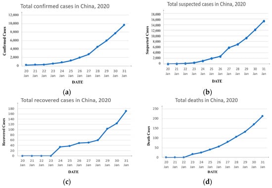
Figure 1.
Official statistics. (a) The number of confirmed cases due to COVID-19 from 20 January to 31 January; (b) the number of suspected cases due to COVID-19 from 20 January to 31 January; (c) the number of recovered cases due to COVID-19 from 20 January to 31 January; (d) the number of deaths due to COVID-19 from 20 January to 31 January.
2.2. The Model
In this paper, we proposed a pandemic model based on the SIR model associated with the progress of clinical research, epidemiological development, and different interventions. We used the Chinese mainland’s novel coronavirus pneumonia cases from 20 January 2020 to 31 January 2020 to estimate the model parameters and calculate the basic reproduction number of the new coronavirus disease in China. We then analyzed the effectiveness of interventions such as quarantining suspected cases and suspending public transportation, to predict the possibility of a future pandemic outbreak.
The SIR model was proposed by Kermack and Mckendick in 1927 [16]. In this paper, using the core ideas of the SIR model, the population under consideration is divided into three compartments: susceptible (), infective (), and removed (). The susceptible class () represents those individuals who can obtain the disease but are not yet infective. The infective class () refers to those who have been infected with the virus and are transmitting the disease to the susceptible class. The removed class () consists of those who are removed from the susceptible–infective interaction by recovery with immunity, or death.
Based on current research on COVID-19 by experts, for directly transmitted pathogens, the following assumptions are made in our epidemiological models:
- The population considered with constant size is large enough that the fraction of each class can be considered a continuous variable. Since this pandemic occurs rapidly, the model does not include natural births or natural deaths.
- The population is regarded as a homogenous mixture, and the daily contact rate is the average number of effective contacts per infective per day. In other words, is the contact rate times the probability of transmission given a contact between a susceptible and an infectious individual [17,18].
- Individuals are removed from the infective class by recovery at the rate and by death at the rate . Both of them are proportional to the class size with a proportionality constant.
- Despite the opinion of researchers that recovered individuals would still be susceptible to novel coronavirus [19,20], there has been no case of reinfection among recovered people. Thus, in this paper, we assume recovered individuals are conferred with permanent immunity and could not be infected by others again. Then, the rate of transfer from to is .
Thus, our SIR model is appropriate for the situation where individuals recover from COVID-19 with permanent immunity. Under this context, the compartmental diagram for this SIR model is given in Figure 2.
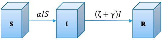
Figure 2.
The compartmental diagram for the SIR model. Flows represent the fractions of the total populations flows from the donor compartments per unit time.
Let , , and be the fractions of the total populations in theses compartment of , and respectively at time . We obtain the following system of differential equations:
We define the initial susceptible population in the SIR model as and the number of infected people as . Moreover, in system (1), it follows that
Since can be replaced by and by using , it is sufficient to analyze the initial value problem in the phase plane.
We define the average number of effective contacts per patient as . This is defined as the number of infectious contacts during the infection period. When the patient has effective contact with a healthy person, the healthy person will become infected and become a patient.
To help analyze the transmission of a novel coronavirus, we define the calculation of the contact σ in the infectious period, which is presented in Equation (2).
For a better understanding of the behaviors of solutions, we try to view their orbits in the phase. Only considering in the equations of system (1), the behaviors of solution paths in the phase are described as
By integrating both sides of Equation (3), we can obtain the following equation:
in which is an integration constant that can be derived from and as:
Since system (4) satisfies
for all , the function remains a constant along with a solution of (3).
Then, phase plane portraits of solution paths are presented below.
The epidemiologically reasonable region in the phase is the triangle given by
The goal of using the phase is to analyze removal rate . A phase portrait corresponding to the solution path (5) is given in Figure 3.
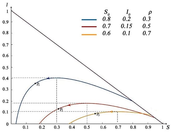
Figure 3.
Phase portrait for the SIR model. Each curve depicts the solution path for different parameter values.
As shown in Figure 3, we define the initial susceptible population in the phase trajectory as and the number of infected people as . The arrows in the figure indicate the changing trends of and as time increases. With the variation in removal rate , the arrival time of the peak value of the curve is different. Additionally, when , it is the highest point of the curve, as shown in , , and points in Figure 3. With , as shown in Figure 3, the corresponding peaks of are . Considering , for instance, if the point of initial values falls on the left side of the vertical line , decreases monotonically to as . That is, the number of patients gradually decreases and disappears eventually. When the initial value of was on the right side of the line , with the increase in , the value of increases, and the number of patients with infectious diseases increases until the passes the point of , at which point begins to decrease gradually and towards to zero.
The arrow direction on the phase trajectory represents the time process of the continuous spread of the disease after the occurrence of the disease. It can be found that under different intervention price adjustments, the number of infected people will eventually be cleared up as time goes by, that is, the disease will eventually be effectively controlled.
The corresponding parameter values of each phase trajectory curve are listed in Table 1.

Table 1.
Parameter values of each phase track.
From the above discussion on the change in the phase trajectory, the following conclusions can be drawn:
(1) If , then decreases to zero as , which represents that the infectious individuals will disappear quickly;
(2) If , then the number of infectious individuals first increases up to a maximum value , and then decreases to zero as . That is, the virus will spread for some time but eventually die out.
In conclusion, it is possible to control infectious diseases in two aspects, namely by reducing the susceptible individuals and increasing the relative removal rate .
2.3. Least Squares Method for Parameters Estimation
Accurate estimation of parameters is the basis for the precise prediction of infectious diseases. The traditional least square estimation (LSE) method generally finds the optimal solution of the parameter estimates by solving the minimum Sum of Squared Errors (SSE) [21]. In the SIR model, the basic idea of the least square method is to minimize the sum of the squared error between the number of infective persons in the fitting model and the actual number of infective persons.
During the spread of infectious diseases, the confirmed cases and daily new cases are known, while the number of susceptible patients is difficult to identify, so it can be regarded as an unknown parameter. Infectious rate , recovery rate , and death rate are essential unknown parameters in the novel coronavirus SIR model. Here, we use the LSE method to estimate the parameters of our model.
In the model, we define that the unknown parameter . We use to represent the number of people in each part of the SIR model, . The actual observed value of the infective class is denoted by , and the model simulation value of infective people is . The corresponding errors is expressed as . Then, the SSE of can be written as:
The goal is to obtain an estimated value of the unknown parameter and find the minimum . By calculating the derivative of Equation (6) about , we get:
Let Equation (7) be equal to zero, and then the LSE of the parameters , and can be obtained by Matlab. In this paper, the collected pandemic data are substituted into Equation (7) for simulation verification. The simulation results can be seen in Section 3.
2.4. Pandemic Spreading Dynamics Analyses
In addition to estimating the parameters of our SIR model, we are also concerned with . In this paper, refers to the number of second-generation cases that can be infected under ideal conditions [22]. When a case enters the susceptible population, the larger the number of , the more difficult it is to control the pandemic without any intervention [23]. That is, tells us about the rate of spread of the disease. Under normal circumstances, is the threshold of the occurrence of the pandemic, which can be expressed as follows.
If , then a pandemic will not occur, while if , an initial case will lead to an outbreak, so the disease will take and infect the entire population in the area eventually [24].
Let , and is a subset of the hyperplane . For the novel coronavirus SIR model in this paper, the process of deriving its basic reproductive ratio is shown in Figure 4 [25]. In Figure 4, is the transmission time of infectious diseases, and implies the total number of people in the area involved.
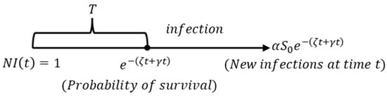
Figure 4.
The evolution of infective individuals, where is the disease-free equilibrium in the feasible region .
As given in Figure 4, represents the time period of disease transmission. It can be seen that in an environment where all the people are susceptible, a coronavirus infective individual who was infected at time has the probability that they will remain infectious for at least time . Thus, the number of newly infected individuals is at time . Then, we obtain [26]:
3. Real Data Applications
Current studies show that COVID-19 is a new pathogen, so people of all ages are immune to new coronavirus and are generally susceptible to infection [27]. For this pandemic, the official notification of the epicenter was the Huanan Seafood Market in Wuhan [28]. The local hospital reported the first unexplained pneumonia case on 8 December 2019, which was diagnosed as having been infected by a novel coronavirus. During the 40 days from 8 December 2019 to 19 January 2020, there was a giant flow of population in the market for the Lunar New Year, and these people were scattered in all regions of Wuhan, and the virus can infect all kinds of people. Therefore, we set the population of Wuhan as the initial susceptible population, that is, the value of S (0) is 12.3 million. We define the susceptible population of the initial state nationwide as the number of people with initial diagnosis nationwide as , and the number of rehabilitation and death cases in the initial state nationwide as Taking 20 January 2020 as the initial state nationwide, there is , , .
3.1. Prediction Results Based on COVID-19 SIR Model
With the development of the pandemic, China’s NHC has generated statistics on asymptomatic infections and confirmed cases separately. Because asymptomatic infections do not have clinical symptoms after diagnosis, such as fever, cough, and sore throat, it can take a period of time for some asymptomatic infections to become diagnosed. Therefore, the NHC makes it clear that asymptomatic infections are not confirmed cases and are not new infected patients. Therefore, asymptomatic infections are not included in the confirmed case data in this paper [29].
On the one hand, very few cases of asymptomatic infections have been reported. On the other hand, the diagnosis of these cases is often delayed. This paper believes that asymptomatic infections can be counted as confirmed cases only after official diagnosis.
Predicted from the model, the reproductive ratio of COVID-19 is estimated to be 6.47, and other estimated parameters are shown in Table 2.
Table 2.
COVID-19 model parameter estimation of China.
With the above parameter estimations, the infection trend of COVID-19 can be predicted. Through model calculation, we convert the percentage calculated in the model into the number of different types of people. According to our model, in the context of current interventions (before 31 January 2020), the nationwide estimated infections as a function of time would increase to a peak after 25 days, that is, around 14 February 2020. In reality, the second round of outbreaks peaked in mid-to-late February, with little difference between model predictions and reality. At the same time, Wuhan saw zero new confirmed cases for several consecutive days in the middle of March 2020. If calculated according to the date of 20 March 2020, the time interval from the first outbreak report on 8 December 2019 was 102 days, indicating that the prediction of the model is relatively accurate.
Figure 5 shows the development process of the COVID-19 pneumonia starting point from 20 January 2020 to 100 days. We can see that up to 45,737 people were infected at the peak of this pandemic. From the overall forecast of the pandemic, we can find that the pandemic would gradually disappear after 100 days, and the total number of infected people is about 80,284. We plotted the actual confirmed data of 21 days from 20 January 2020 to 9 February 2020, and compared it with the prediction curve of . The final results of our model prediction and actual value of are shown in Table 3.
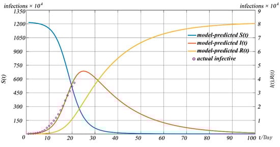
Figure 5.
Forecast of COVID-19 pandemic in China.
Table 3.
Model prediction results of .
In order to judge the pros and cons of fitting of the model, we choose the coefficient of determination as the criterion.
where , , and represents the actual value, the average and the predicted value of respectively. Based on the data from 20 January to 10 February, we obtained . It means that the fit explains 98.56% of the total variation in the actual data about the average in our model, which proves that the prediction results of our model are close to the real values of the pandemic situation, and the prediction has strong reference significance.
In addition, we drew the curves of removed individuals in China’s mainland based on official statistics, as shown in Figure 6.
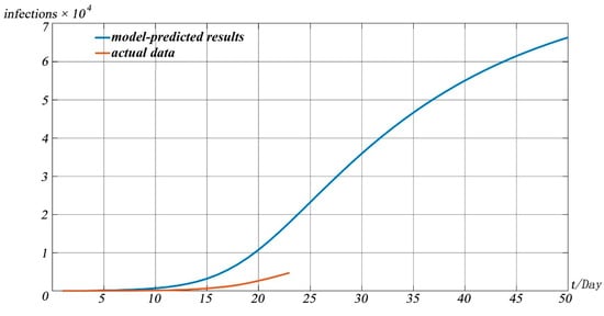
Figure 6.
The model-predicted cumulative number of removed individuals in China’s mainland.
It can be seen from Figure 6 that there is a certain time difference between the model and the real data in predicting the number of patients that were cured or died due to disease. That is, the real data arrive at a certain value later than the model predicts. However, the overall trend predicted by the models fits well with the real data. After analysis, we believe that this is mainly caused by the following reasons. First, the disease itself is a newly discovered disease, requiring a long treatment cycle, and many patients have a long recovery cycle, so the growth of the cured number in real statistics is relatively slow. At the same time, in the treatment process of the pandemic, the hospital has taken relatively cautious measures. After the symptoms disappear, the patients can be discharged only after two nucleic acid tests every two days, all negative, which also causes the number of cured patients to grow slowly.
Figure 7 shows the pandemic situation in Wuhan predicted by the model 50 days after 20 January 2020, and compares it with the real situation. In order to verify the difference between the model simulation results and the real situation, we simulated the number of confirmed cases in the whole process of the pandemic and compared them with the real situation of the pandemic. It can be seen from Figure 7 that the model is close to the real situation of the pandemic to a large extent, indicating the effectiveness of the model for pandemic prediction.
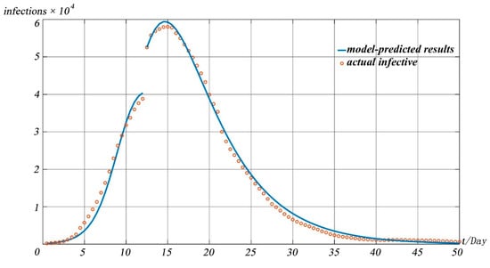
Figure 7.
Prediction curve and actual numbers of confirmed COVID-19 cases in China.
Since Wuhan is a transportation hub in central China, many provinces have a history of travel to Wuhan apparent in their imported cases. Therefore, we collected the nationwide number of confirmed cases from 20 January 2020 to 9 February 2020 [31], and drew the heat maps with an interval of five days as shown in Figure 8.
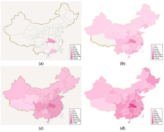
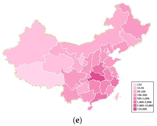
Figure 8.
Evolution of novel coronavirus in China with heat maps. (a–e) represent the pandemic situation on 20 January 2020, 25 January 2020, 30 January 2020, 4 February 2020, 9 February 2020, respectively.
As can be seen from Figure 8a–e, Hubei Province serves as the epicenter. The pandemic gradually spread to neighboring provinces over time. The number of confirmed cases is the highest in Hubei province and in neighboring provinces.
On this basis, we collected the ratio of the outflow population from other provinces to Hubei Province, respectively, in mainland China (excluding Hong Kong, Macao, and Taiwan) to the total outflow population of Hubei Province [32]. These data can reflect the population migration of Hubei during the development of the pandemic.
Based on the collated data, we drew a heat map of the passengers travelling from Hubei Province to various provinces, as shown in Figure 9. Comparing Figure 8 with Figure 9, we can find that the heat map of the national pandemic evolution is consistent with the population migration in mainland China from Hubei province. As a result, transportation can be considered the main channel for the spread of infectious diseases.
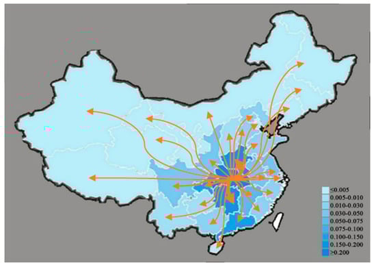
Figure 9.
Heat map of population migration in China’s mainland from Hubei Province.
3.2. Prediction Results Based on COVID-19 SIR Model of Nanjing
On the morning of 20 July 2021, the COVID-19 Prevention and Control Headquarters of Jiangning District, Nanjing received the special pandemic prevention team of the Lukou International Airport and reported that among the regular nucleic acid test samples of the staff of Lukou International Airport, the test results were positive, and the staff involved were mainly those involved in flight support at the airport, including those in ground service and cleaning positions. We used the model mentioned in Section 2 to simulate and predict the local pandemic in Nanjing.
The model takes the data of confirmed cases in Nanjing on 20 July 2021 as the initial value of the model, and the pandemic development trend chart shown in Figure 10 is obtained.
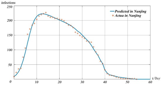
Figure 10.
The model-predicted infectious individuals in Nanjing.
It can be seen from Figure 10 that under the existing pandemic prevention and treatment measures in Nanjing, the pandemic peak will appear on 3 August 2021, and the peak number of infected people is about 223. We define Nanjing’s susceptible population as . Since the pandemic originated from a highly mobile and densely populated airport, increased significantly. It can be seen from Figure 10 that the prediction results of our model are close to the real data, indicating that the model in this paper can be equally applicable in small-scale pandemic situations.
In response to the prevention and control of the pandemic, relevant government departments have taken many measures. We conducted experiments based on our model to assess the impact of the measures taken by the government on the pandemic. The specific forecast results are shown in Figure 11.
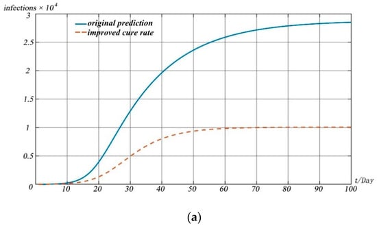
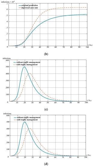
Figure 11.
Model simulations. (a) Change in recovered people with different cure rates; (b) change in deaths with different cure rates; (c) change in infected people with the impact of traffic management; (d) change in infected people with the impact of interventions.
When simulating the impact of different measures on the development of the pandemic, we simulated and predicted the possible impact of different pandemic prevention measures on the pandemic situation by adjusting the values of susceptible, infectious, and recovered cases in the model.
Figure 11 shows the impact of different prevention and control measures on the pandemic development for 100 days after 20 January 2020, as predicted by the model.
Figure 11a,b reflect the impact of drug research and development and treatment scheme improvement on the spread of the pandemic. With the introduction of measures such as drug research and development and improvement of treatment schemes, the cure rate of patients will be improved significantly and the death rate of diseases will be reduced greatly. We simulated the impact of drug research and development and the improvement of the treatment scheme on the pandemic situation by increasing the value of and reducing the value of . Simulation shows that the development of drugs and the improvement of treatment plan can lead to the peak of the pandemic in advance, and the number of infected people at the peak of the pandemic is lower than that without drugs and treatment measures.
Figure 11c reflects the impact of the implementation of traffic restriction measures in Wuhan based on pandemic prevention and control. The introduction of traffic restriction measures in many cities led by Wuhan City, Hubei Province can reduce vulnerable people to a certain extent. We assessed the impact of traffic restriction measures on the overall pandemic situation by reducing the value of . It can be found that the overall impact of the scheme on the pandemic situation is limited. That is, although the peak of the pandemic situation will decrease and move back to a certain extent, the degree of reduction of the peak is small, only about 100 people, and the time of the peak moving back is about 6 days.
In this pandemic situation, measures such as pandemic prevention publicity, popu-lation self-isolation, and reducing aggregation can significantly reduce susceptible populations. By significantly reducing the value, we evaluated the impact of various isola-tion measures on the development of the pandemic. As can be seen from Figure 11d, the above measures can significantly reduce the pandemic peak, and the date of the peak will be significantly delayed by about 25 days.
4. Discussion
Based on the published data on the pandemic situation and the cognition and research of medical experts on the pandemic situation, we draw the following conclusions with the help of an infectious disease dynamics model:
By using the SIR model designed in this paper and combining it with the pandemic data of China from 20 January 2020 to 31 January 2020, we simulated and predicted the pandemic development trend. This model is also applied to the prediction of the pandemic situation in Beijing. In different time ranges and geographical ranges, the method proposed in this paper can accurately predict the pandemic development. The specific results are as follows.
First, the number of infected people nationwide is expected to peak around 14 February 2020. The peak number of the pandemic was 45,737. Through the prediction and simulation of the whole process of pandemic development, it is concluded that the pandemic will gradually disappear after 100 days, and the number of infected people in the whole pandemic is about 80,284.
Second, for a large city such as Nanjing, pandemic prevention and control is accompanied by many uncertainties. The model predicted that the peak of the pandemic in Nanjing would appear in 3 August 2021, and the peak of the number of infected people would be about 223. The prediction results of the pandemic situation by the model are basically consistent with the actual development of the pandemic situation, and the pandemic trend curve is basically consistent with the actual number of confirmed cases.
This model simulates the change in the number of confirmed cases and the development trend of the pandemic situation, which is close to the national pandemic situation in early 2021 and the real development of the pandemic situation in Nanjing.
Using the simulation results of the pandemic development trend of the model in this paper, and combined with the prevention and control of a small-scale sporadic pandemic in the past two years, we draw the following conclusions:
The control of infectious diseases in the embryonic stage is considered the best time for pandemic prevention and control because it can cut off the transmission chain of the pandemic in a short time and effectively isolate the susceptible population from the confirmed population.
First, although Hubei may have missed the best time to curb the disease, the effective lockdown for several cities does have a largely positive effect at the later stage on prevention and control of the pandemic. These interventions can isolate infected people and limit their travel, so as to reduce the spread of the virus, which is significant when more and more people are infected in other areas.
Second, since the relevant pandemic prevention steps were taken, the effective spread rate of the pandemic has been better controlled across the country, and the cure rate of infected people has been greatly improved, while the mortality rate of infected people has been significantly reduced.
Third, isolation and observation of suspected populations is an important means of pandemic prevention and control, which can isolate susceptible populations from suspected populations as soon as possible. In addition, with the appeal from media and other channels, the general population go out less, try to avoid getting together and gathering for meals, and wear masks in and out of public places, which to a large extent, can limit the number of infected people and reduce the second-generation cases across the country, and perhaps the third generation, imported from Wuhan. These protections can prevent a large-scale outbreak even if transports suspension missed the best time to control the disease.
Although the pandemic in some areas appears to be at an inflection point, and the nationwide situation of pandemic prevention and control improves gradually, awareness and management still cannot be relaxed. With the large-scale population movement and the resumption of work in some enterprises and institutions after the end of the Spring Festival holiday in 2020, new challenges to the prevention and control of the pandemic may show up, and the second peak of the pandemic should be avoided.
Regardless of the types of disease, drug development, and therapy implementation are of help to treat and control the disease. Therefore, regarding this pandemic, front-line medical workers and researchers have made great contributions to the development and screening of drugs and treatment plans for pandemic prevention and control.
Our model implicates the importance of quarantine in pandemic prevention and control, but how to make more effective quarantine policies still needs further discussion. From the perspective of pandemic-spreading dynamics, only probable individuals need to be kept in quarantine. Therefore, if the detection equipment is sensitive and convenient enough, and people have a strong awareness of self-detection and isolation, theoretically speaking, the work and life of our society can nearly return to normal without pandemic freak-out. With respect to the protection of people’s livelihood, how to further improve the public health and strengthen the construction of infrastructure, and how to effectively regulate public transports and key public places are worthy to be noted by the relevant government departments so that they can prepare in advance and formulate specific feasible contingency plans in case of emergency.
The pandemic is different from individuals’ illness, for it brings great harm not only to people’s physical and mental health, but also to the politics, economics, culture, and education with respect to quality of life. For instance, due to the rapid spread of the disease, schools have postponed the new spring semester across the country. Additionally, some government departments get suspended, and the catering, tourism, entertainment industries, and transport companies may all suffer great losses. Meanwhile, small and medium-sized enterprises will have an enormous burden of survival crises. The magnitude of these impacts is difficult to accurately measure by numbers at this stage, and the elimination of these impacts cannot be completed overnight. A more complex calculation model is needed to evaluate the balance between pandemic prevention and control measures and various social elements.
As a consequence, from the perspective of social governance, how to strike a balance between effective pandemic control and the interests of the whole society is a more critical task.
5. Conclusions
Through the above research, it can be found that the relevant measures taken by the Chinese government in response to COVID-19 can play a key role in the rapid control and effective treatment of the pandemic. These measures have a certain reference value and significance for the upcoming Beijing Winter Olympics Organizing Committee in the organization of events, the isolation measures of foreign athletes, and the admission organization policies for spectators, which will provide a reference for the safety of large-scale events in worldwide.
Author Contributions
Conceptualization, Q.J. and H.M.; methodology, Q.L.; software, Y.L. and H.M.; validation, Q.G., Y.L. and Q.J.; formal analysis, X.Z. and Q.J.; investigation, Q.G. and Y.L.; resources, X.Z.; data curation, H.M. and Q.L.; writing—original draft preparation, Q.J.; writing—review and editing, Q.J., Y.L. and X.Z.; visualization, Q.J. and H.M.; supervision, X.Z.; project administration, X.Z. All authors have read and agreed to the published version of the manuscript.
Funding
This work was supported by the National Natural Science Foundation of China (grant numbers: 11801019).
Institutional Review Board Statement
Not applicable.
Informed Consent Statement
Not applicable.
Data Availability Statement
Data available in a publicly accessible repository.
Acknowledgments
The authors would like to thank the referees and editors for their very helpful and constructive comments, which have significantly improved the quality of this paper.
Conflicts of Interest
The authors declare there is no conflict of interest regarding the publication of this paper.
References
- Hu, Q.; Lu, R.; Peng, K.; Duan, X.; Wang, Y.; Zhao, Y.; Wang, W.; Lou, Y.; Tan, W. Prevalence and Genetic Diversity Analysis of Human Coronavirus OC43 among Adult Patients with Acute Respiratory Infections in Beijing, 2012. PLoS ONE 2014, 9, e100781. [Google Scholar] [CrossRef] [Green Version]
- Walls, A.C.; Xiong, X.; Park, Y.J.; Tortorici, M.A.; Snijder, J.; Quispe, J.; Cameroni, E.; Gopal, R.; Dai, M.; Lanzavecchia, A.; et al. Unexpected Receptor Functional Mimicry Elucidates Activation of Coronavirus Fusion. Cell 2019, 183, 1732. [Google Scholar] [CrossRef] [PubMed]
- Schäfer, A.; Baric, R.S. Epigenetic Landscape during Coronavirus Infection. Pathogens 2017, 6, 8. [Google Scholar] [CrossRef] [PubMed] [Green Version]
- Kelly-Cirino, C.; Mazzola, L.T.; Chua, A.; Oxenford, C.J.; Van Kerkhove, M.D. An Updated Roadmap for MERS-CoV Research and Product Development: Focus on Diagnostics. Br. Med. J. Glob. Health 2019, 4, e001105. [Google Scholar] [CrossRef] [PubMed] [Green Version]
- Website of the Xinhua News Agency. Available online: http://www.xinhuanet.com/2019-12/31/c_1125409031.htm (accessed on 1 June 2021).
- Tu, W.; Tang, H.; Chen, F.; Wei, Y.; Xu, T.; Liao, K.; Xiang, N.; Shi, G.; Li, Q.; Feng, Z. Epidemic Update and Risk Assessment of 2019 Novel Coronavirus—China. China CDC Wkly. 2020, 6, 83–86. [Google Scholar] [CrossRef]
- Balcha, A.A. Curve Fitting and Least Square Analysis to Extrapolate for the Case of COVID-19 Status in Ethiopia. Adv. Infect. Dis. 2020, 10, 143–159. [Google Scholar] [CrossRef]
- Website of the World Health Organization. Available online: https://www.who.int/emergencies/diseases/novel-coronavirus-2019 (accessed on 1 June 2021).
- Bernoulli, D. Essai D’une Nouvelle Analyse de la Mortalité Causée par la Petite Vérole et des Avantages de L’inoculation Pour la Prévenir, in Mémoires de Mathématiques et de Physique; Academie Royale des Sciences: Paris, France, 1760; pp. 1–45. [Google Scholar]
- Shulgin, B.; Stone, L.; Agur, Z. Pulse vaccination strategy in the SIR epidemic model. Bull. Math. Biol. 1998, 60, 1123–1148. [Google Scholar] [CrossRef]
- Lekone, P.E.; Finkenstädt, B.F. Statistical Inference in a Stochastic Epidemic SEIR Model with Control Intervention: Ebola as a Case Study. Biometrics 2006, 62, 1170–1177. [Google Scholar] [CrossRef] [PubMed] [Green Version]
- Talawar, A.S.; Aundhakar, U. Parameter Estimation of SIR Epidemic Model using MCMC Methods. Glob. J. Pure Appl. Math. 2016, 12, 1299–1306. [Google Scholar]
- Florea, A.; Lăzureanu, C. A Mathematical Model of Infectious Disease Transmission. Available online: https://www.proquest.com/openview/42bebdcd76c4808d2d47653b48baab26/1?pq-origsite=gscholar&cbl=2040552 (accessed on 1 June 2021).
- Zhang, Y.; Liu, X.; Cai, C.; Jia, Z. Model of Transmission of Infectious Diseases Based on Traffic Network. Comput. Digit. Eng. 2017, 45, 2359–2363. [Google Scholar]
- The Content Column of “Epidemic Prevention and Control Trends” on the Official Website of the National Health Commission. Available online: http://www.nhc.gov.cn/xcs/yqfkdt/gzbd_index.shtml (accessed on 1 June 2021).
- Kermack, W.O.; McKendrick, A.G. A Contribution to the Mathematical Theory of Epidemics. Proc. R. Soc. Lond. Ser. A Contain. Pap. Math. Character 1927, 115, 700–721. [Google Scholar]
- Law, K.B.; Peariasamy, K.M.; Gill, B.S.; Singh, S.; Sundram, B.M.; Rajendran, K.; Dass, S.C.; Lee, Y.L.; Goh, P.P.; Ibrahim, H.; et al. Tracking the Early Depleting Transmission Dynamics of COVID-19 with a Time-varying SIR Model. Sci. Rep. 2020, 10, 21721. [Google Scholar] [CrossRef]
- Rafieenasab, S.; Zahiri, A.P.; Roohi, E. Prediction of Peak and Termination of Novel Coronavirus COVID-19 Epidemic in Iran. Int. J. Mod. Phys. C 2020, 31, 2050152. [Google Scholar] [CrossRef]
- Moraes, A.L.S.; Monteiro, L.H. On Considering the Influence of Recovered Individuals in Disease Propagations-ScienceDirect. Commun. Nonlinear Sci. Numer. Simul. 2016, 34, 224–230. [Google Scholar] [CrossRef]
- Chinazzi, M.; Davis, J.T.; Ajelli, M.; Gioannini, C.; Litvinova, M.; Merler, S.; Piontti, A.P.Y.; Mu, K.; Rossi, L.; Sun, K.; et al. The effect of travel restrictions on the spread of the 2019 novel coronavirus (COVID-19) outbreak. Science 2020, 368, 395–400. [Google Scholar] [CrossRef] [Green Version]
- Cornbleet, P.J.; Gochman, N. Incorrect Least-squares Regression Coefficients in Method-comparison Analysis. Clin. Chem. 1979, 25, 432–438. [Google Scholar] [CrossRef]
- Zhou, T.; Liu, Q.; Yang, Z.; Liao, J.; Yang, K.; Bai, W.; Lu, X.; Zhang, W. Preliminary Prediction of the Basic Reproduction Number of the Wuhan Novel Coronavirus 2019-nCoV. J. Evid.-Based Med. 2020, 13, 3–7. [Google Scholar] [CrossRef]
- Anderson, R.M.; May, R.M. Infectious Diseases of Humans; Oxford University Press: New York, NY, USA, 1991. [Google Scholar]
- Hattaf, K.; Lashari, A.; Louartassi, Y.; Yousfi, N. A Delayed SIR Epidemic Model with General Incidence Rate. Electr. J. Qual. Theory Differ. Equ. 2013, 3, 1–9. [Google Scholar] [CrossRef]
- Bai, Z.G. Basic Reproduction Number of Periodic Epidemic Models. Chin. J. Eng. Math. 2013, 30, 175–183. [Google Scholar]
- Van den Driessche, P.; Watmough, J. Reproduction Numbers and Sub-threshold Endemic Equilibria for Compartmental Models of Disease. Math. Biosci. 2002, 180, 29–48. [Google Scholar] [CrossRef]
- Nabi, G.; Khan, S. Novel Coronavirus Transmission to Water Bodies; Risk of COVID-19 Pneumonia to Aquatic Mammals. Environ. Res. 2020, 188, 109732. [Google Scholar] [CrossRef]
- Website of the Yangtze River Network. Available online: http://news.cjn.cn/sywh/202002/t3574262.htm (accessed on 1 June 2021).
- Oran, D.P.; Topol, E.J. Prevalence of Asymptomatic SARS-CoV-2 Infection. Ann. Intern. Med. 2021, 174, 286–287. [Google Scholar] [CrossRef] [PubMed]
- Website of the National Health Committee of the People’s Republic of China. Available online: http://www.nhc.gov.cn/xcs/yqtb/202001/a5f1aec0660f4cd3a70518b6258fd15f.shtml (accessed on 1 June 2021).
- Website of the Central People’s Government of the People’s Republic of China. Available online: http://www.gov.cn/fuwu/zt/yqfwzq/zxqk.htm#0 (accessed on 1 June 2021).
- Website of the Baidu Map Insight. Available online: https://qianxi.baidu.com/ (accessed on 1 June 2021).
Publisher’s Note: MDPI stays neutral with regard to jurisdictional claims in published maps and institutional affiliations. |
© 2021 by the authors. Licensee MDPI, Basel, Switzerland. This article is an open access article distributed under the terms and conditions of the Creative Commons Attribution (CC BY) license (https://creativecommons.org/licenses/by/4.0/).