
Comparison of Molecular Geometry Optimization Methods Based on Molecular Descriptors


Abstract
1. Introduction
- 6-31G → cc-pVDZ
- 6-311G → aug-cc-pVDZ
- 6-31+G(d) → cc-pVTZ
- 6-311+G(d) → aug-cc-pVTZ
- 6-31++G(d,p) → cc-pVQZ
- 6-311++G(d,p) → aug-cc-pVQZ
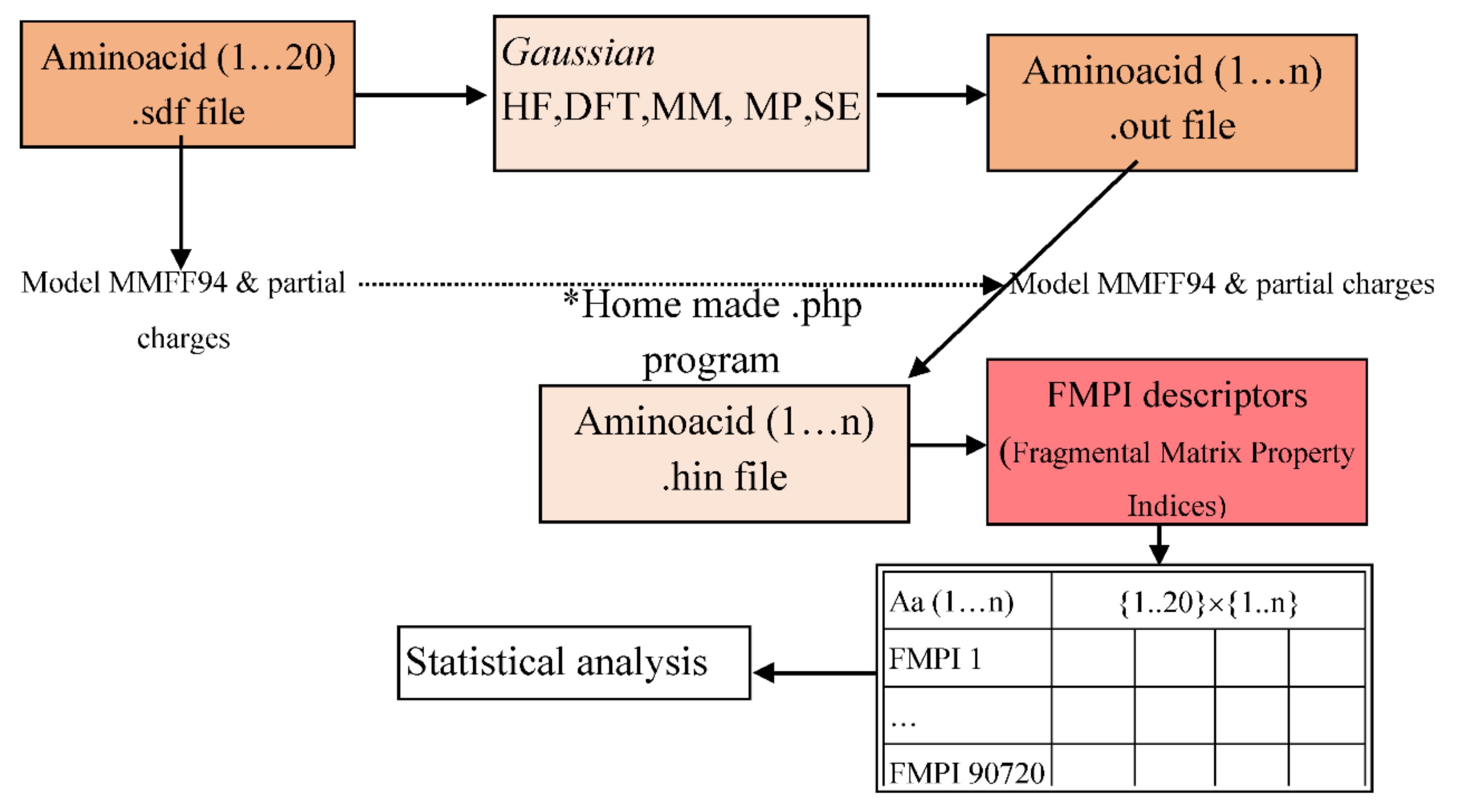
2. Materials and Methods
- Enter the PubChem .sdf files to the Gaussian program.
- Save the file in .gjf file format (the input file format for the program).
- Analyse the amino acids using the following t command: Calculate → Gaussian Calculation Setup → Job type (Optimization).
- From the Calculation Setup menu select the Gaussian Geometry Optimization Methods one after another and run the calculations.
- Save for every calculation the .out file (the output file format for the program).
3. Results and Discussion
4. Conclusions
Author Contributions
Funding
Institutional Review Board Statement
Informed Consent Statement
Conflicts of Interest
References
- Slater, J.C. Atomic Shielding Constants. Phys. Rev. 1930, 36, 57. [Google Scholar] [CrossRef]
- Boys, S.F. Electronic Wave Functions. I. A General Method of Calculation for the Stationary States of any Molecular System. Proc. R. Soc. 1950, 200, 542–554. [Google Scholar]
- Joiţa, D.-M.; Tomescu, M.A.; Bàlint, D.; Jäntschi, L. An Application of the Eigenproblem for Biochemical Similarity. Symmetry 2021, 13, 1849. [Google Scholar] [CrossRef]
- Jäntschi, L. The Eigenproblem Translated for Alignment of Molecules. Symmetry 2019, 11, 1027. [Google Scholar] [CrossRef]
- Schrödinger, E. An Undulatory Theory of the Mechanics of Atoms and Molecules. Phys. Rev. 1926, 8, 1049–1070. [Google Scholar] [CrossRef]
- Abegg, P.W.; Ha, T.-K. Ab initio calculation of spin-orbit-coupling constant from Gaussian lobe SCF molecular wavefunctions. Mol. Phys. 1974, 27, 763–767. [Google Scholar] [CrossRef]
- Binkley, J.S.; Pople, J.A.; Hehre, W.J. Self-consistent Molecular Orbital Methods. Small Split-valence Basis Sets for First-row Elements. J. Am. Chem. Soc. 1980, 102, 939–947. [Google Scholar] [CrossRef]
- Gordon, M.S.; Stephen, B.J.; Pople, J.A.; Pietro, W.J.; Hehre, W.J. Self-consistent Molecular-orbital Methods. Small Split-valence Basis Sets for Second-row Elements. J. Am. Chem. Soc. 1982, 104, 2797–2803. [Google Scholar] [CrossRef]
- Pietro, W.J.; Francl, M.M.; Hehre, W.J.; DeFrees, D.J.; Pople, J.A.; Binkley, J.S. Self-consistent Molecular Orbital Methods. Supplemented Small Split-valence Basis Sets for Second-row Elements. J. Am. Chem. Soc. 1982, 104, 5039–5048. [Google Scholar] [CrossRef]
- Pople, J.A. Quantum Chemical Models. Angew. Chem. 1999, 38, 13–14. [Google Scholar] [CrossRef]
- Ditchfield, R.; Hehre, W.J.; Pople, J.A. Self-Consistent Molecular-Orbital Methods. IX. An Extended Gaussian-Type Basis for Molecular-Orbital Studies of Organic Molecules. J. Chem. Phys. 1971, 54, 724–728. [Google Scholar] [CrossRef]
- Banerjee, T.; Ramalingam, A. Molecular Modeling and Optimization. In Desulphurization and Denitrification of Diesel Oil Using Ionic Liquids: Experiments and Quantum Chemical Predictions; Elsevier: Amsterdam, The Netherlands, 2015; pp. 11–38. [Google Scholar]
- Hohenberg, P.; Kohn, W. Inhomogeneous Electron Gas. Phys. Rev. 1964, 136, B864. [Google Scholar] [CrossRef]
- Diudea, M.V.; Gutman, I.; Jäntschi, L. Molecular Topology; Nova Science Publishers: New York, NY, USA, 2002. [Google Scholar]
- Petersson, G.A.; Malick, D.K.; Wilson, W.G.; Ochterski, J.W.; Montgomery, J.A., Jr.; Frisch, M.J. Calibration and comparison of the Gaussian-2, complete basis set, and density functional methods for computational thermochemistry. J. Chem. Phys. 1998, 109, 10570–10579. [Google Scholar] [CrossRef]
- Scuseria, G.E. Comparison of coupled-cluster results with a hybrid of Hartree-Fock and density functional theory. J. Chem. Phys. 1992, 97, 7528–7530. [Google Scholar] [CrossRef]
- Zheng, G.; Irle, S.; Morokuma, K. Performance of the DFTB method in comparison to DFT and semiempirical methods for geometries and energies of C20-C86 fullerene isomers. Chem. Phys. Lett. 2005, 412, 210–216. [Google Scholar] [CrossRef]
- Hill, J.G. Gaussian basis sets for molecular applications. Int. J. Quantum Chem. 2012, 113, 21–34. [Google Scholar] [CrossRef]
- Spies, M. Transducer field modeling in anisotropic media by superposition of Gaussian base functions. J. Nondestruct. J. Acoust. Soc. Am. 1999, 105, 633. [Google Scholar] [CrossRef]
- Kayano, M.; Dozono, K.; Konishi, S. Functional Cluster Analysis via Orthonormalized Gaussian Basis Expansions and Its Application. J. Classif. 2010, 27, 211–230. [Google Scholar] [CrossRef]
- Available online: https://pubchem.ncbi.nlm.nih.gov/ (accessed on 5 September 2021).
- Jäntschi, L.; Bolboaca, S. Molecular modeling in compounds series with descriptors families. An. Univ. Oradea Fasc. Chim. 2016, 23, 5–14. [Google Scholar]
- Bolboacă, S.D.; Jäntschi, L. Nano-quantitative structure-property relationship modeling on C42 fullerene isomers. J. Chem. 2016, 1, 1. [Google Scholar] [CrossRef]
- Jäntschi, L. Predicţia Proprietăţilor Fizico-Chimice Şi Biologice Cu Ajutorul Descriptorilor Matematici. Ph.D. Thesis, Universitatea “Babeş-Bolyai” din Cluj-Napoca, Cluj-Napoca, Romania, 2000. [Google Scholar]
- Scott, A.P.; Radom, L. Harmonic Vibrational Frequencies: An Evaluation of Hartree-Fock, Møller-Plesset, Quadratic Configuration Interaction, Density Functional Theory, and Semiempirical Scale Factors. J. Phys. Chem. 1996, 100, 16502–16513. [Google Scholar] [CrossRef]
- Batra, P.; Bernd, G.; Gescheidt, M.S.G.; Houk, K.N. Calculations of Isotropic Hyperfine Coupling Constants of Organic Radicals. An Evaluation of Semiempirical, Hartree-Fock, and Density Functional Methods. J. Phys. Chem. 1996, 100, 18371–18379. [Google Scholar] [CrossRef]
- Russ, N.J.; Crawford, T.D.; Tschumper, G.S. Real versus artifactual symmetry-breaking effects in Hartree–Fock, density-functional, and coupled-cluster methods. J. Chem. Phys. 2004, 120, 7298. [Google Scholar] [CrossRef] [PubMed][Green Version]
- Davidson, E.R.; Feller, D. Basis Set Selection for Molecular Calculations. Chem. Rev. 1988, 86, 661–696. [Google Scholar] [CrossRef]
- Cramer, C.J. Essentials of Computational Chemistry: Theories and Models; John Wiley and Sons, Ltd.: Hoboken, NJ, USA, 2002. [Google Scholar]
- Pople, J.A.; Beveridge, D.L.; Dobosh, P.A. Approximate Self-Consistent Molecular-Orbital Theory. Intermediate Neglect of Differential Overlap. J. Chem. Phys. 1967, 47, 2026. [Google Scholar] [CrossRef]
- Dunning, T.H. Gaussian basis sets for use in correlated molecular calculations. The atoms boron through neon and hydrogen. J. Chem. Phys. 1989, 90, 1007. [Google Scholar] [CrossRef]
- Stewart, J.J.P. Optimization of parameters for semiempirical methods. Applications. J. Comput. Chem. 1989, 10, 221. [Google Scholar] [CrossRef]
- Jensen, F. Atomic orbital bases sets. WIREs Comput. Mol. Sci. 2012, 3, 273–295. [Google Scholar] [CrossRef]
- Jäntschi, L. Computer assisted geometry optimization for in silico modeling. Appl. Med. Inform. 2011, 29, 11–18. [Google Scholar]


| Amino Acids (AA) | |||
|---|---|---|---|
| Arginine | Lysine | Methionine | Leucine |
| Asparagine | Serine | Alanine | Phenylalanine |
| Aspartate | Threonine | Valine | Proline |
| Glutamate | Cysteine | Glycine | Tryptophan |
| Glutamine | Histidine | Isoleucine | Tyrosine |
| Gaussian Optimization Methods | |
|---|---|
| Semi-Empirical Methods (Default Spin) | 1. Parameterized Model 6 PM6 (opt-pm6) 2. Austin Model 1 AM1 (opt-am1) 3. Parameterized Model 3 PM3 (opt-pm3) 4. Parameterized Model 3 (Molecular Mechanics correction) PM3MM (opt-pm3mm) 5. Pairwise Distance Directed Gaussian function PDDG (opt-pddg) 6. Complete Neglect of Differential Overlap CNDO (opt-cndo) 7. Intermediate Neglect of Differential Overlap INDO (opt-indo) |
| Density Functional Theory (Default Spin) | Becke(three-parameter)–Lee–Yang–Parr (functional) B3LYP 8. opt-b3lyp-sto-3g; 9. opt-b3lyp-3-21g; 10. opt-b3lyp-6-31g; 11. opt-b3lyp-6-311g; 12. opt-b3lyp-cc-pvdz;) Local Spin Density Approximation LSDA 13. opt-lsda-3-21g; 14. opt-lsda-sto-3g; 15. opt-lsda-cc-pvdz; 16. opt-lsda-6-311g; 17. opt-lsda-6-31g;) 18. Perdew–Burke-Ernzerhof (functional) PBEPBE opt-pbepbe-sto-3g BVP86 19. opt-bvp86-sto-3g; 20. opt-bvp86-3-21g; 21. Opt-bvp86-6-31g; 22. opt-bvp86-6-311g;) B3PW91 23. opt-b3pw91-sto-3g; 24. opt-b3pw91-6-31g; 25. opt-b3pw91-6-311g;) |
| Møller–Plesset Perturbation Theory | MP2 26. opt-mp2-sto-3g; 27. opt-mp2-3-21g; 28. opt-mp2-6-31g; 29. opt-mp2-6-311g; 30. opt-mp2-cc-pvdz;) |
| Coupled-Cluster Theory | 31. Coupled Cluster single-double CCSD (opt-ccsd-sto-3g) |
| Molecular Mechanics (Default Spin) | 32. Universal Force Field UFF (opt-uff) 33. Dreiding (opt-dreiding) |
| Hartree–Fock (Default Spin) | 34.STO-3G(opt-hf-sto-3g) 35.3-21G(opt-hf-3-21g) 36.3-21G*(opt-hf-3-21g*) 37.6-31G(opt-hf-6-31g) 38.6-311G(opt-hf-6-311g) 39.CC-pvdz(opt-hf-cc-pvdz) |
Publisher’s Note: MDPI stays neutral with regard to jurisdictional claims in published maps and institutional affiliations. |
© 2021 by the authors. Licensee MDPI, Basel, Switzerland. This article is an open access article distributed under the terms and conditions of the Creative Commons Attribution (CC BY) license (https://creativecommons.org/licenses/by/4.0/).
Share and Cite
Bálint, D.; Jäntschi, L. Comparison of Molecular Geometry Optimization Methods Based on Molecular Descriptors. Mathematics 2021, 9, 2855. https://doi.org/10.3390/math9222855
Bálint D, Jäntschi L. Comparison of Molecular Geometry Optimization Methods Based on Molecular Descriptors. Mathematics. 2021; 9(22):2855. https://doi.org/10.3390/math9222855
Chicago/Turabian StyleBálint, Donatella, and Lorentz Jäntschi. 2021. "Comparison of Molecular Geometry Optimization Methods Based on Molecular Descriptors" Mathematics 9, no. 22: 2855. https://doi.org/10.3390/math9222855
APA StyleBálint, D., & Jäntschi, L. (2021). Comparison of Molecular Geometry Optimization Methods Based on Molecular Descriptors. Mathematics, 9(22), 2855. https://doi.org/10.3390/math9222855