Study of a Modified Kumaraswamy Distribution

Abstract

In this article, a structural modification of the Kumaraswamy distribution yields a new two-parameter distribution defined on $(0,1)$, called the modified Kumaraswamy distribution. It has the advantages of being (i) original in its definition, mixing logarithmic, power and ratio functions, (ii) flexible from the modeling viewpoint, with rare functional capabilities for a bounded distribution—in particular, N-shapes are observed for both the probability density and hazard rate functions—and (iii) a solid alternative to its parental Kumaraswamy distribution in the first-order stochastic sense. Some statistical features, such as the moments and quantile function, are represented in closed form. The Lambert function and incomplete beta function are involved in this regard. The distributions of order statistics are also explored. Then, emphasis is put on the practice of the modified Kumaraswamy model in the context of data fitting. The well-known maximum likelihood approach is used to estimate the parameters, and a simulation study is conducted to examine the performance of this approach. In order to demonstrate the applicability of the suggested model, two real data sets are considered. As a notable result, for the considered data sets, statistical benchmarks indicate that the new modeling strategy outperforms the Kumaraswamy model. The transmuted Kumaraswamy, beta, unit Rayleigh, Topp–Leone and power models are also outperformed.

1. Introduction

The perfect modeling of random processes that one regularly observes in applied sciences remains in the order of utopia. Scientists and practitioners have already discussed a wide range of models for solving these challenges. When the processes take values in the interval $(0,1)$, a primary statistical analysis can be performed with the standard beta and Kumaraswamy (Kw) models. Before going further, a retrospective on these models is necessary. First, they are derived from the beta and Kw distributions, respectively. The beta distribution is a continuous distribution with support on the interval $(0,1)$ and parameterized by two positive shape parameters, $\alpha$ and $\beta$. It is mathematically defined by the following cumulative distribution function (cdf):

$$F_{beta}(x;\alpha ,\beta )=\frac{1}{B(\alpha ,\beta )}{\int }_0^x{t}^{\alpha -1}{(1-t)}^{\beta -1}dt,x\in (0,1),$$

where $B(\alpha ,\beta )={\int }_0^1{t}^{\alpha -1}{(1-t)}^{\beta -1}dt$, $F_{beta}(x;\alpha ,\beta )=0$ for $x\le 0$, and $F_{beta}(x;\alpha ,\beta )=1$ for $x\ge 1$. Naturally, the values of $\alpha$ and $\beta$ influence the shape of the distribution. The corresponding probability density function (pdf) can be U-shaped, bell-shaped, monotonic (increasing or decreasing), or even straight lines. On the other hand, the corresponding hazard rate function (hrf) can be increasing with convex shapes, or U-shaped (see [1,2]). In a wide number of areas, the beta distribution is used to model the behavior of characteristics representing percentages and proportions. See, for example, the developments in [3].

In [4], the Kw distribution was introduced to complement the beta distribution. Thus, it is also a continuous distribution with support in $(0,1)$ and parameterized by two positive shape parameters, $\alpha$ and $\beta$. The Kw distribution is conceptually based on uniform order statistics, and it has extremely simple functions that do not rely on special functions. The cdf of the Kw distribution is given as follows:

$$F_{Kw}(x;\alpha ,\beta )=1-{(1-x^{\beta })}^{\alpha },x\in (0,1),$$

where $F_{Kw}(x;\alpha ,\beta )=0$ for $x\le 0$, and $F_{Kw}(x;\alpha ,\beta )=1$ for $x\ge 1$. The form of the functions related to this distribution is naturally influenced by the values of $\alpha$ and $\beta$. Its application domain is identical to that of the beta distribution. As a brief comparison, the Kw distribution is similar to the beta distribution, but it is much easier to work with thanks to the tractability of its functions. We refer the reader to [5] and the references therein for more information on this claim. As a fact, the beta and Kw models rarely achieve the goal of optimal performance in all cases. For these reasons, new models on the unit intervals have been proposed, derived from new distributions with support equal to $(0,1)$. These distributions are more or less sophisticated in the analytical sense. Contemporary works on this topic can be found in [6,7,8,9,10,11,12,13,14,15,16,17,18,19].

In this article, we propose a new two-parameter unit distribution, called the modified Kumaraswamy (MKw) distribution. The considered cdf is such that, for $x\in (0,1)$, the following holds:

$$F_{MKw}(x;\alpha ,\beta )=1-T\left[{(1-x^{\beta })}^{\alpha }\right],$$

where $T\left(x\right)$ denotes a certain analytical transformation that will be presented later. At this introductory step, some features of $T\left(x\right)$ are listed below.

Feature I.

First of all, the transformation $T\left(x\right)$ has an original form involving polynomial and logarithmic functions without additional parameters. Thanks to it, some functional capabilities of the Kw distribution are extended or modified, and can be more adapted in some practical situations. In particular, the pdf of the MKw distribution can be monotonic in a nearly angular way, “strongly” left- or right-skewed and of a leptokurtic nature, or N-shaped. To our knowledge, these properties are not observed for the pdf of the Kw distribution. On the other hand, the corresponding hrf presents a wide panel of non-monotonic shapes, including N-shapes, that the hrf of the Kw distribution does not possess. All these curvature differences give credit for a more in-depth investigation of the MKw distribution from the modeling viewpoint.

Feature II.

The transformation $T\left(x\right)$ increases with respect to x. Thus, the intrinsic first-order stochastic dominance (FOS) properties of the Kw distribution can be transposed to the MKw distribution: for any $0<{\alpha }_1\le {\alpha }_2$ and $0<{\beta }_1\le {\beta }_2$, we have $F_{MKw}(x;{\alpha }_1,{\beta }_2)\le F_{MKw}(x;{\alpha }_2,{\beta }_1)$ for any $x\in \mathbb{R}$.

Feature III.

The transformation $T\left(x\right)$ satisfies the following inequality: $T\left(x\right)\ge x$ for any $x\in (0,1)$. Thanks to it, the Kw and MKw distributions are involved in a simple FOS dominance result: $F_{MKw}(x;\alpha ,\beta )\le F_{Kw}(x;\alpha ,\beta )$ for any $x\in \mathbb{R}$. This means that the MKw distribution generates a two-parameter statistical model, which does not intersect with the Kw model in the cdf sense.

In fact, several mathematical interpretations of the MKw distribution are possible. For instance, the MKw distribution may be viewed as a special parametric weighted version of the Kw distribution. Additionally, it is deeply connected with the ratio power-logarithmic (RPL) distribution created by [20]. Thanks to this connection, some properties of the RPL distribution may be used to determine those of the MKw distribution, among other things. These diverse interpretations are detailed in the first part of the paper, along with some theoretical properties. These properties include detailed quantile and moment analyses, illustrated numerically and graphically for some selected values of $\alpha$ and $\beta$. The order statistics are also discussed. The second part is devoted to the modeling characteristics of the MKw distribution. The MKw model is considered, assuming that the parameters $\alpha$ and $\beta$ are unknown, and may be estimated via available data. We examine the estimation of these parameters by the maximum likelihood method. We show the efficiency of the obtained estimates by the use of simulated data. Then, two different data sets are analyzed, and comparisons are made between the fits of the NKw, Kw, and beta models and four other referenced models of the literature. We show that the proposed MKw model outperforms the concurrence through the use of standard statistical benchmarks. The findings are illustrated by numerous graphics.

The organization of the paper is composed of the following section. Section 2 introduces the MKw distribution with full details, along with a functional analysis of the pdf and hrf. Section 3 is devoted to quantile analysis and moment analysis. The statistical inference on the parameters is considered in Section 4. Section 5 is devoted to applications. We end the paper with a concluding part in Section 6.

2. The Modified Kw Distribution

This section focuses on the MKw distribution and its basic functional features.

2.1. Primary Definition

The following mathematical result is at the basis of the MKw distribution.

Proposition 1.

Let $\alpha >0$ and $\beta >0$, and $G(x;\alpha ,\beta )$ be the function defined on $\mathbb{R}$ by

$$G(x;\alpha ,\beta )=1-\frac{{(1-x^{\beta })}^{\alpha }-1}{\alpha ln(1-x^{\beta })},x\in (0,1),$$

$G(x;\alpha ,\beta )=0$ for $x\le 0$, and $G(x;\alpha ,\beta )=1$ for $x\ge 1$. Thus defined, $G(x;\alpha ,\beta )$ has the required properties of a continuous cdf.

Proof. 

First, it is clear that $G(x;\alpha ,\beta )$ is continuous on $\mathbb{R}\{0,1\}$. Let us examine its behavior at the particular points $x=0$ and $x=1$. At the neighborhood of $x=0$, by virtue of standard equivalence functions, we have the following:

$$G(x;\alpha ,\beta )=1-\frac{{(1-x^{\beta })}^{\alpha }-1}{\alpha ln(1-x^{\beta })}\sim 1-\frac{-\alpha x^{\beta }}{\alpha (-x^{\beta })}=0=G(0;\alpha ,\beta ),$$

and, at the neighborhood of $x=1$, we have

$$G(x;\alpha ,\beta )=1-\frac{{(1-x^{\beta })}^{\alpha }-1}{\alpha ln(1-x^{\beta })}\sim 1+\frac{1}{\alpha ln(1-x^{\beta })}\to 1=G(1;\alpha ,\beta ).$$

Therefore, $G(x;\alpha ,\beta )$ is continuous on $\{0,1\}$, and on $\mathbb{R}$. By construction, we have ${lim}_{x\to -\infty }G(x;\alpha ,\beta )=0$ and ${lim}_{x\to +\infty }G(x;\alpha ,\beta )=1$. Let us now prove that $G(x;\alpha ,\beta )$ is increasing. By applying standard rules of differentiation, for $x\in (0,1)$, we obtain the following:

$$\begin{array}{c}\hfill G^{\prime }(x;\alpha ,\beta )=\frac{\beta x^{\beta -1}\left[{(1-x^{\beta })}^{\alpha }(1-\alpha ln(1-x^{\beta }))-1\right]}{\alpha (x^{\beta }-1){[ln(1-x^{\beta })]}^2}.\end{array}$$

(1)

The famous logarithmic inequality $ln(1+y)\ge y/(1+y)$ for $y>-1$, with $y={(1-x^{\beta })}^{\alpha }-1>-1$ yields the following:

$$\begin{array}{c}\hfill \alpha ln(1-x^{\beta })=ln\left[1+{(1-x^{\beta })}^{\alpha }-1\right]\ge \frac{{(1-x^{\beta })}^{\alpha }-1}{1+{(1-x^{\beta })}^{\alpha }-1}=1-{(1-x^{\beta })}^{-\alpha }.\end{array}$$

(2)

This inequality can be rearranged as ${(1-x^{\beta })}^{\alpha }(1-\alpha ln(1-x^{\beta }))-1\le 0$. Therefore, the numerator in Equation (1) is negative. Since the denominator is also negative, we have $G^{\prime }(x;\alpha ,\beta )\ge 0$, implying that $G(x;\alpha ,\beta )$ is increasing. This concludes the proof of Proposition 1. □

To the best of our knowledge, the cdf presented in Proposition 1 is new in the literature. It defines a modified version of the Kw distribution, described as the MKw distribution, discussed in Section 1. Some mathematical interpretations of this distribution are important to understand why the term “modified” is employed here. This is developed in the next section.

2.2. Mathematical Interpretations

Thus, the cdf of the MKw distribution is defined by the following:

$$\begin{array}{c}\hfill F_{MKw}(x;\alpha ,\beta )=1-\frac{{(1-x^{\beta })}^{\alpha }-1}{\alpha ln(1-x^{\beta })},x\in (0,1),\end{array}$$

(3)

where $F_{MKw}(x;\alpha ,\beta )=0$ for $x\le 0$, and $F_{MKw}(x;\alpha ,\beta )=1$ for $x\ge 1$, with $\alpha >0$ and $\beta >0$. Some mathematical interpretations of this cdf are given below.

Interpretation 1.

As sketched in Section 1, for $x\in (0,1)$, we can write the following:

$$F_{MKw}(x;\alpha ,\beta )=1-T\left[{(1-x^{\beta })}^{\alpha }\right],$$

with $T\left(x\right)=(x-1)/ln\left(x\right)$. In this sense, the transformation $T\left(x\right)$ modifies the mathematical structure of the cdf of the Kw distribution for different modeling perspectives.

The following facts can be deduced from the well-known logarithmic inequality $ln(1+y)\ge y/(1+y)$ for $y>-1$ when applied to $y=x-1$:

• $T^{\prime }\left(x\right)=(xln\left(x\right)+1-x)/\left[x{(ln\left(x\right))}^2\right]\ge 0$. This implies that $T\left(x\right)$ is an increasing function with respect to x. Following this is the stochastic FOS property: for any $0<{\alpha }_1\le {\alpha }_2$ and $0<{\beta }_1\le {\beta }_2$, we have $F_{MKw}(x;{\alpha }_1,{\beta }_2)\le F_{MKw}(x;{\alpha }_2,{\beta }_1)$ for any $x\in \mathbb{R}$.
• $T\left(x\right)=(x-1)/ln\left(x\right)\ge x$ for any $x\in (0,1)$. This implies that $F_{MKw}(x;\alpha ,\beta )\le F_{Kw}(x;\alpha ,\beta )$ for any $x\in \mathbb{R}$. In other words, there is a direct FOS dominance of the MKw distribution over the Kw distribution.

At the neighborhood of $x=0$, we have $T\left(x\right)\sim -1/ln\left(x\right)\to 0$. This convergence is slow, compared to the polynomial convergence to 0. This asymptotic result plays an important role to understand the possible difference in the right skewness between the MKw and Kw distributions; without more investigation, from the statistical viewpoint, it is natural to think that the MKw model is more able to capture the slow right-decay of a phenomena that the Kw model. This will be confirmed later with a skewness analysis through quantile and moment methods, as well as practical data.

Interpretation 2.

As a twin viewpoint, for $x\in (0,1)$, we can write the following:

$$F_{MKw}(x;\alpha ,\beta )=1-w(x;\alpha ,\beta ){(1-x^{\beta })}^{\alpha },$$

with $w(x;\alpha ,\beta )=[1-{(1-x^{\beta })}^{-\alpha }]/[\alpha ln(1-x^{\beta })]$. Thus, the weight function $w(x;\alpha ,\beta )$ modulate the main polynomial term of the cdf of the Kw distribution. In this sense, the MKw distribution is a weighted version of the Kw distribution.

Interpretation 3.

There is a deep relationship between the MKw and RPL distributions. First, we recall that the RPL distribution is defined by the following logarithmic-power cdf:

$$\begin{array}{c}\hfill F_{RPL}(x;\alpha )=\frac{x^{\alpha }-1}{\alpha ln\left(x\right)},x\in (0,1),\end{array}$$

$F_{RPL}(x;\alpha )=0$ for $x\le 0$ and $F_{RPL}(x;\alpha )=1$ for $x\ge 1$. Then, for a random variable Y following the RPL distribution, the random variable $X={(1-Y)}^{1/\beta }$ follows the MKw distribution. Indeed, for $x\in (0,1)$, we have the following:

$$\begin{array}{cc}\hfill P(X\le x)& =P({(1-Y)}^{1/\beta }\le x)=P(1-Y\le x^{\beta })=P(Y\ge 1-x^{\beta })\hfill \\ \hfill & =1-F_{RPL}(1-x^{\beta };\alpha )=F_{MKw}(x;\alpha ,\beta ).\hfill \end{array}$$

By identification, the stated result is obtained. Thanks to the representation of X, some properties of the RPL distribution can be used to determine those of the MKw distribution.

Finally, because any random variable X defined on $(0,1)$ can be shifted to a bounded support of the form $(a,b)$ with $a<b$, using the transformation $(b-a)X+a$, the MKw distribution can easily be extended to any bounded domain.

2.3. Functional Analysis

This part is devoted to a functional analysis of the main functions of the MKw distribution. To begin, we recall that the cdf of the MKw distribution is given by Equation (3). As any cdf, it is an increasing function. Some asymptotic results are now presented. In the neighborhood of $x=0$, by virtue of standard equivalence functions at orders of 1 or 2, we have the following:

$$F_{MKw}(x;\alpha ,\beta )=1-\frac{{(1-x^{\beta })}^{\alpha }-1}{\alpha ln(1-x^{\beta })}\sim 1-\frac{-\alpha x^{\beta }+\alpha (\alpha -1)x^{2\beta }/2}{\alpha (-x^{\beta })-\alpha {(-x^{\beta })}^2/2}=\frac{\alpha }{2}{x}^{\beta }.$$

Thus, $F_{MKw}(x;\alpha ,\beta )$ converges to 0 with a polynomial decay. In the neighborhood of $x=1$, we have the following:

$$F_{MKw}(x;\alpha ,\beta )=1-\frac{{(1-x^{\beta })}^{\alpha }-1}{\alpha ln(1-x^{\beta })}\sim 1+\frac{1}{\alpha ln(1-x^{\beta })}.$$

This implies that $F_{MKw}(x;\alpha ,\beta )$ converges to 1 with a slow rate of convergence, due to the logarithmic term.

Let us now focus our attention on the pdf and hrf of the MKw distribution. First, the pdf is given by the following:

$$f_{MKw}(x;\alpha ,\beta )=F_{MKw}^{\prime }(x;\alpha ,\beta )=\frac{\beta x^{\beta -1}\left[{(1-x^{\beta })}^{\alpha }(1-\alpha ln(1-x^{\beta }))-1\right]}{\alpha (x^{\beta }-1){[ln(1-x^{\beta })]}^2},x\in (0,1),$$

and $f_{MKw}(x;\alpha ,\beta )=0$ for $x\notin (0,1)$. Because of its analytical complexity, this function is difficult to investigate using ordinary mathematical techniques (derivatives, …). We thus propose to study its asymptotic behaviors, then provide a graphical analysis to reveal its possible shapes. At the neighborhood of $x=0$, with similar arguments as those used for the cdf, we have the following:

$$f_{MKw}(x;\alpha ,\beta )\sim \frac{\beta \alpha }{2}{x}^{\beta -1}.$$

From this result, it comes that $f_{MKw}(x;\alpha ,\beta )$ explodes to $+\infty$ for $\beta <1$, is equal to the constant $\alpha /2$ for $\beta =1$, and tends to 0 for $\beta >1$. The values of $\beta$ are thus of particular importance for the limit points. At the neighborhood of $x=1$, we have the following:

$$f_{MKw}(x;\alpha ,\beta )\sim \frac{\beta }{\alpha }\frac{1}{(1-x^{\beta }){[ln(1-x^{\beta })]}^2}.$$

Thus, $f_{MKw}(x;\alpha ,\beta )$ explodes to $+\infty$ for all the values of $\alpha >0$ and $\beta >0$, more or less slowly. We complete this first approach by a graphical analysis. Figure 1 reveals a maximum of different shapes that possesses $f_{MKw}(x;\alpha ,\beta )$.

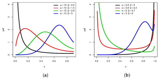
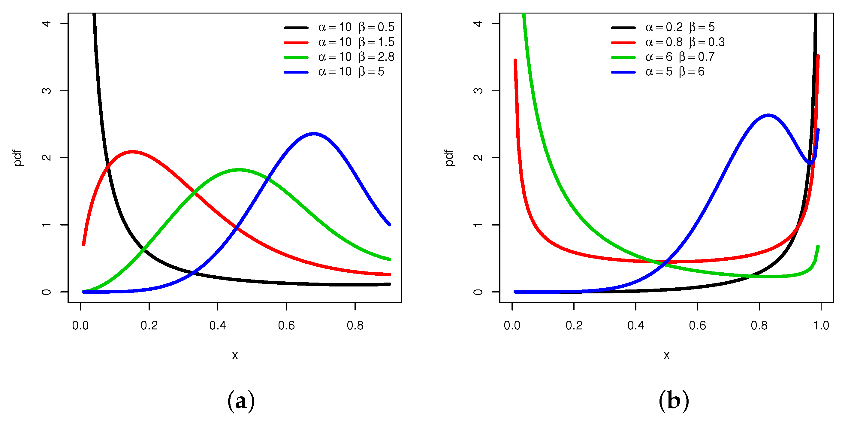
Figure 1. Plots showing different shapes of the pdf of the MKw distribution: (a) decreasing and unimodal shapes and (b) U- and N-shapes.

From Figure 1, we remark that $f_{MKw}(x;\alpha ,\beta )$ can be decreasing, unimodal with all the possible skewed directions, and also can be U- and N-shapes, which remains a rare property for a distribution supported on $(0,1)$. In particular, the almost angular monotonicity, “strongly” left-or right-skewed and N shape properties are not immediate for the Kw distribution. To this first graphical analysis, we propose to show the versatility of $f_{MKw}(x;\alpha ,\beta )$ via three-dimensional (3D) plots in Figure 2 and Figure 3, with moving $\alpha$ for Figure 2, and moving $\beta$ for Figure 3.

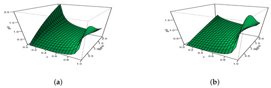
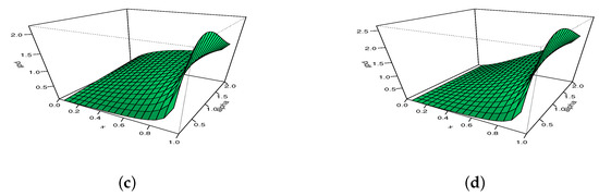
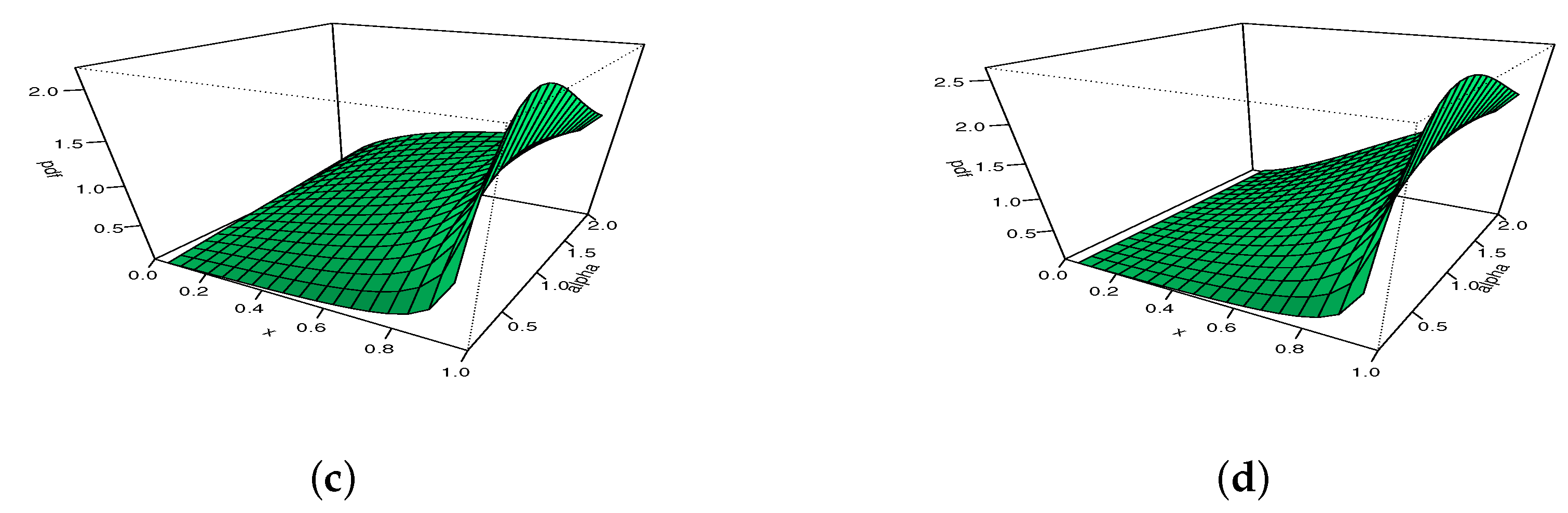
Figure 2. The 3D plots of the pdf of the MKw distribution for $\alpha \in \left[1,2\right]$ with (a) $\beta =0.5$, (b) $\beta =0.9$, (c) $\beta =1.5$, and (d) $\beta =2.5$.

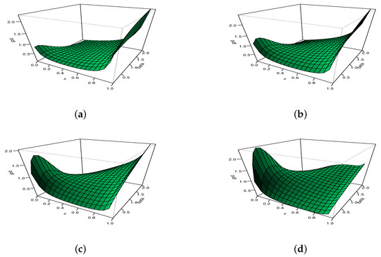
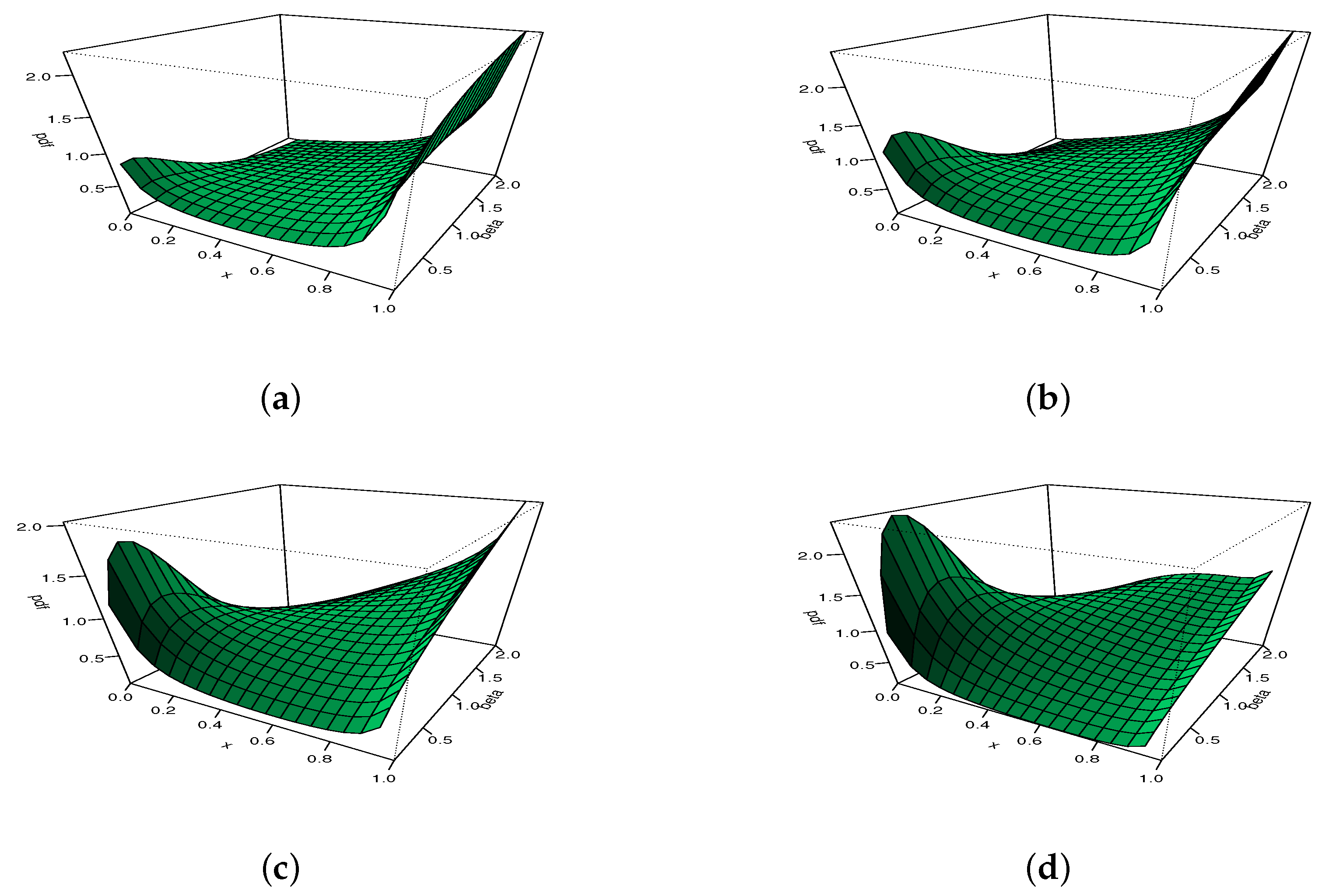
Figure 3. The 3D plots of the pdf of the MKw distribution for $\beta \in \left[1,2\right]$ with (a) $\alpha =0.5$, (b) $\alpha =0.9$, (c) $\alpha =1.5$, and (d) $\alpha =2.5$.

The hrf of the MKw distribution is given by the following:

$$\begin{array}{cc}\hfill h_{MKw}(x;\alpha ,\beta )& =\frac{f_{MKw}(x;\alpha ,\beta )}{1-F_{MKw}(x;\alpha ,\beta )}\hfill \\ \hfill & =\frac{\beta x^{\beta -1}\left[{(1-x^{\beta })}^{\alpha }(1-\alpha ln(1-x^{\beta }))-1\right]}{(x^{\beta }-1)ln(1-x^{\beta })[{(1-x^{\beta })}^{\alpha }-1]},x\in (0,1),\hfill \end{array}$$

and $h_{MKw}(x;\alpha ,\beta )=0$ for $x\notin (0,1)$. This function is difficult to explore using traditional mathematical tools, due to its analytical complexity. We proceed in the same manner as for $f_{MKw}(x;\alpha ,\beta )$. In the neighborhood of $x=0$, we have the following:

$$h_{MKw}(x;\alpha ,\beta )\sim \frac{\beta \alpha }{2}{x}^{\beta -1}.$$

As a result, $h_{MKw}(x;\alpha ,\beta )$ explodes to $+\infty$ for $\beta <1$ (and thus cannot be increasing), is equal to the constant $\alpha /2$ for $\beta =1$, and tends to 0 for $\beta >1$. The values of $\beta$ are thus of particular importance for the limit points. In the neighborhood of $x=1$, we obtain the following:

$$h_{MKw}(x;\alpha ,\beta )\sim -\beta \frac{1}{(1-x^{\beta })ln(1-x^{\beta })}.$$

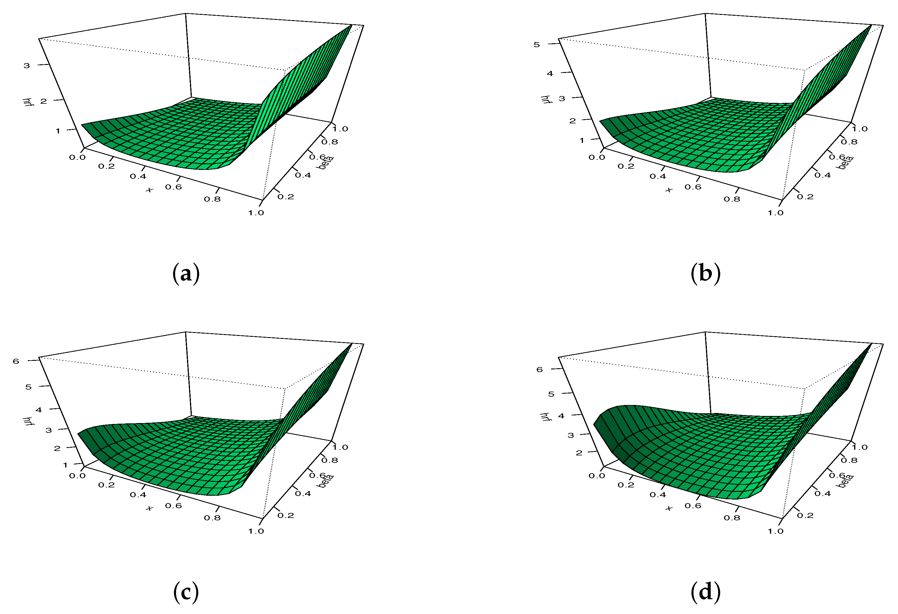
Hence, $h_{MKw}(x;\alpha ,\beta )$ exploses to $+\infty$ for all the values of $\alpha >0$ and $\beta >0$. A graphical analysis now completes these results, with a focus on the possible shapes of $h_{MKw}(x;\alpha ,\beta )$. The maximum number of distinct shapes of $h_{MKw}(x;\alpha ,\beta )$ can be seen in Figure 4.

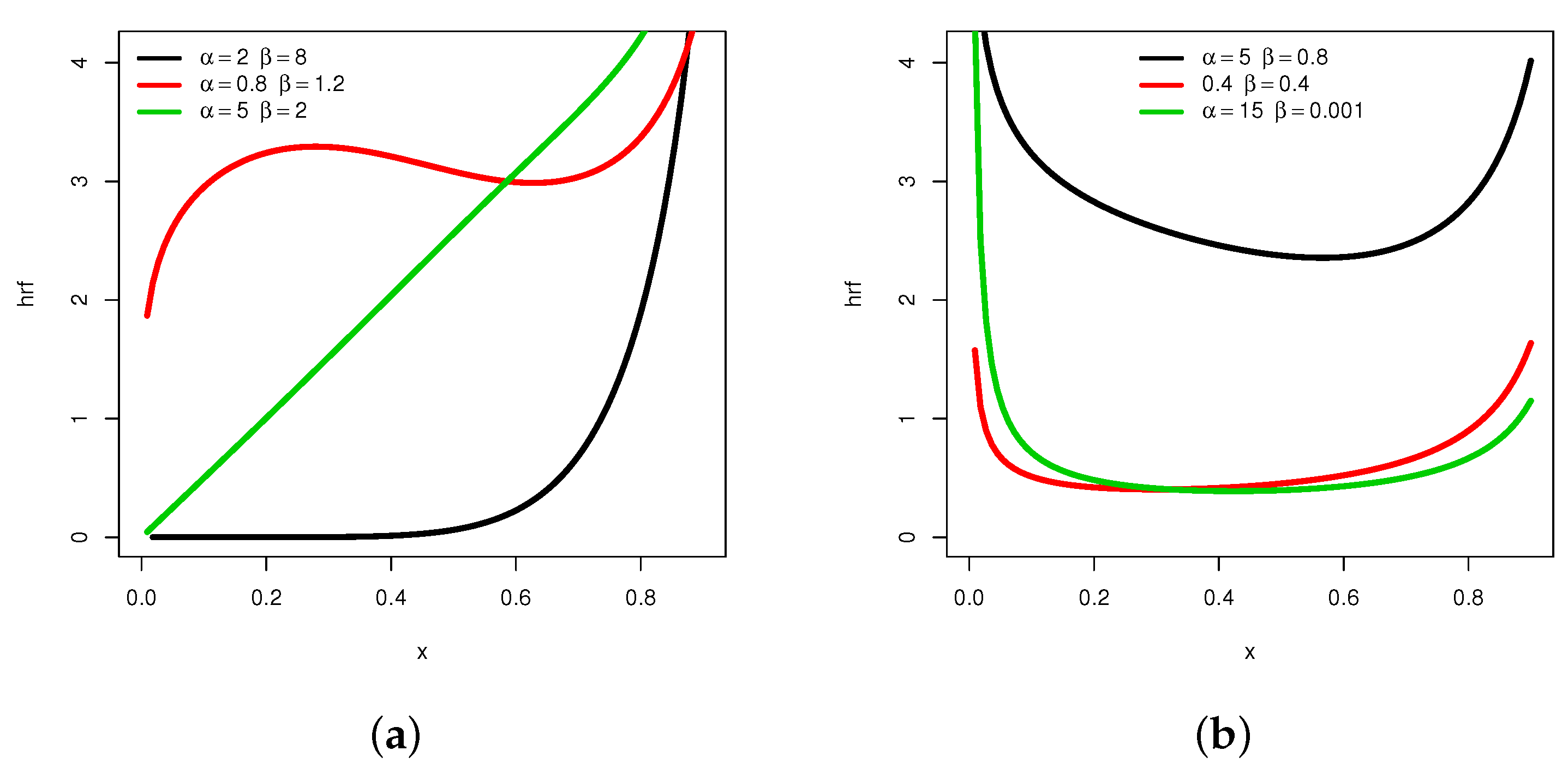
Figure 4. Plots showing different shapes of the hrf of the MKw distribution: (a) increasing, convex, constant and N-shapes, and (b) U-shapes.

From Figure 4, it is clear that $h_{MKw}(x;\alpha ,\beta )$ can be increasing with various convex properties, and can be non-monotonic with N- or U- shapes. Again, these remain as rare features for a distribution supported on $(0,1)$. For instance, the hrf of the Kw distribution does not possess an N shape.

To illustrate the adaptability of $h_{MKw}(x;\alpha ,\beta )$, we propose to use 3D plots in Figure 5 and Figure 6, with moving $\alpha$ for Figure 5 and moving $\beta$ for Figure 6.

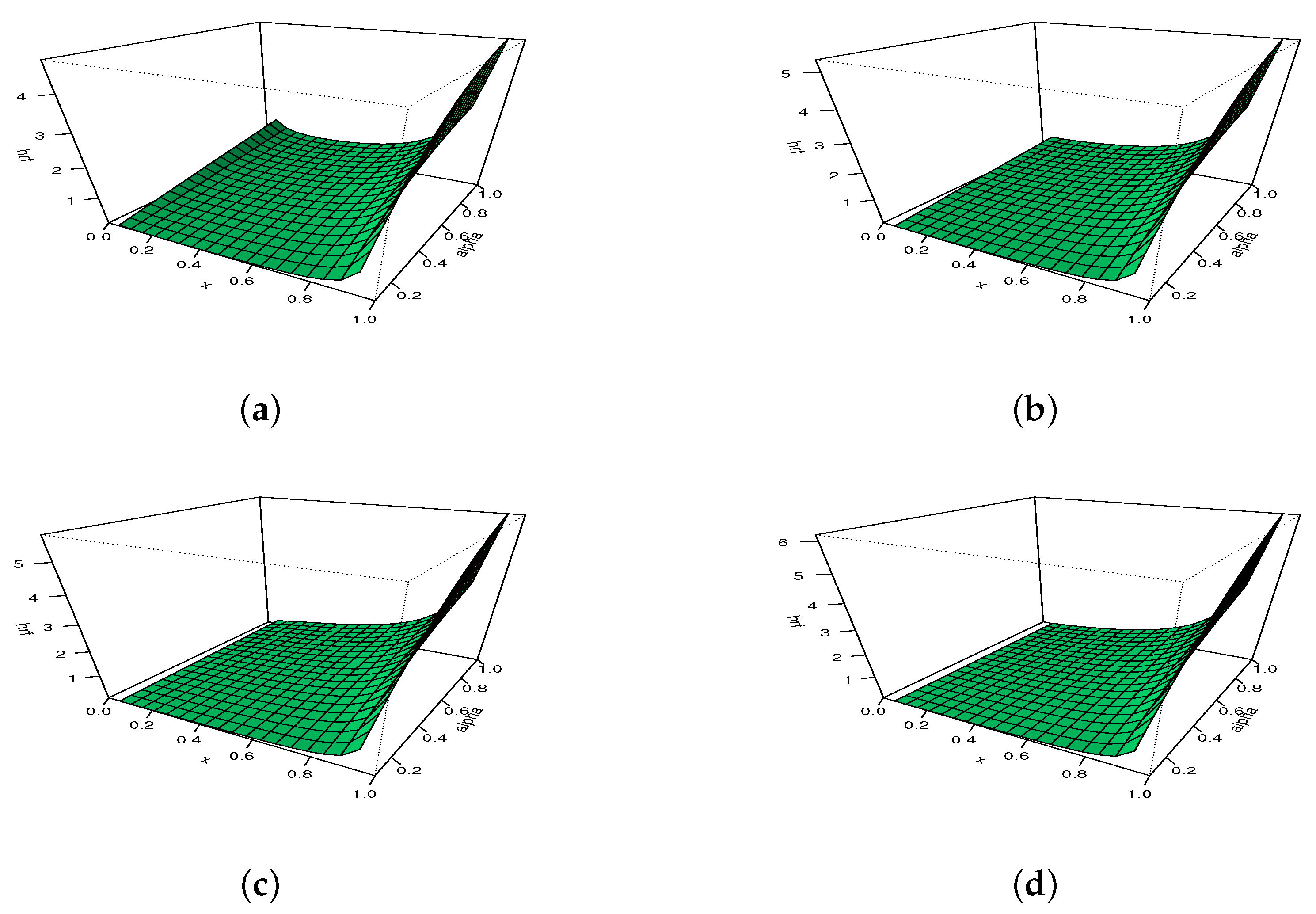
Figure 5. The 3D plots of the hrf of the MKw distribution for $\alpha \in \left[1,2\right]$ with (a) $\beta =0.5$, (b) $\beta =0.9$, (c) $\beta =1.5$, and (d) $\beta =2.5$.

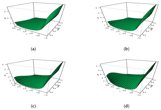
Figure 6. The 3D plots of the hrf of the MKw distribution for $\beta \in \left[1,2\right]$ with (a) $\alpha =0.5$, (b) $\alpha =0.9$, (c) $\alpha =1.5$, and (d) $\alpha =2.5$.

3. Mathematical Analysis

The MKw distribution is now mathematically treated, with emphasis on the quantile and moment features.

3.1. Quantile Analysis

The fact that the cdf of the KMw distribution is invertible is one of its most notable features. The quantile function (qf) can be expressed in closed form in terms of the principal branch of the Lambert function, as described in the next proposition. We may refer to [21] for further details on the Lambert function.

Proposition 2.

The qf of the MKw distribution is defined by the following:

$$Q_{MKw}(u;\alpha ,\beta )={\left[\alpha (1-u)W_0\left(-\frac{1}{\alpha (1-u)}{e}^{-1/\left[\alpha \right(1-u\left)\right]}\right)+1\right]}^{1/\beta },u\in (0,1),$$

where $W_0\left(x\right)$ denotes the principal branch of the Lambert function.

Proof. 

The qf is defined by $Q_{MKw}(u;\alpha ,\beta )=F_{MKw}^{-1}(u;\alpha ,\beta )$. Therefore, we can determine it by solving the following nonlinear equation: $F_{MKw}(y;\alpha ,\beta )=u$ with respect to y. We proceed as follows:

$$\begin{array}{cc}\hfill & u=F_{MKw}(y;\alpha ,\beta )\iff u=1-\frac{{(1-y^{\beta })}^{\alpha }-1}{\alpha ln(1-y^{\beta })}\iff \frac{{(1-y^{\beta })}^{\alpha }-1}{\alpha ln(1-y^{\beta })}=1-u\hfill \\ \hfill & \iff ln(1-y^{\beta })=\frac{{(1-y^{\beta })}^{\alpha }-1}{\alpha (1-u)}\iff 1-y^{\beta }=e^{{(1-y^{\beta })}^{\alpha }/\left[\alpha (1-u)\right]}{e}^{-1/\left[\alpha \right(1-u\left)\right]}\hfill \\ \hfill & \iff -\frac{1-y^{\beta }}{\alpha (1-u)}{e}^{-{(1-y^{\beta })}^{\alpha }/\left[\alpha (1-u)\right]}=-\frac{1}{\alpha (1-u)}{e}^{-1/\left[\alpha \right(1-u\left)\right]}\hfill \\ \hfill & \iff -\frac{1-y^{\beta }}{\alpha (1-u)}=W_0\left(-\frac{1}{\alpha (1-u)}{e}^{-1/\left[\alpha \right(1-u\left)\right]}\right)\hfill \\ \hfill & \iff y={\left[\alpha (1-u)W_0\left(-\frac{1}{\alpha (1-u)}{e}^{-1/\left[\alpha \right(1-u\left)\right]}\right)+1\right]}^{1/\beta }.\hfill \end{array}$$

We obtain the expected result. □

The expression of the qf is essential to determine the main quartle of the MKw distribution, such as the median defined by the following:

$$M=Q_{MKw}\left(\frac{1}{2};\alpha ,\beta \right)={\left[\frac{\alpha }{2}{W}_0\left(-\frac{2}{\alpha }{e}^{-2/\alpha }\right)+1\right]}^{1/\beta }.$$

Similarly, the first and third quartiles of the MKw distribution are given by $Q_1=Q_{MKw}(1/4;\alpha ,\beta )$ and $Q_3=Q_{MKw}(3/4;\alpha ,\beta )$. The octiles of the MKw distribution are given by $O_1=Q_{MKw}(1/8;\alpha ,\beta )$, $O_3=Q_{MKw}(3/8;\alpha ,\beta )$, $O_5=Q_{MKw}(5/8;\alpha ,\beta )$, and $O_7=Q_{MKw}(7/8;\alpha ,\beta )$. These special quantile values can serve as the main tool to describe the skewness and kurtosis of the distribution. For instance, we can measure the skewness via the quantile coefficient of Bowley defined by the following:

$$\mathrm{QS}=1-2\frac{M-Q_1}{Q_3-Q_1}.$$

On the other hand, we can measure the kurtosis by the quantile coefficient of Moors defined by the following:

$$\mathrm{QK}=\frac{O_7+O_3-(O_1+O_5)}{Q_3-Q_1}.$$

The sign of QS indicates the skewness of the MKw distribution: if $\mathrm{QS}>0$, the distribution is right-skewed; if $\mathrm{QS}<0$, the distribution is left-skewed; and if QS approaches 0, the distribution is nearly symmetric. Concerning the coefficient of Moors, we can compare it to the value of $1.233$, which corresponds to the quantile coefficient of Moors associated with the standard normal distribution. As a result, if $\mathrm{QK}<1.233$, the distribution is platykurtic; if $\mathrm{QK}>1.233$, the distribution is leptokurtic; and if QK approaches $1.233$, the distribution is mesokurtic.

The 3D plots for QS and QK for varying $\alpha$ and $\beta$ are displayed in Figure 7.

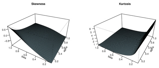
Figure 7. The 3D plots of QS and QK for $(\alpha ,\beta )\in {[0.1,1]}^2$.

From Figure 7, we see that the behavior of the quantile coefficients of skewness and kurtosis is consistent with what was determined in Figure 1, Figure 2 and Figure 3: the MKw distribution exhibits all sorts of skewness since QS might be positive, almost equal to 0, or positive. Furthermore, the fact that QK can be less than, nearly equal to, or larger than $1.2333$ demonstrates that all kurtosis levels are attained.

In addition, the expression of the qf is particularly useful for simulations. Indeed, pseudo-random data from the MKw distribution may be easily computer-generated using the inverse transform approach. Since the Lambert function is accessible in computer systems such as Maple, MATLAB and R, this approach is quite feasible. Further details on the above quantile analysis can be found in [22].

3.2. Moment Analysis

This section is devoted to the moment properties of the MKw distribution, beginning with the raw moments. Hereafter, we designate by X a random variable with the MKw distribution.

3.2.1. Raw Moments

For any integer r, the rth raw moment of X can be expressed in an integral form as follows:

$$\begin{array}{c}\hfill m\left(r\right)=E\left(X^r\right)={\int }_{-\infty }^{+\infty }{x}^r{f}_{MKw}(x;\alpha ,\beta )dx={\int }_0^1{x}^r\frac{\beta x^{\beta -1}\left[{(1-x^{\beta })}^{\alpha }(1-\alpha ln(1-x^{\beta }))-1\right]}{\alpha (x^{\beta }-1){[ln(1-x^{\beta })]}^2}dx.\end{array}$$

This integral can be implemented in any mathematical software, and can be calculated numerically for given values of $\alpha$ and $\beta$. Some mathematical developments of this integral are proposed in the next proposition.

Proposition 3.

Two representations of the rth moment of X are given below.

Representation 1.

We can express $m\left(r\right)$ in terms of the beta function as the following:

$$\begin{array}{c}\hfill m\left(r\right)=\frac{r}{\alpha \beta }{\int }_0^{\alpha }B\left(\frac{r}{\beta },t+1\right)dt,\end{array}$$

where $B(a,b)={\int }_0^1{t}^{a-1}{(1-t)}^{b-1}dt$, with $a>0$ and $b>0$.

Representation 2.

We can express $m\left(r\right)$ as the following series expansion:

$$\begin{array}{c}\hfill m\left(r\right)=1+\sum _{k=1}^{+\infty }\left(\genfrac{}{}{0pt}{}{r/\beta }{k}\right){(-1)}^k\left[1-\frac{k}{\alpha }ln\left(1+\frac{\alpha }{k}\right)\right].\end{array}$$

Proof. 

Let us prove the two representations in turn.

Representation 1.

First, by an integration by part, we have the following:

$$\begin{array}{c}\hfill m\left(r\right)=r{\int }_0^1{x}^{r-1}[1-F_{MKw}(x;\alpha ,\beta )]dx=r{\int }_0^1{x}^{r-1}\frac{{(1-x^{\beta })}^{\alpha }-1}{\alpha ln(1-x^{\beta })}dx=\frac{r}{\alpha }\psi (\alpha ,r),\end{array}$$

(4)

where

$$\begin{array}{c}\hfill \psi (\alpha ,r)={\int }_0^1{x}^{r-1}\frac{{(1-x^{\beta })}^{\alpha }-1}{ln(1-x^{\beta })}dx,\end{array}$$

with $\psi (\alpha ,r)=0$ for $\alpha =0$. Owing to the Leibnitz integral rule and the change of variables $y=x^{\beta }$, we have the following:

$$\begin{array}{cc}\hfill \frac{\partial }{\partial \alpha }\psi (\alpha ,r)& =\frac{\partial }{\partial \alpha }\left[{\int }_0^1{x}^{r-1}\frac{{(1-x^{\beta })}^{\alpha }-1}{ln(1-x^{\beta })}dx\right]={\int }_0^1{x}^{r-1}\frac{\partial }{\partial \alpha }\left[\frac{{(1-x^{\beta })}^{\alpha }-1}{ln(1-x^{\beta })}\right]dx\hfill \\ \hfill & ={\int }_0^1{x}^{r-1}{(1-x^{\beta })}^{\alpha }dx=\frac{1}{\beta }{\int }_0^1{y}^{r/\beta -1}{(1-y)}^{\alpha }dy=\frac{1}{\beta }B\left(\frac{r}{\beta },\alpha +1\right).\hfill \end{array}$$

Since $\psi (\alpha ,r)=0$ for $\alpha =0$, upon integration with respect to $\alpha$, we obtain the following:

$$\begin{array}{c}\hfill \psi (\alpha ,r)=\frac{1}{\beta }{\int }_0^{\alpha }B\left(\frac{r}{\beta },t+1\right)dt.\end{array}$$

(5)

The desired result follows by substituting Equation (5) in Equation (4).

Representation 2.

We recall that, in the distribution sense, X can be written as $X={(1-Y)}^{1/\beta }$, where Y follows the RPL distribution. Hence, for any positive integer r, the general binomial theorem yields the following infinite series representation:

$$\begin{array}{c}\hfill X^r=1+\sum _{k=1}^{+\infty }\left(\genfrac{}{}{0pt}{}{r/\beta }{k}\right){(-1)}^k{Y}^k.\end{array}$$

(6)

This expansion is valid almost everywhere; the event $\{Y=1\}$ is of probability zero. Now, let us present a known result (see [20] (Proposition 6)). We obviously have $E\left(Y^0\right)=1$, and, for any integer $k\ge 1$, the kth raw moment of Y is obtained as the following:

$$\begin{array}{c}\hfill m_{*}\left(k\right)=E\left(Y^k\right)=1-\frac{k}{\alpha }ln\left(1+\frac{\alpha }{k}\right).\end{array}$$

Therefore, based on Equation (6) and the linearity of the expectation operator, we have the following:

$$\begin{array}{cc}\hfill m\left(r\right)& =1+\sum _{k=1}^{+\infty }\left(\genfrac{}{}{0pt}{}{r/\beta }{k}\right){(-1)}^k{m}_{*}\left(k\right)\hfill \\ \hfill & =1+\sum _{k=1}^{+\infty }\left(\genfrac{}{}{0pt}{}{r/\beta }{k}\right){(-1)}^k\left[1-\frac{k}{\alpha }ln\left(1+\frac{\alpha }{k}\right)\right].\hfill \end{array}$$

The stated result is obtained.

The proof of Proposition 3 ends. □

By arranging the raw moments in a suitable manner, we can determine the standard central, dispersion, skewness, and kurtosis measures of X. These measures include the mean given by $m\left(1\right)$, the variance obtained through the Koenig–Huygens formula, $\mathrm{Var}=E({(X-m\left(1\right))}^2)=m\left(2\right)-{\left[m\left(1\right)\right]}^2$, the moment coefficient of skewness defined by

$$\begin{array}{c}\hfill \mathrm{MS}=\frac{1}{{\mathrm{Var}}^{3/2}}E\left({(X-m\left(1\right))}^3\right)=\frac{m\left(3\right)-3m\left(1\right)\mathrm{Var}-{\left[m\left(1\right)\right]}^3}{{\mathrm{Var}}^{3/2}},\end{array}$$

and the moment coefficient of kurtosis given by the following:

$$\begin{array}{c}\hfill \mathrm{MK}=\frac{1}{{\mathrm{Var}}^2}E\left({(X-m\left(1\right))}^4\right)=\frac{m\left(4\right)-4m\left(3\right)m\left(1\right)+6m\left(2\right){\left[m\left(1\right)\right]}^2-3{\left[m\left(1\right)\right]}^4}{{\mathrm{Var}}^2}.\end{array}$$

The interpretation of the moment skewness and kurtosis is similar to those of the quantile moment and kurtosis. The only difference is that, for the kurtosis, the benchmark value of the moment coefficient of kurtosis is 3 instead of $1.233$ for the quantile coefficient of kurtosis.

In addition, we can consider the coefficient of variation obtained as $\mathrm{CV}={\mathrm{Var}}^{1/2}/m\left(1\right)$ and the index of dispersion given as $\mathrm{ID}={\mathrm{Var}}^{1/2}\mathrm{CV}$. Table 1 shows the numerical values of $m\left(1\right)$, $m\left(2\right)$, $m\left(3\right)$, $m\left(4\right)$, Var, MS, MK, CV and ID for a random variable X following the MKw distribution with $\alpha =5$ and varying values of $\beta$, while Table 2 does the same with $\beta =3$ and varying $\alpha$.

Table 1. Numerical values of moment measures for a random variable X following the MKw distribution with $\alpha =5$ and varying $\beta$.

$\mathit{\beta }$	$\mathit{m}\left(1\right)$	$\mathit{m}\left(2\right)$	$\mathit{m}\left(3\right)$	$\mathit{m}\left(4\right)$	Var	MS	MK	CV	ID
0.5	0.894	0.835	0.793	0.76	0.036	−2.736	11.244	0.213	0.041
1.0	0.838	0.744	0.679	0.63	0.042	−1.796	6.393	0.245	0.05
1.5	0.798	0.676	0.602	0.545	0.039	−0.032	−6.622	0.248	0.049
2.0	0.762	0.631	0.543	0.477	0.05	−1.3	3.891	0.295	0.066
2.5	0.734	0.587	0.496	0.428	0.048	−0.534	−0.3	0.298	0.065
3.0	0.711	0.553	0.458	0.389	0.048	−0.419	0.127	0.309	0.068
3.5	0.69	0.525	0.424	0.357	0.049	−0.483	2.431	0.32	0.071
4.0	0.672	0.5	0.397	0.33	0.049	−0.38	2.341	0.329	0.073
4.5	0.655	0.478	0.374	0.308	0.049	−0.292	2.287	0.337	0.074

Table 2. Numerical values of moment measures for a random variable X following the MKw distribution with $\beta =3$ and varying $\alpha$.

$\mathit{\alpha }$	$\mathit{m}\left(1\right)$	$\mathit{m}\left(2\right)$	$\mathit{m}\left(3\right)$	$\mathit{m}\left(4\right)$	Var	MS	MK	CV	ID
0.5	0.213	0.129	0.101	0.087	0.084	1.574	4.215	1.357	0.393
1.0	0.354	0.213	0.156	0.129	0.087	0.729	2.727	0.834	0.247
1.5	0.459	0.288	0.211	0.172	0.077	0.387	2.428	0.604	0.168
2.0	0.537	0.354	0.264	0.211	0.066	0.133	2.036	0.48	0.124
2.5	0.595	0.411	0.311	0.251	0.057	−0.084	2.195	0.401	0.096
3.0	0.641	0.459	0.354	0.288	0.049	−0.215	2.258	0.345	0.076
3.5	0.677	0.501	0.393	0.323	0.042	−0.377	2.749	0.303	0.062
4.0	0.707	0.537	0.428	0.354	0.037	−0.503	2.951	0.272	0.052
4.5	0.732	0.568	0.459	0.384	0.032	−0.625	3.349	0.246	0.044

From both Table 1 and Table 2, we observe that the mean is monotonic with respect to $\alpha$ and $\beta$, which is not the case for the variance. Furthermore, wide variations of values are seen for the mean, whereas the variance remains relatively stable and small. The behavior of the moment coefficients of skewness and kurtosis are consistent with what is concluded in Figure 1, Figure 2 and Figure 3, as well as with the use of quantile coefficients of skewness and kurtosis; because MK can be positive, nearly equal to 0 or positive, the MKw distribution has all types of skewness. Moreover, since MK can be lower, almost equal or greater than 3, it indicates that all the kurtosis states are reached. In addition, we see a strong versatility in the numerical values of CV and ID.

All these comments are illustrated graphically in Figure 8 via 3D plots with varying $\alpha$ and $\beta$.

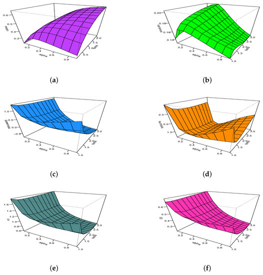
Figure 8. The 3D plots of the (a) mean, (b) variance, (c) moment skewness, (d) moment kurtosis, (e) coefficient of variation and (f) index of dispersion for the MKw distribution for $\alpha \in \left[0.1,0.9\right]$ and $\beta \in \left[1,3\right]$.

In the next part, we complete this moment analysis with the expression of the mean log moments, and the incomplete moments of X.

3.2.2. Other Kinds of Moments

The mean logarithm of X can be expressed in an integral form as follows:

$$\begin{array}{cc}\hfill m_{ln}& =E(ln\left(X\right))={\int }_{-\infty }^{+\infty }ln\left(x\right)f_{MKw}(x;\alpha ,\beta )dx\hfill \\ \hfill & ={\int }_0^{1}ln\left(x\right)\frac{\beta x^{\beta -1}\left[{(1-x^{\beta })}^{\alpha }(1-\alpha ln(1-x^{\beta }))-1\right]}{\alpha (x^{\beta }-1){[ln(1-x^{\beta })]}^2}dx.\hfill \end{array}$$

This kind of moment appears in some estimation methods, and entropy. It has the advantage of having values in $\mathbb{R}$, as opposed to $m\left(1\right)$, which has values in $(0,1)$. This can be of interest for the construction of regression models, among other things. The integral defining $m_{ln}$ may be determined numerically for given values of $\alpha$ and $\beta$ and can be implemented in any mathematical software. In the following result, the mean logarithm of X is stated as a series expansion.

Proposition 4.

The mean logarithm of X is the following:

$$\begin{array}{c}\hfill m_{ln}=\frac{1}{\beta }\sum _{k=1}^{+\infty }\frac{{(-1)}^{k-1}}{k}\left[1-\frac{k}{\alpha }ln\left(1+\frac{\alpha }{k}\right)\right].\end{array}$$

Proof. 

For this proof, we adopt the setting used in the proof of Representation 2 of Proposition 3. By using the relationship between the MKw and RPL distributions, and the logarithmic series expansion, we obtain the following:

$$\begin{array}{cc}\hfill m_{ln}& =\frac{1}{\beta }E(ln(1-Y))=\frac{1}{\beta }\sum _{k=1}^{+\infty }\frac{{(-1)}^{k-1}}{k}{m}_{*}\left(k\right)\hfill \\ \hfill & =\frac{1}{\beta }\sum _{k=1}^{+\infty }\frac{{(-1)}^{k-1}}{k}\left[1-\frac{k}{\alpha }ln\left(1+\frac{\alpha }{k}\right)\right].\hfill \end{array}$$

The desired expansion is proved. □

Now, let $y\in [0,1]$ and $X_y$ be the random variable equal to X if $X\le y$, and 0 otherwise. Then, the rth incomplete moment of X truncated at y can be expressed as the following:

$$\begin{array}{c}\hfill m\left(r\right)\left[y\right]=E\left(X_y^r\right)={\int }_{-\infty }^y{x}^r{f}_{MKw}(x;\alpha ,\beta )dx={\int }_0^y{x}^r\frac{\beta x^{\beta -1}\left[{(1-x^{\beta })}^{\alpha }(1-\alpha ln(1-x^{\beta }))-1\right]}{\alpha (x^{\beta }-1){[ln(1-x^{\beta })]}^2}dx.\end{array}$$

The incomplete moments are involved in a lot of probabilistic measures and functions, such as various mean deviations, residual life-type functions and curves. The integral defining $m\left(r\right)\left[y\right]$ may be determined numerically for given values of $\alpha$ and $\beta$ and can be implemented in any scientific software. The following proposition proposes a mathematical development of this integral.

Proposition 5.

Two representations of the rth incomplete moment of X truncated at y are given below.

Representation 1.

We can express $m\left(r\right)\left[y\right]$ in terms of the incomplete beta function as the following:

$$\begin{array}{c}\hfill m\left(r\right)\left[y\right]=-y^r\frac{{(1-y^{\beta })}^{\alpha }-1}{\alpha ln(1-y^{\beta })}+\frac{r}{\alpha \beta }{\int }_0^{\alpha }{B}_{y^{\beta }}\left(\frac{r}{\beta },t+1\right)dt,\end{array}$$

where $B_c(a,b)={\int }_0^c{t}^{a-1}{(1-t)}^{b-1}dt$, with $a>0$, $b>0$ and $c\in [0,1]$.

Representation 2.

We can express $m\left(r\right)\left[y\right]$ as the following series expansion:

$$\begin{array}{c}\hfill m\left(r\right)\left[y\right]=1+\sum _{k=1}^{+\infty }\left(\genfrac{}{}{0pt}{}{r/\beta }{k}\right){(-1)}^k\left[y^k\frac{y^{\alpha }-1}{ln\left(y\right)}-\frac{k}{\alpha }\left\{Ei\left[\right(\alpha +k)ln(y\left)\right]-Ei[kln(y\left)\right]\right\}\right],\end{array}$$

where $Ei\left(x\right)={\int }_{-\infty }^x{e}^t/tdt$, $x\in {\mathbb{R}}^{*}$.

Proof. 

Let us prove the two representations in turn.

Representation 1.

First, by an integration by part, we obtain the following:

$$\begin{array}{cc}\hfill m\left(r\right)\left[y\right]& =-y^r[1-F_{MKw}(y;\alpha ,\beta )]+r{\int }_0^y{x}^{r-1}[1-F_{MKw}(x;\alpha ,\beta )]dx\hfill \\ \hfill & =-y^r\frac{{(1-y^{\beta })}^{\alpha }-1}{\alpha ln(1-y^{\beta })}+r{\int }_0^y{x}^{r-1}\frac{{(1-x^{\beta })}^{\alpha }-1}{\alpha ln(1-x^{\beta })}dx\hfill \\ \hfill & =-y^r\frac{{(1-y^{\beta })}^{\alpha }-1}{\alpha ln(1-y^{\beta })}+\frac{r}{\alpha }\psi (\alpha ,r)\left[y\right],\hfill \end{array}$$

(7)

where

$$\begin{array}{c}\hfill \psi (\alpha ,r)\left[y\right]={\int }_0^y{x}^{r-1}\frac{{(1-x^{\beta })}^{\alpha }-1}{ln(1-x^{\beta })}dx,\end{array}$$

with $\psi (\alpha ,r)\left[y\right]=0$ for $\alpha =0$. By applying the Leibnitz integral rule and the change of variables $z=x^{\beta }$, we obtain the following:

$$\begin{array}{cc}\hfill \frac{\partial }{\partial \alpha }\psi (\alpha ,r)\left[y\right]& =\frac{\partial }{\partial \alpha }\left[{\int }_0^y{x}^{r-1}\frac{{(1-x^{\beta })}^{\alpha }-1}{ln(1-x^{\beta })}dx\right]={\int }_0^y{x}^{r-1}\frac{\partial }{\partial \alpha }\left[\frac{{(1-x^{\beta })}^{\alpha }-1}{ln(1-x^{\beta })}\right]dx\hfill \\ \hfill & ={\int }_0^y{x}^{r-1}{(1-x^{\beta })}^{\alpha }dx=\frac{1}{\beta }{\int }_0^{y^{\beta }}{z}^{r/\beta -1}{(1-z)}^{\alpha }dz=\frac{1}{\beta }{B}_{y^{\beta }}\left(\frac{r}{\beta },\alpha +1\right).\hfill \end{array}$$

Since $\psi (\alpha ,r)\left[y\right]=0$ for $\alpha =0$, upon integration with respect to $\alpha$, we obtain the following:

$$\begin{array}{c}\hfill \psi (\alpha ,r)\left[y\right]=\frac{1}{\beta }{\int }_0^{\alpha }{B}_{y^{\beta }}\left(\frac{r}{\beta },t+1\right)dt.\end{array}$$

(8)

Substituting Equation (8) in Equation (7) yields the desired result.

Representation 2.

To begin, let us introduce a known result (see [20] (Proposition 9)). The kth incomplete moment of a random variable Y with the RPL distribution at y with $y\in [0,1]$ is given by the following:

$$\begin{array}{c}\hfill m_{*}\left(k\right)\left[y\right]=y^k\frac{y^{\alpha }-1}{ln\left(y\right)}-\frac{k}{\alpha }\left\{Ei\left[\right(\alpha +k)ln(y\left)\right]-Ei[kln(y\left)\right]\right\}.\end{array}$$

Hence, by using Equation (6), we have the following:

$$\begin{array}{cc}\hfill m\left(r\right)\left[y\right]& =1+\sum _{k=1}^{+\infty }\left(\genfrac{}{}{0pt}{}{r/\beta }{k}\right){(-1)}^k{m}_{*}\left(k\right)\left[y\right]\hfill \\ \hfill & =1+\sum _{k=1}^{+\infty }\left(\genfrac{}{}{0pt}{}{r/\beta }{k}\right){(-1)}^k\left[y^k\frac{y^{\alpha }-1}{ln\left(y\right)}-\frac{k}{\alpha }\left\{Ei\left[\right(\alpha +k)ln(y\left)\right]-Ei[kln(y\left)\right]\right\}\right].\hfill \end{array}$$

The stated result is obtained.

The proof of Proposition 5 ends. □

The remainder of the work is devoted to the creation of a new data analysis paradigm based on the MKw model.

3.3. Order Statistics

In this section, we cover the fundamentals of the order statistics of the MKw distribution. Let n be a positive integer and $X_1,\cdots ,X_n$ be independent and identically distributed random variables following the MKw distribution. We consider the random variables $X_{1:n},\dots ,X_{n:n}$ defined as the ordered versions of $X_1,\cdots ,X_n$, such that $P(X_{1:n}\le \dots \le X_{n:n})=1$. Then, for any $j=1,2,\dots ,n$, the pdf of $X_{j:n}$ is given as the following:

$$\begin{array}{cc}\hfill f_{j:n}(x;\alpha ,\beta )& =\frac{n!}{(j-1)!(n-j)!}{f}_{MKw}(x;\alpha ,\beta ){\left[F_{MKw}(x;\alpha ,\beta )\right]}^{j-1}{[1-F_{MKw}(x;\alpha ,\beta )]}^{n-j}.\hfill \end{array}$$

That is, in an expanded form, we have the following:

$$\begin{array}{cc}\hfill f_{j:n}(x;\alpha ,\beta )& =\frac{n!}{(j-1)!(n-j)!}\frac{\beta x^{\beta -1}\left[{(1-x^{\beta })}^{\alpha }(1-\alpha ln(1-x^{\beta }))-1\right]}{\alpha (x^{\beta }-1){[ln(1-x^{\beta })]}^2}\times \hfill \\ \hfill & {\left[1-\frac{{(1-x^{\beta })}^{\alpha }-1}{\alpha ln(1-x^{\beta })}\right]}^{j-1}{\left[\frac{{(1-x^{\beta })}^{\alpha }-1}{\alpha ln(1-x^{\beta })}\right]}^{n-j},x\in (0,1),\hfill \end{array}$$

and $f_{j:n}(x;\alpha ,\beta )=0$ for $x\notin (0,1)$. In particular, if we focus on the two extreme order statistics, the pdf of $X_{1:n}$ is given by

$$\begin{array}{cc}\hfill f_{1:n}(x;\alpha ,\beta )& =n\frac{\beta x^{\beta -1}\left[{(1-x^{\beta })}^{\alpha }(1-\alpha ln(1-x^{\beta }))-1\right]}{\alpha (x^{\beta }-1){[ln(1-x^{\beta })]}^2}{\left[\frac{{(1-x^{\beta })}^{\alpha }-1}{\alpha ln(1-x^{\beta })}\right]}^{n-1},x\in (0,1),\hfill \end{array}$$

and $f_{1:n}(x;\alpha ,\beta )=0$ for $x\notin (0,1)$, and the pdf of $X_{n:n}$ is given by the following:

$$\begin{array}{cc}\hfill f_{n:n}(x;\alpha ,\beta )& =n\frac{\beta x^{\beta -1}\left[{(1-x^{\beta })}^{\alpha }(1-\alpha ln(1-x^{\beta }))-1\right]}{\alpha (x^{\beta }-1){[ln(1-x^{\beta })]}^2}{\left[1-\frac{{(1-x^{\beta })}^{\alpha }-1}{\alpha ln(1-x^{\beta })}\right]}^{n-1},x\in (0,1),\hfill \end{array}$$

and $f_{n:n}(x;\alpha ,\beta )=0$ for $x\notin (0,1)$. Moment analysis is possible using these formulas. However, due to the functional complexity of the pdfs, numerical evaluations appear to necessitate the employment of computer mathematical tools.

4. Statistical Inference

The parameters $\alpha$ and $\beta$ of the MKw distribution are now considered to be unknown and must be calculated using data. As a result, the MKw model is examined.

4.1. Estimation Method

The maximum likelihood (MLL) technique is well adapted for this purpose. The specifics of this estimation strategy are outlined below.

Let $x_1,x_2,\dots ,x_n$ symbolize the n values lying into $(0,1)$ that are predicted to be seen from a random variable X with the MKw distribution and unknown parameters $\alpha$ and $\beta$. Then, the log-likelihood function for $\alpha$ and $\beta$ is formulated as the following:

$$\begin{array}{cc}\hfill \mathfrak{L}(\alpha ,\beta )& =\sum _{i=1}^{n}ln\left[f_{MKw}(x_i;\alpha ,\beta )\right]\hfill \\ \hfill & =nln\beta -nln\alpha +(\beta -1)\sum _{i=1}^{n}ln\left(x_i\right)-\sum _{i=1}^{n}ln(1-x_i^{\beta })-2\sum _{i=1}^{n}ln\left[-ln(1-{x_i}^{\beta })\right]\hfill \\ \hfill & +\sum _{i=1}^{n}ln\left[1-{\left(1-{x_i}^{\beta }\right)}^{\alpha }\left(1-\alpha ln\left(1-{x_i}^{\beta }\right)\right)\right].\hfill \end{array}$$

The MLL estimates (MLLEs) of $\alpha$ and $\beta$, denoted by $\widehat{\alpha }$ and $\widehat{\beta }$, are defined by the following:

$$(\widehat{\alpha },\widehat{\beta })={argmax}_{(\alpha ,\beta )\in {(0,+\infty )}^2}\mathfrak{L}(\alpha ,\beta ).$$

These MLLEs fulfill the partial derivative equations listed below: $\partial \mathfrak{L}(\alpha ,\beta )/\partial \alpha =0$, and $\partial \mathfrak{L}(\alpha ,\beta )/\partial \beta =0$, where

$$\begin{array}{c}\hfill \frac{\partial \mathfrak{L}(\alpha ,\beta )}{\partial \alpha }=-\frac{n}{\alpha }+\sum _{i=1}^n\frac{z_i^{\alpha }\left\{ln\left(z_i\right)\left(1-\alpha ln\left(z_i\right)\right)+ln\left(z_i\right)\right\}}{z_i^{\alpha }\left(1-\alpha ln\left(z_i\right)\right)-1}\end{array}$$

and

$$\begin{array}{c}\hfill \frac{\partial \mathfrak{L}(\alpha ,\beta )}{\partial \beta }=\frac{n}{\beta }+\sum _{i=1}^{n}ln\left(x_i\right)+\sum _{i=1}^n\frac{t_i}{z_i}+2\sum _{i=1}^n\frac{t_i}{z_{i}ln\left(z_i\right)}+{\alpha }^2\sum _{i=1}^n\frac{z_i^{\alpha -1}{t}_{i}ln\left(z_i\right)}{z_i^{\alpha }\left(1-\alpha ln\left(z_i\right)\right)-1},\end{array}$$

where $z_i=1-{x_i}^{\beta }$ and $t_i={x_i}^{\beta }ln\left(x_i\right)$. Due to the intricacy of these partial derivatives, it is difficult to derive closed-form equations for $\widehat{\alpha }$ and $\widehat{\beta }$. Computational methods can be used to obtain precise numerical solutions. With the MMLEs, we can estimate all the functions of the MKw model by insertion. In particular, $f_{MKw}(x;\alpha ,\beta )$ and $F_{MKw}(x;\alpha ,\beta )$ may be naturally estimated by $f_{MKw}(x;\widehat{\alpha },\widehat{\beta })$ and $F_{MKw}(x;\widehat{\alpha },\widehat{\beta })$, respectively.

A two-dimensional normal distribution with the mean $(\alpha ,\beta )$ and matrix of covariance could be used to identify the asymptotic distribution of the random version of $(\widehat{\alpha },\widehat{\beta })$. To be more specific, the matrix of covariance is given by $\mathfrak{D}=I{(\alpha ,\beta )}^{-1}{\mid }_{(\alpha ,\beta )=(\widehat{\alpha },\widehat{\beta })}$, where the following holds:

$$\begin{array}{c}\hfill I(\alpha ,\beta )=-\left(\begin{array}{cc}{\displaystyle \frac{{\partial }^2\mathfrak{L}(\alpha ,\beta )}{\partial {\alpha }^2}}& {\displaystyle \frac{{\partial }^2\mathfrak{L}(\alpha ,\beta )}{\partial \alpha \partial \beta }}\\ .& {\displaystyle \frac{{\partial }^2\mathfrak{L}(\alpha ,\beta )}{\partial {\beta }^2}}\end{array}\right).\end{array}$$

The matrix $\mathfrak{D}$ can be computed quantitatively using mathematical techniques. We can establish estimated confidence intervals (CoIs) for $\alpha$ and $\beta$ at a particular level, such as $100(1-q)\%$ with $q\in (0,1)$. The associated lower bounds (CoI-LBs) and upper bounds (CoI-UBs) of such intervals remain traditional; if we keep our eyes on the unknown parameter $\alpha$, these interval bounds are provided by CoI-LB $=\widehat{\alpha }-z_q{\mathrm{SEr}}_{\alpha }$ and CoI-UB $=\widehat{\alpha }+z_q{\mathrm{SEr}}_{\alpha }$, where $z_q$ is defined by $P\left(\right|Z|\ge z_q)=q$, with Z a random variable having the standard Gaussian distribution, and ${\mathrm{SEr}}_{\alpha }$ is a term that relates to the standard error (SEr) of $\widehat{\alpha }$, determined by the square root of the first diagonal element of $\mathfrak{D}$. For more theoretical and practical achievements of the MLLEs, see [23].

4.2. Simulation

Here, we perform simulation work to measure the behavior of the constructed MLLEs. In this situation, we employ the R program, which was created by [24]. The following steps are taken into consideration:

• We apply the inverse transform approach to produce 10,000 random samples with values $x_1,x_2,\dots ,x_n$. That is, for any $i=1,\dots ,n$, the value $x_i$ is computed as $x_i=Q_{MKw}(u_i;\alpha ,\beta )$, where $u_i$ is a value generated from the uniform distribution on $(0,1)$.
• Six different sample sizes are taken into account: $n=30$, 50, 100, 200, 500, and 1000.
• Throughout the vector of parameters $(\alpha ,\beta )$, we consider seven possible configurations.
• For the examined configurations, the average MLLEs, mean square errors (MSErs), CoI-LBs, CoI-UBs, and length (CoI-LEN) of the CoIs are computed at two distinct levels (90% and 95%).
• Table 3, Table 4, Table 5, Table 6, Table 7, Table 8 and Table 9 show the outcomes that were achieved.
  Table 3. Numerical values of the MLLEs, MSErs, CoI-LBs, CoI-UBs, and CoI-LENs for ($\alpha$ = 0.5, $\beta$ = 0.5) of the MKw model.

  n	MLLE	MSEr	90%			95%
  			CoI-LB	CoI-UB	CoI-LEN	CoI-LB	CoI-UB	CoI-LEN
  30	1.6622	0.3629	0.9792	2.3451	1.3659	0.8485	2.4759	1.6274
  	0.5311	0.0223	0.3457	0.7165	0.3708	0.3102	0.7520	0.4418
  50	1.6082	0.1195	1.1166	2.0998	0.9833	1.0224	2.1940	1.1716
  	0.5268	0.0111	0.3848	0.6688	0.2840	0.3576	0.6960	0.3384
  100	1.5114	0.0382	1.1943	1.8284	0.6341	1.1336	1.8891	0.7555
  	0.4998	0.0037	0.4037	0.5958	0.1922	0.3853	0.6142	0.2290
  200	1.5141	0.0180	1.2896	1.7386	0.4490	1.2466	1.7816	0.5350
  	0.5015	0.0018	0.4333	0.5697	0.1364	0.4203	0.5828	0.1625
  500	1.4992	0.0060	1.3593	1.6392	0.2799	1.3325	1.6660	0.3335
  	0.4991	0.0006	0.4561	0.5421	0.0860	0.4479	0.5503	0.1024
  1000	1.5151	0.0039	1.4146	1.6155	0.2009	1.3954	1.6348	0.2394
  	0.5042	0.0004	0.4735	0.5348	0.0613	0.4677	0.5407	0.0731

  Table 4. Numerical values of the MLLEs, MSErs, CoI-LBs, CoI-UBs, and CoI-LENs for ($\alpha$ = 0.5, $\beta$ = 1.2) of the MKw model.

  n	MLLE	MSEr	90%			95%
  			CoI-LB	CoI-UB	CoI-LEN	CoI-LB	CoI-UB	CoI-LEN
  30	0.5485	0.0109	0.3935	0.7034	0.3099	0.3639	0.7331	0.3692
  	1.3745	0.1687	0.7487	2.0004	1.2517	0.6288	2.1202	1.4914
  50	0.5303	0.0073	0.4167	0.6439	0.2273	0.3949	0.6657	0.2708
  	1.3645	0.1538	0.8800	1.8489	0.9690	0.7872	1.9417	1.1545
  100	0.5125	0.0023	0.4354	0.5896	0.1541	0.4207	0.6043	0.1836
  	1.2505	0.0428	0.9322	1.5687	0.6365	0.8713	1.6297	0.7583
  200	0.5038	0.0011	0.4508	0.5569	0.1062	0.4406	0.5671	0.1265
  	1.2282	0.0216	1.0060	1.4504	0.4444	0.9634	1.4929	0.5295
  500	0.4973	0.0005	0.4644	0.5302	0.0658	0.4581	0.5365	0.0784
  	1.1947	0.0099	1.0575	1.3319	0.2744	1.0313	1.3582	0.3269
  1000	0.4999	0.0002	0.4765	0.5233	0.0469	0.4720	0.5278	0.0558
  	1.2039	0.0027	1.1062	1.3015	0.1953	1.0875	1.3202	0.2326

  Table 5. Numerical values of the MLLEs, MSErs, CoI-LBs, CoI-UBs, and CoI-LENs for ($\alpha$ = 1.2, $\beta$ = 0.5) of the MKw model.

  n	MLLE	MSEr	90%			95%
  			CoI-LB	CoI-UB	CoI-LEN	CoI-LB	CoI-UB	CoI-LEN
  30	1.2612	0.0859	0.8003	1.7221	0.9218	0.7120	1.8104	1.0983
  	0.4939	0.0137	0.3132	0.6746	0.3613	0.2786	0.7092	0.4305
  50	1.2505	0.0858	0.8961	1.6048	0.7087	0.8283	1.6727	0.8444
  	0.5147	0.0131	0.3683	0.6610	0.2927	0.3403	0.6891	0.3487
  100	1.2547	0.0323	1.0054	1.5041	0.4987	0.9577	1.5518	0.5941
  	0.5182	0.0049	0.4143	0.6222	0.2079	0.3944	0.6421	0.2477
  200	1.2206	0.0099	1.0516	1.3896	0.3380	1.0192	1.4219	0.4028
  	0.5035	0.0014	0.4318	0.5752	0.1433	0.4181	0.5889	0.1708
  500	1.2091	0.0050	1.1037	1.3145	0.2107	1.0835	1.3346	0.2511
  	0.5035	0.0007	0.4581	0.5489	0.0908	0.4494	0.5576	0.1082
  1000	1.2081	0.0015	1.1338	1.2824	0.1486	1.1196	1.2967	0.1771
  	0.5055	0.0004	0.4733	0.5377	0.0644	0.4671	0.5439	0.0768

  Table 6. Numerical values of the MLLEs, MSErs, CoI-LBs, CoI-UBs, and CoI-LENs for ($\alpha$ = 0.8, $\beta$ = 0.5) of the MKw model.

  n	MLLE	MSEr	90%			95%
  			CoI-LB	CoI-UB	CoI-LEN	CoI-LB	CoI-UB	CoI-LEN
  30	0.8409	0.0326	0.5709	1.1109	0.5400	0.5192	1.1626	0.6434
  	0.5234	0.0217	0.3126	0.7342	0.4216	0.2722	0.7746	0.5024
  50	0.8634	0.0248	0.6475	1.0793	0.4318	0.6062	1.1206	0.5144
  	0.5526	0.0157	0.3816	0.7235	0.3419	0.3489	0.7562	0.4073
  100	0.8432	0.0083	0.6963	0.9901	0.2938	0.6681	1.0182	0.3501
  	0.5268	0.0048	0.4109	0.6428	0.2319	0.3887	0.6650	0.2764
  200	0.8118	0.0024	0.7046	0.8989	0.1943	0.6860	0.9175	0.2315
  	0.5074	0.0016	0.4273	0.5875	0.1601	0.4120	0.6028	0.1908
  500	0.8038	0.0020	0.7559	0.8817	0.1258	0.7439	0.8938	0.1499
  	0.5098	0.0015	0.4593	0.5603	0.1010	0.4496	0.5699	0.1203
  1000	0.8023	0.0009	0.7589	0.8456	0.0867	0.7506	0.8539	0.1033
  	0.5011	0.0004	0.4658	0.5363	0.0706	0.4590	0.5431	0.0841

  Table 7. Numerical values of the MLLEs, MSErs, CoI-LBs, CoI-UBs, and CoI-LENs for ($\alpha$ = 0.8, $\beta$ = 0.8) of the MKw model.

  n	MLLE	MSEr	90%			95%
  			CoI-LB	CoI-UB	CoI-LEN	CoI-LB	CoI-UB	CoI-LEN
  30	0.8875	0.0505	0.5967	1.1783	0.5815	0.5411	1.2340	0.6929
  	0.8732	0.0513	0.5263	1.2201	0.6939	0.4598	1.2866	0.8268
  50	0.8615	0.0244	0.6491	1.0739	0.4248	0.6084	1.1146	0.5062
  	0.8514	0.0345	0.5889	1.1139	0.5250	0.5386	1.1642	0.6255
  100	0.8282	0.0114	0.6837	0.9726	0.2888	0.6561	1.0002	0.3441
  	0.8408	0.0162	0.6545	1.0271	0.3726	0.6188	1.0628	0.4440
  200	0.8035	0.0028	0.7063	0.9007	0.1943	0.6877	0.9193	0.2316
  	0.8069	0.0056	0.6798	0.9340	0.2541	0.6555	0.9583	0.3028
  500	0.8040	0.0014	0.7426	0.8653	0.1227	0.7309	0.8771	0.1462
  	0.8033	0.0021	0.7233	0.8832	0.1599	0.7080	0.8985	0.1905
  1000	0.7977	0.0006	0.7547	0.8407	0.0860	0.7465	0.8489	0.1024
  	0.8008	0.0011	0.7443	0.8573	0.1130	0.7335	0.8681	0.1346

  Table 8. Numerical values of the MLLEs, MSErs, CoI-LBs, CoI-UBs, and CoI-LENs for ($\alpha$ = 0.5, $\beta$ = 1.5) of the MKw model.

  n	MLLE	MSEr	90%			95%
  			CoI-LB	CoI-UB	CoI-LEN	CoI-LB	CoI-UB	CoI-LEN
  30	0.5295	0.0103	0.3812	0.6777	0.2965	0.3529	0.7061	0.3532
  	1.7019	0.3967	0.9201	2.4837	1.5636	0.7704	2.6334	1.8630
  50	0.5269	0.0061	0.4128	0.6410	0.2282	0.3909	0.6628	0.2719
  	1.6688	0.1760	1.0730	2.2646	1.1916	0.9589	2.3786	1.4197
  100	0.5192	0.0026	0.4411	0.5973	0.1562	0.4262	0.6123	0.1861
  	1.5894	0.0557	1.1863	1.9925	0.8063	1.1091	2.0697	0.9606
  200	0.5065	0.0010	0.4531	0.5600	0.1068	0.4429	0.5702	0.1273
  	1.5332	0.0327	1.2565	1.8100	0.5535	1.2035	1.8630	0.6595
  500	0.5006	0.0004	0.4674	0.5339	0.0665	0.4610	0.5403	0.0792
  	1.5192	0.0115	1.3450	1.6934	0.3484	1.3116	1.7267	0.4151
  1000	0.4998	0.0002	0.4764	0.5233	0.0469	0.4719	0.5278	0.0559
  	1.5007	0.0057	1.3790	1.6224	0.2434	1.3557	1.6457	0.2900

  Table 9. Numerical values of the MLLEs, MSErs, CoI-LBs, CoI-UBs, and CoI-LENs for ($\alpha$ = 0.5, $\beta$ = 2.0) of the MKw model.

  n	MLLE	MSEr	90%			95%
  			CoI-LB	CoI-UB	CoI-LEN	CoI-LB	CoI-UB	CoI-LEN
  30	0.5206	0.0063	0.3754	0.6658	0.2904	0.3476	0.6936	0.3460
  	2.1889	0.3108	1.1732	3.2046	2.0313	0.9788	3.3991	2.4203
  50	0.5237	0.0043	0.4117	0.6357	0.2239	0.3903	0.6571	0.2668
  	2.1641	0.2081	1.3904	2.9377	1.5474	1.2422	3.0859	1.8437
  100	0.5095	0.0021	0.4334	0.5857	0.1524	0.4188	0.6003	0.1816
  	2.0274	0.1227	1.5102	2.5447	1.0345	1.4111	2.6437	1.2326
  200	0.4988	0.0009	0.4464	0.5512	0.1048	0.4364	0.5612	0.1248
  	2.0031	0.0449	1.6395	2.3667	0.7272	1.5699	2.4363	0.8664
  500	0.5019	0.0003	0.4685	0.5353	0.0668	0.4621	0.5417	0.0796
  	1.9800	0.0214	1.7531	2.2070	0.4538	1.7097	2.2504	0.5407
  1000	0.5014	0.0002	0.4778	0.5250	0.0472	0.4733	0.5296	0.0563
  	1.9914	0.0072	1.8299	2.1529	0.3230	1.7990	2.1838	0.3849

From the tables above, we see that the values of MLLEs are near to the values of the parameters provided in the settings as n rises. Furthermore, when n rises, the MSEr and CoI-LEN values fall, as one would anticipate.

5. Application

It is critical to demonstrate how the MKw model may be used in practice. This is the aim of this section.

5.1. Method

In the coming applications, the fits of the MKw model are compared with those of some competitive models, such as the transmuted Kumaraswamy (TKw), Kumaraswamy (Kw), beta (B), unit Rayleigh (UR), Topp–Leone (Topp), and Power models. The TKw model has three parameters, whereas the other models have two parameters only. These models are defined through their cdfs in Table 10.

Table 10. Competent models with the MKw model.

Models	Cdfs	References
TKw	${\displaystyle [1-{(1-x^{\alpha })}^{\theta }][1+\lambda {(1-x^{\alpha })}^{\theta }]}$	[6]
Kw	${\displaystyle 1-{(1-x^{\lambda })}^{\theta }}$	[4]
Beta	${\displaystyle \frac{1}{B({\alpha }_1,{\alpha }_2)}{\int }_0^x{t}^{{\alpha }_1-1}{(1-t)}^{{\alpha }_2-1}dt}$	[1]
UR	${\displaystyle e^{-\tau {[ln\left(x\right)]}^2}}$	[12]
Topp	${\displaystyle {\left[x(2-x)\right]}^{\mu }}$	[25]
Power	${\displaystyle x^{\nu }}$	(Classic)

In order to compare these models, we consider well-referenced statistical measures, namely the Cramér–Von Mises (W), Anderson–Darling (A), Kolmogorov–Smirnov (KS), and Akaike information criterion (AIC) based on the minus maximal likelihood value, denoted by $-\widehat{\ell }$. The best model is the one with the smallest values of these statistics and criteria. We refer to [26] for more information on the usage and underlying meaning of the measures W, A, KS and AIC. In addition, we extract the p-value associated with the KS test. The best model is the one with the largest p-value.

As for the simulated part, the results are obtained using the R software, and two real data sets are considered.

5.2. Maximum Flood Level Data Set

The first data set comes from [27] and contains environmental data. It refers to 20 observations of the Susquehanna River’s greatest flood level (measured in millions of cubic feet per second) in Harrisburg, Pennsylvania. The data are 0.26, 0.27, 0.30, 0.32, 0.32, 0.34, 0.38, 0.38, 0.39, 0.40, 0.41, 0.42, 0.42, 0.42, 0.45, 0.48, 0.49, 0.61, 0.65, 0.74. A histogram analysis reveals that the data are unimodal and right skewed, with a small left-skewed tail. Theoretically, in view of the shape ability of the related pdf, the MKw model is able to fit these data.

Following our methodology, we first determine the MLLEs and the related SEs of the considered models in Table 11.

Table 11. MLLEs and SEs of the models for the maximum flood level data set.

Models		MLLEs (SEs)
MKw	354.0108	5.9002
$(\alpha ,\beta )$	(5.0365)	(1.2035)
TKw	3.7445	11.1649	0.6201
$(\alpha ,\theta ,\lambda )$	(0.6505)	(6.1634)	(0.3722)
Kw	3.3773	12.0018
$(\lambda ,\theta )$	(0.6041)	(5.4713)
Beta	6.8309	9.2364
$({\alpha }_1,{\alpha }_2)$	(2.1179)	(2.8912)
UR	1.1366
$\left(\tau \right)$	(0.2541)
Topp	2.2412
$\left(\mu \right)$	(0.5011)
Power	1.7804
$\left(\nu \right)$	(0.2487)

From Table 11, if we focus on the MKw model, we see that $\widehat{\alpha }=354.0108$ and $\widehat{\beta }=5.9002$. By using these estimates, we derive function estimates for the pdf and cdf of the MKw model through the substitution method; $f_{MKw}(x;\alpha ,\beta )$ and $F_{MKw}(x;\alpha ,\beta )$ may be naturally estimated by $f_{MKw}(x;\widehat{\alpha },\widehat{\beta })$ and $F_{MKw}(x;\widehat{\alpha },\widehat{\beta })$, respectively.

The models are compared via our statistical benchmarks in Table 12.

Table 12. Values of $-\widehat{\ell }$, AIC, W, A, KS and (KS p-value) of the models for the maximum flood level data set.

Models	$-\widehat{\mathit{\ell }}$	AIC	W	A	KS	p-Value
MKw	−15.7652	−27.5305	0.0437	0.2959	0.1143	0.9562
TKw	−13.6401	−21.2802	0.1420	0.8417	0.2001	0.3993
Kw	−12.9732	−21.9465	0.1672	0.9746	0.2175	0.3004
Beta	−14.18350	−24.3671	0.1267	0.7514	0.2062	0.3625
UR	−11.1176	−20.2352	0.0892	0.5367	0.2892	0.0704
Topp	−7.3813	−12.7627	0.1194	0.7110	0.3409	0.0191
Power	−0.1097	1.7804	0.1229	0.7300	0.3977	0.0035

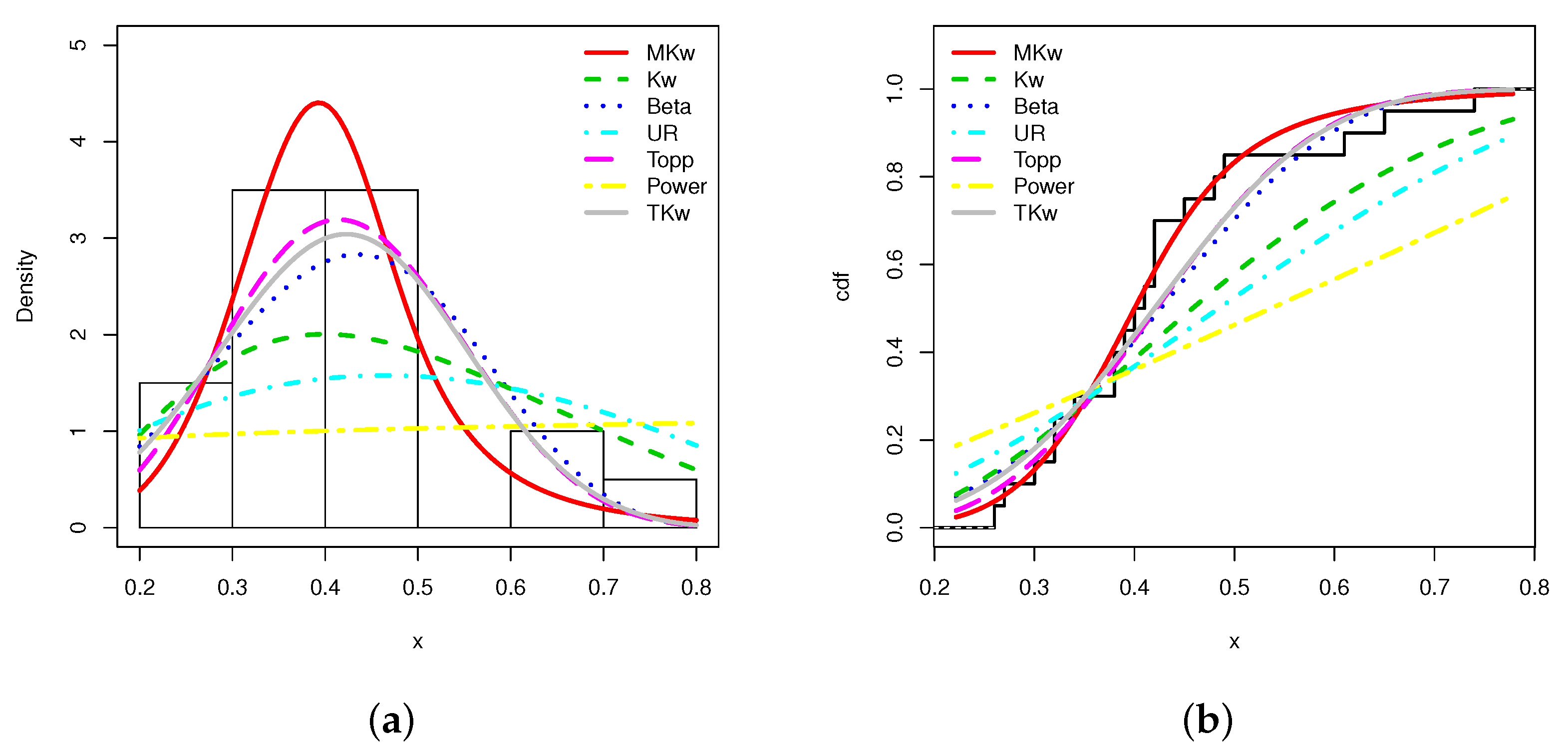
From Table 12, it is clear that the MKw model is the best, followed by the TKw model. Indeed, the MKw model has the smallest AIC, W, A, KS, and the largest p-values among all the considered models. We illustrate this claim through a graphical approach. Figure 9 plots the estimated pdfs and cdfs over the appropriate empirical objects.

Figure 9. Plots of the (a) estimated pdfs and (b) estimated cdfs over the appropriate statistical objects for the maximum flood level data set.

Based on Figure 9, we see that the fits of the MKw model are the best; the estimated pdf has well captured the form of the histogram, and well detected the lack of observations over the interval $[0.5,0.6]$. Furthermore, the estimated cdf is very close to the scale shape of the empirical cdf.

5.3. Air Conditioning System Data Set

The second data set involves the failure times of an airplane’s air cooling system (in hours), as reported by [28]. The data are 23, 261, 87, 7, 120, 14, 62, 47, 225, 71, 246, 21, 42, 20, 5, 12, 120, 11, 3, 14, 71, 11, 14, 11, 16, 90, 1, 16, 52, 95. We perform a normalization operation on these data by dividing them by 265 to obtain data between 0 and 1. To put it another way, we work with the following data: 0.086792453, 0.984905660, 0.328301887, 0.026415094, 0.452830189, 0.052830189, 0.233962264, 0.177358491, 0.849056604, 0.267924528, 0.928301887, 0.079245283, 0.158490566, 0.075471698, 0.018867925, 0.045283019, 0.452830189, 0.041509434, 0.011320755, 0.052830189, 0.267924528, 0.041509434, 0.052830189, 0.041509434, 0.060377358, 0.339622642, 0.003773585, 0.060377358, 0.196226415, 0.358490566. A histogram analysis reveals that the data are decreasing and right skewed, with some data close to 1 that need to be considered. The MKw model can theoretically fit these data due to the shape ability of the corresponding pdf. Recently, these data were taken into account in [12] to illustrate the applicability of the UR model. By proceeding in the same way for the maximum flood level data set, we show that the MKw model is more appropriate for these data.

First, we determine the MLLEs and the related SEs of the considered models in Table 13.

Table 13. MLLEs and SEs of the models for the air conditioning system data set.

Models	MLLEs (SEs)
MKw	11.6229	0.9719
$(\alpha ,\beta )$	(1.8815)	(0.1868)
TKw	0.6274	1.1217	0.6622
$(\alpha ,\theta ,\lambda )$	(0.1245)	(0.3444)	(0.2631)
Kw	0.5451	1.3837
$(\lambda ,\theta )$	(0.1148)	(0.3361)
Beta	0.5141	1.3429
$({\alpha }_1,{\alpha }_2)$	(0.1118)	(0.3642)
UR	0.1497
$\left(\tau \right)$	(0.0273)
Topp	0.6017
$\left(\mu \right)$	(0.1098)
Power	0.4501
$\left(\nu \right)$	(0.0821)

Table 13 shows that $\widehat{\alpha }=11.6229$ and $\widehat{\beta }=0.9719$ are the MLLEs for the MKw model. By using these estimates, we obtain the estimated pdf and cdf of the MKw model through the substitution method.

Table 14 gives the necessary values to compare the models.

Table 14. Values of $-\widehat{\ell }$, AIC, W, A, KS and (KS p-value) of the models for the air conditioning system data set.

Models	$-\widehat{\mathit{\ell }}$	AIC	W	A	KS	p-Value
MKw	−17.8873	−31.7747	0.0929	0.4899	0.1261	0.7260
TKw	−14.9975	−23.9950	0.1691	1.0856	0.1744	0.3210
Kw	−13.5389	−23.0778	0.2109	1.3470	0.1878	0.2403
Beta	−13.2463	−22.49261	0.2173	1.3858	0.1957	0.2003
UR	−12.7730	−23.5461	0.1253	0.7933	0.1314	0.6776
Topp	−11.9801	−21.9603	0.2379	1.5102	0.1938	0.2095
Power	−12.7018	−23.4036	0.2068	1.3212	0.2031	0.1680

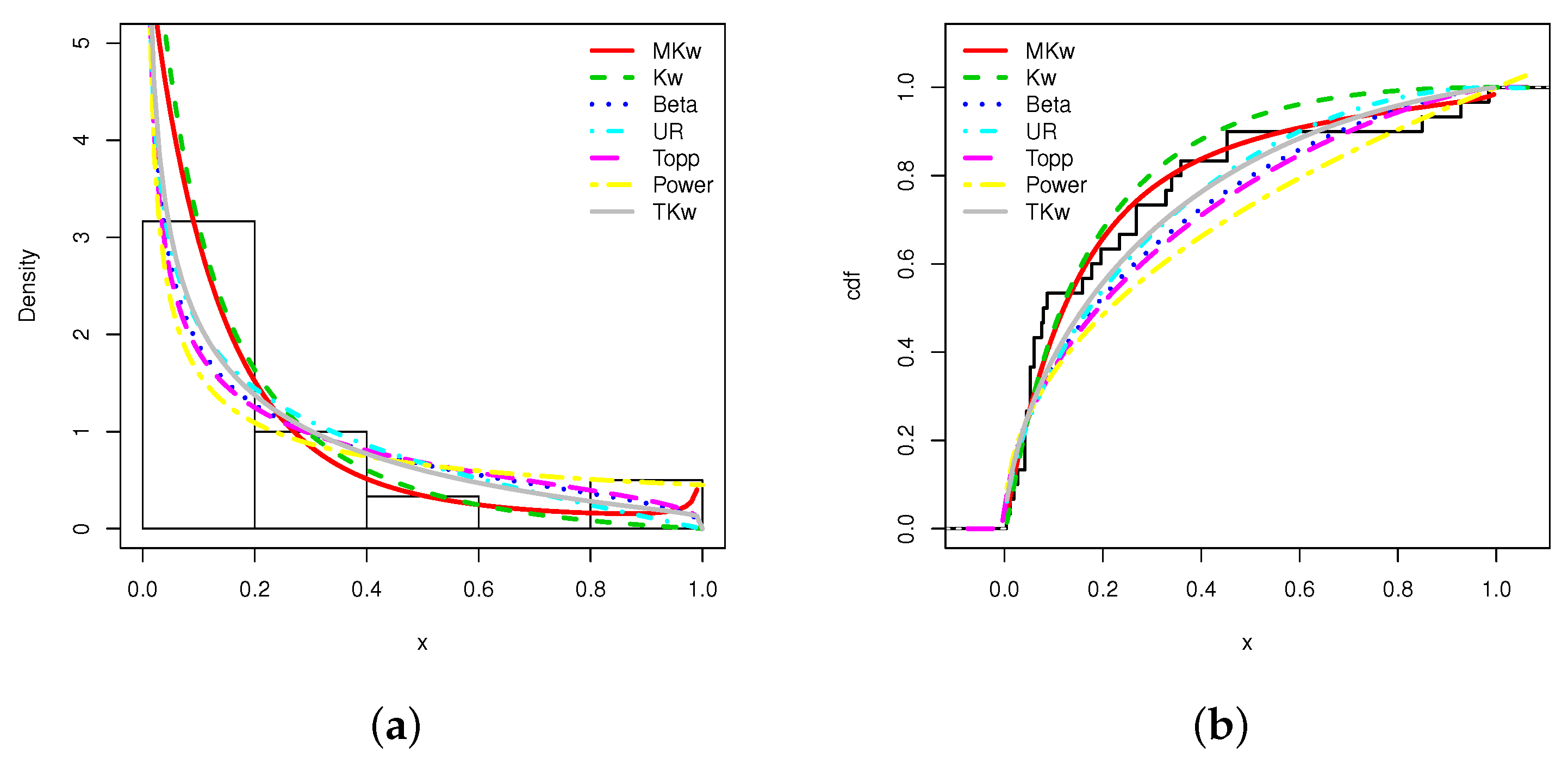
Table 14 clearly shows that the MKw model is the best; it has the more desirable AIC, W, A, KS, and p-values of all the models studied. We use a graphical way to demonstrate this assertion. The estimated pdfs and cdfs are plotted over the corresponding empirical objects in Figure 10.

Figure 10. Plots of the (a) estimated pdfs and (b) estimated cdfs over the appropriate statistical objects for the air conditioning system data set.

According to Figure 10, the MKw model fits best; the predicted pdf captures the form of the histogram quite well and has taken into account the values close to 1, contrary to the other models. Furthermore, the scale shape of the empirical cdf is extremely similar to the scale shape of the estimated cdf.

6. Conclusions

In this paper, a new distribution modifying the functional capabilities and mathematical structure of the Kumaraswamy distribution is proposed. We have called it the modified Kumaraswamy distribution. Evidence shows that it is more efficient than the Kumaraswamy distribution for the modeling of phenomena with data presenting a histogram that is monotonic in a nearly angular way, “strongly” left- or right-skewed, and of a leptokurtic nature, or N-shaped. On the stochastic plan, the modified Kumaraswamy distribution first order stochastic dominates the Kumaraswamy distribution. It is also deeply connected with the so-called ratio power-logarithmic distribution. In the first part, we have exhibited its main quantile and moment properties, with mathematical results, numerical tables, and graphics. These elements have offered the necessary comprehension of the distribution for further theoretical and practical purposes. In the statistical plan, an inferential methodology of the related model is developed. Then, two different data sets are analyzed with the proposed model, and other models of references: the Kumaraswamy, beta, unit Rayleigh, Topp–Leone and power models. The results are quite favorable to our modeling strategy. This study is thus encouraging for the use of the modified Kumaraswamy model for other statistical applications of importance in fields in full expansion, such as medicine, finance, biology, and environmental sciences. The development of likelihood inferential methods that take into account censored data, extensions to the multivariate case, incorporation of time series, spatial, and quantile regression structures in the modeling, and the development of influence diagnostic tools are some future research directions.

References

- Gupta, P.L.; Gupta, R.C. The monotonicity of the reliability measures of the beta distribution. Appl. Math. Lett. 2000, 13, 5–9. [Google Scholar] [CrossRef] [Green Version]
- Ghitany, M.E. The monotonicity of the reliability measures of the beta distribution. Appl. Math. Lett. 2004, 17, 1277–1283. [Google Scholar] [CrossRef]
- Ferrari, S.L.; Cribari-Neto, F. Beta regression for modelling rates and proportions. J. Appl. Stat. 2004, 31, 799–815. [Google Scholar] [CrossRef]
- Kumaraswamy, P. A generalized probability density function for double-bounded random processes. J. Hydrol. 1980, 46, 79–88. [Google Scholar] [CrossRef]
- Jones, M.C. Kumaraswamy’s distribution: A beta-type distribution with some tractability advantages. Stat. Methodol. 2009, 6, 70–81. [Google Scholar] [CrossRef]
- Khan, M.S.; King, R.; Hudson, I. Transmuted Kumaraswamy distribution. Stat. Transit. New Ser. 2016, 17, 1–28. [Google Scholar]
- Sharma, D.; Chakrabarty, T. On Size Biased Kumaraswamy Distribution. Statistics. Optim. Inf. Comput. 2016, 4, 252–264. [Google Scholar]
- Altun, E.; Hamedani, G.G. The log-xgamma distribution with inference and application. J. Soc. Fr. Stat. 2018, 159, 40–55. [Google Scholar]
- Mazucheli, J.; Menezes, A.F.; Dey, S. Unit-Gompertz distribution with applications. Statistica 2019, 79, 25–43. [Google Scholar]
- Gündüz, S.; Korkmaz, M.Ç. A new unit distribution based on the unbounded Johnson distribution rule: The unit Johnson SU distribution. Pak. J. Stat. Oper. Res. 2020, 16, 471–490. [Google Scholar] [CrossRef]
- Altun, E. The log-weighted exponential regression model: Alternative to the beta regression model. Commun. Stat.-Theory Methods 2020, 50, 2306–2321. [Google Scholar] [CrossRef]
- Bantan, R.A.R.; Chesneau, C.; Jamal, F.; Elgarhy, M.; Tahir, M.H.; Aqib, A.; Zubair, M.; Anam, S. Some new facts about the unit-Rayleigh distribution with applications. Mathematics 2020, 8, 1954. [Google Scholar] [CrossRef]
- Haq, M.A.; Hashmi, S.; Aidi, K.; Ramos, P.L.; Louzada, F. Unit modified Burr-III distribution: Estimation, characterizations and validation test. Ann. Data Sci. 2020. [Google Scholar] [CrossRef]
- Korkmaz, M.Ç.; Chesneau, C.; Korkmaz, Z.S. On the arcsecant hyperbolic normal distribution. Properties, quantile regression modeling and applications. Symmetry 2021, 13, 117. [Google Scholar] [CrossRef]
- Korkmaz, M.Ç.; Chesneau, C. On the unit Burr-XII distribution with the quantile regression modeling and applications. Comput. Appl. Math. 2021, 40, 1–26. [Google Scholar] [CrossRef]
- Chesneau, C. A note on an extreme left skewed unit distribution: Theory, modelling and data fitting. Open Stat. 2021, 2, 1–23. [Google Scholar] [CrossRef]
- Korkmaz, M.Ç.; Chesneau, C.; Korkmaz, Z.S. Transmuted unit Rayleigh quantile regression model: Alternative to beta and Kumaraswamy quantile regression models. Univ. Politeh. Buchar. Sci. Bull.-Ser. A-Appl. Math. Phys. 2021, 83, 149–158. [Google Scholar]
- Figueroa-Zu, J.I.; Niklitschek-Soto, S.A.; Leiva, V.; Liu, S. Modeling heavy-tailed bounded data by the trapezoidal beta distribution with applications. REVSTAT-Stat. J. 2021. Revstat, to appear. Available online: https://www.ine.pt/revstat/pdf/ModelingBoundedDataWithHeavyTails.pdf (accessed on 4 November 2021).
- Bakouch, H.S.; Nik, A.S.; Asgharzadeh, A.; Salinas, H.S. A flexible probability model for proportion data: Unit-half-normal distribution, Communications in Statistics-Case Studies. Data Anal. Appl. 2021. [Google Scholar] [CrossRef]
- Chesneau, C. Study of a unit power-logarithmic distribution. Open J. Math. Sci. 2021, 5, 218–235. [Google Scholar] [CrossRef]
- Corless, R.M.; Gonnet, G.H.; Hare, D.E.G.; Jeffrey, D.J.; Knuth, D.E. On the Lambert W function. Adv. Comput. Math. 1996, 5, 329–359. [Google Scholar] [CrossRef]
- Gilchrist, W. Statistical Modelling with Quantile Functions; CRC Press: Abingdon, UK, 2000. [Google Scholar]
- Casella, G.; Berger, R.L. Statistical Inference; Brooks/Cole Publishing Company: Bel Air, CA, USA, 1990. [Google Scholar]
- R Core Team. R: A Language and Environment for Statistical Computing; R Foundation for Statistical Computing: Vienna, Austria, 2013. [Google Scholar]
- Topp, C.W.; Leone, F.C. A family of J-shaped frequency functions. J. Am. Stat. Assoc. 1955, 50, 209–219. [Google Scholar] [CrossRef]
- Konishi, S.; Kitagawa, G. Information Criteria and Statistical Modeling; Springer: New York, NY, USA, 2007. [Google Scholar]
- Dumonceaux, R.; Antle, C.E. Discrimination between the Log-Normal and the Weibull distributions. Technometrics 1973, 15, 923–926. [Google Scholar] [CrossRef]
- Linhart, H.; Zucchini, W. Model Selection; Wiley: New York, NY, USA, 1986. [Google Scholar]
Publisher’s Note: MDPI stays neutral with regard to jurisdictional claims in published maps and institutional affiliations. |
© 2021 by the authors. Licensee MDPI, Basel, Switzerland. This article is an open access article distributed under the terms and conditions of the Creative Commons Attribution (CC BY) license (https://creativecommons.org/licenses/by/4.0/).