Stability Analysis of SEIRS Epidemic Model with Nonlinear Incidence Rate Function

Abstract

This paper addresses the global stability analysis of the SEIRS epidemic model with a nonlinear incidence rate function according to the Lyapunov functions and Volterra-Lyapunov matrices. By creating special conditions and using the properties of Volterra-Lyapunov matrices, it is possible to recognize the stability of the endemic equilibrium ($E_1$) for the SEIRS model. Numerical results are used to verify the presented analysis.

1. Introduction

The global stability of epidemiological models plays an imperative part in additionally foreseeing the advancement of the infection for embracing a methodology to control the disease [1,2,3,4]. Recently, the global stability of the endemic equilibrium has received impressive consideration and a few procedures have been discussed [5,6,7,8,9,10].

Incidence rates play a critical part in the mathematical modeling of diseases [11,12,13,14]. The bilinear rate is frequently utilized in many classical epidemiological models. In any case, because of the huge number of susceptible people, it is preposterous to consider a bilinear rate. Moreover, when the number of effective contacts between infective people and susceptible people may immerse at high infective levels, the rate may end up being nonlinear [15,16,17,18,19]. Suppose that $S\left(t\right),E\left(t\right),I\left(t\right)$, and $R\left(t\right)$ indicate the divisions of the population that are susceptible, exposed, infectious, and recovered, respectively, at time $t.$ As said sometime recently, a few models use the bilinear rate $\beta SI,$ where $\beta >0,$ but Liu et al. [15] proposed a rate of $\beta I^p{S}^q,$ where $p,q>0$. One common nonlinear incidence rate utilized in [20] is given by $\frac{\beta SI}{1+aI}$, where a is a nonnegative constant. We should note that a common incidence rate of $\beta Sf\left(I\right)$, where $f\left(0\right)=0, f\left(I\right)$ is positive for $0<I\left(t\right)<1$ and $f\in C^1(0,1],$ for all these epidemiological models makes a coordinates treatment conceivable [21]. Li et al. and Zheng et al. [12,20,22] investigated the dynamical behavior of an SEIRS epidemic model with a nonlinear incidence rate and assessed the stability analysis for the system’s equilibria.

Zheng et al. [20] solved the open problem for the bilinear case and reduced the constraint on general nonlinear transmission functions for the global stability. Within the present work, we consider the global stability of the endemic equilibrium of the SEIRS model with a nonlinear incidence rate. We use the combination of Lyapunov functions with the theory of Volterra-Lyapunov stable matrices [23,24,25,26]. Liao and Wang [23] pointed out the classical Lyapunov method with the aid of Volterra-Lyapunov stable matrices and demonstrated the global stability of the endemic equilibria. Tian and Wang [27] presented the global stability analysis for several deterministic cholera epidemic models. They used some approaches including the main method used in the present paper. This strategy can overcome the difficulty of determining specific coefficient values and, as such, a wider application of Lyapunov functions to dynamical systems could be promoted. A key point in the proposed method is its direct computational implementation. The method of Volterra-Lyapunov stable matrices [23] is modified using two Lemmas to overcome the problems of the standard technique [25].

The structure of this article is as follows. Section 2 presents the model formulation. Section 3 addresses the global stability of the endemic equilibrium. Section 4 demonstrates the effectiveness of the proposed method by means of numerical examples. Finally, Section 5 summarizes the results.

2. Model Formulation

Let us consider the SEIRS epidemic model with a common nonlinear incidence rate, $\beta Sf\left(I\right)$. We divide the population in four time-dependent classes, namely the fractions of the population that are susceptible $S\left(t\right),$ exposed $E\left(t\right),$ infected $I\left(t\right),$ and removed with immunity $R\left(t\right)$ [12]. This model is known as SEIRS because susceptibles become successively exposed, infected, removed, and susceptible again after the temporary immunity is lost. Additionally, assume that $S+E+I+R=1.$

The mathematical model of the SEIRS model is formulated by the following system of differential equations:

$$\begin{array}{c}\frac{dS}{dt}=\nu -\beta Sf\left(I\right)-\nu S+\delta R,\hfill \\ \frac{dE}{dt}=\beta Sf\left(I\right)-(ϵ+\nu )E,\hfill \\ \frac{dI}{dt}=ϵE-(\gamma +\nu )I,\hfill \\ \frac{dR}{dt}=\gamma I-(\delta +\nu )R.\hfill \end{array}$$

(1)

In order to describe the model, the parameters and assumptions are stated in Table 1.

Table 1. Description of the parameters.

Parameter	Description
$ϵ$	Rate of conversion of exposed population to infectious
$\gamma$	Rate of conversion of infectious to recovered
$\delta$	Rate of conversion of immunity to recovered
$\nu$	The birth (and death) rate
$f\left(I\right)$	The nonlinear transmission rate

In recent years, various types of incidence have been advanced, such as the bilinear incidence rate $\beta IS$ and the nonlinear incidence $\beta I^p{S}^q,$ where p and q are positive parameters. The classical bilinear incidence has $f\left(I\right)=I$ with $\beta$ for the constant contact rate. Hereafter, we adopt the nonlinear incidence $\beta Sf\left(I\right)=\frac{\beta SI}{1+aI},$ where a is a positive constant.

Equilibria of the Model

The goal of this part is to find the equilibrium points of the system (1). Let us introduce the disease-free equilibrium $E_0$

$$\begin{array}{c}\hfill E_0=\left(1,0,0,0\right).\end{array}$$

Further, the endemic equilibrium (if it exists) is calculated by

$$\begin{array}{c}\hfill E_1=\left(S_e,E_e,I_e,R_e\right),\end{array}$$

where $E_1$ satisfies the following equilibrium equations:

$$\begin{array}{c}\nu -\beta S_e\frac{I_e}{1+a{I}_e}-\nu S_e+\delta R_e=0,\hfill \end{array}$$

(2)

$$\begin{array}{c}\beta S_e\frac{I_e}{1+a{I}_e}-(ϵ+\nu )E_e=0,\hfill \end{array}$$

(3)

$$\begin{array}{c}ϵE_e-(\gamma +\nu )I_e=0,\hfill \end{array}$$

(4)

$$\begin{array}{c}\gamma I_e-(\delta +\nu )R_e=0.\hfill \end{array}$$

(5)

By adding Equations (2) and (3) and rewriting (3) and (5), we obtain:

$$\begin{array}{c}{S}_e=\frac{\nu +\delta R_e-(ϵ+\nu )E_e}{\nu },\hfill \\ E_e=\frac{\nu +\gamma }{ϵ}{I}_e,\hfill \\ R_e=\frac{\gamma }{\nu +\delta }{I}_e.\hfill \end{array}$$

From Equation (3), one concludes that system (2)–(5) has a nontrivial solution if the following equation has a positive solution $I_e\in (0,1)$

$$\begin{array}{c}\hfill \left(1-\frac{(ϵ+\nu )(\gamma +\nu )(\delta +\nu )-\gamma \delta ϵ}{\nu ϵ(\delta +\nu )}{I}_e\right)\times \frac{I_e}{(1+a{I}_e)}-\frac{(ϵ+\nu )(\gamma +\nu )I_e}{\beta ϵ}=0.\end{array}$$

(6)

In [12,20], some analyses on this model were conducted. Utilizing the next-generation matrix method [28], the basic reproductive rate can be calculated as

$$\begin{array}{c}\hfill R_0=\frac{ϵ\beta f^{\prime }\left(0\right)}{(ϵ+\nu )(\gamma +\nu )}.\end{array}$$

If $f\left(I\right)=\frac{I}{1+aI}$, then $f^{\prime }\left(0\right)=1$, and we have

$$\begin{array}{c}\hfill R_0=\frac{ϵ\beta }{(ϵ+\nu )(\gamma +\nu )}.\end{array}$$

3. Stability Analysis of the Endemic Equilibria

3.1. Notations

This section focuses on the stability analysis of $E_1$. The following definitions and notations are the requirements of this process.

Notation 1.

If the matrix M is symmetric positive (negative) definite, we shall write for simplicity $M>0$ (<0).

Definition 1.

[29] Suppose that the diagonal matrix $M_{n\times n}>0$ is so that $MC+C^T{M}^T<0$; then $C_{n\times n}$ is Volterra-Lyapunov stable.

Definition 2.

[29] Suppose that diagonal matrix $M_{n\times n}>0$ is so that $MC+C^T{M}^T>0$ then $C_{n\times n}$ is diagonally stable.

Proposition 1.

[29,30] The matrix $C=\left[\begin{array}{cc}{c}_{11}& c_{12}\\ c_{21}& c_{22}\end{array}\right]$ is Volterra-Lyapunov stable if, and only if:

$$\begin{array}{c}\hfill \left\{\begin{array}{c}{c}_{11}<0,\hfill \\ c_{22}<0,\hfill \\ det\left(C\right)=c_{11}{c}_{22}-c_{12}{c}_{21}>0.\hfill \end{array}\right.\end{array}$$

Proposition 2.

[31,32] Consider the nonsingular matrix $C_{n\times n}=\left[c_{ij}\right], (n\ge 2),$ the positive diagonal matrix $B_{n\times n}=diag(b_1,\cdots ,b_n)$ and $M=C^{-1}$, such that:

$$\begin{array}{c}\hfill \left\{\begin{array}{c}{c}_{nn}>0,\hfill \\ \tilde{B}\tilde{C}+{\left(\tilde{B}\tilde{C}\right)}^T>0,\hfill \\ \tilde{B}\tilde{M}+{\left(\tilde{B}\tilde{M}\right)}^T>0,\hfill \end{array}\right.\end{array}$$

then, there is $b_n>0$ such that $BC+C^T{B}^T>0.$

Note that we denote the matrix resulting from removing the last row and column from C by matrix ${\tilde{C}}_{(n-1)\times (n-1)}.$

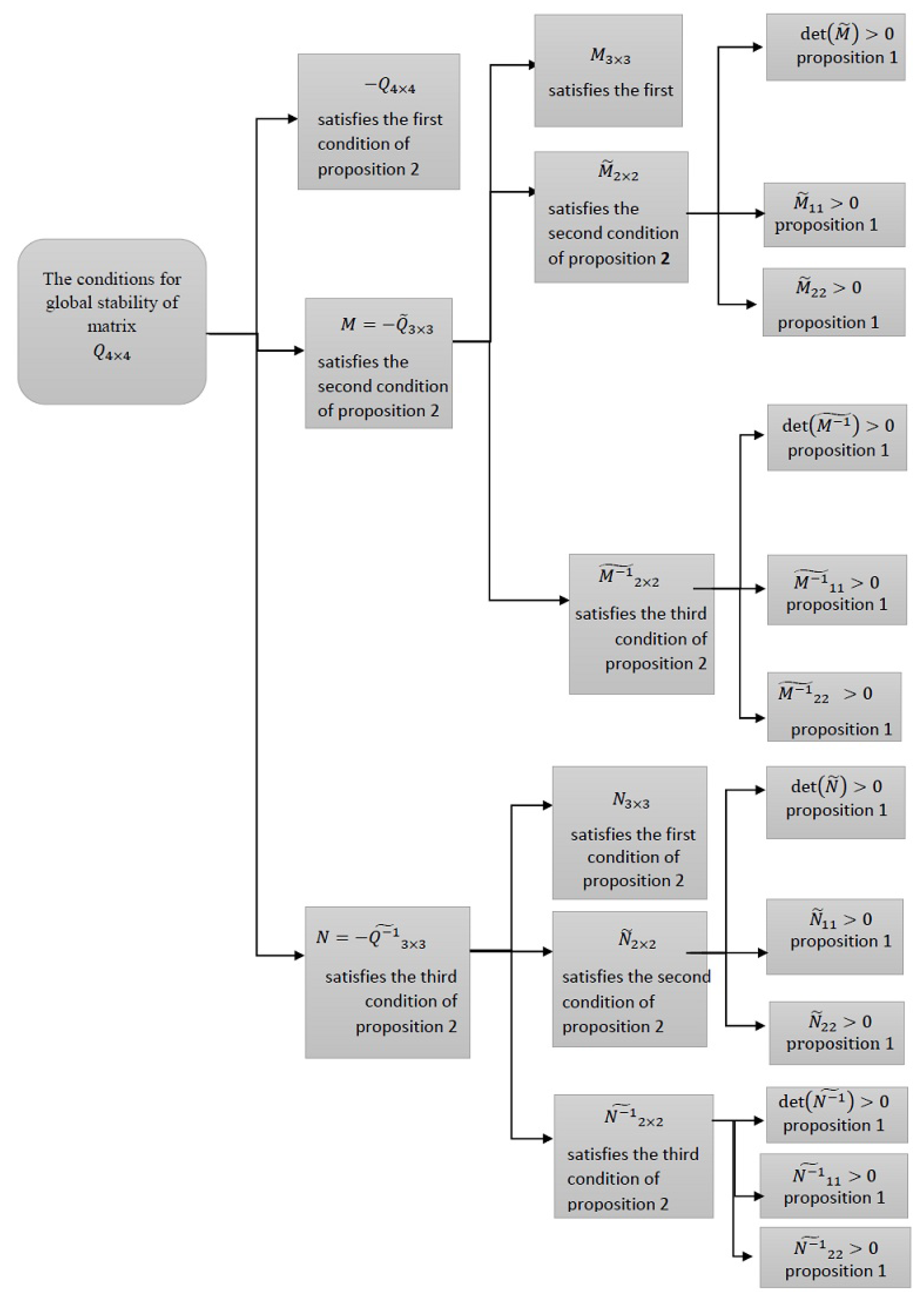
3.2. Global Stability of the Endemic Equilibrium

We study the system (1) in the biologically feasible domain

$$\begin{array}{c}\hfill \mathsf{\Gamma }=\left\{(S,E,I,R)\in {\mathbb{R}}_{+}^4:S\left(t\right)+E\left(t\right)+I\left(t\right)+R\left(t\right)=1\right\}.\end{array}$$

To begin the process, we define the Lyapunov function as follows:

$$\begin{array}{c}\hfill L=b_1{(S-S_e)}^2+b_2{(E-E_e)}^2+b_3{(I-I_e)}^2+b_4{(R-R_e)}^2,\end{array}$$

(7)

where $b_1, b_2, b_3$, and $b_4$ are positive constants. The time derivative of L is given by

$$\begin{array}{c}\frac{dL}{dt}=2b_1(S-S_e)\frac{dS}{dt}+2b_2(E-E_e)\frac{dE}{dt}+2b_3(I-I_e)\frac{dI}{dt}+2b_4(R-R_e)\frac{dR}{dt},\hfill \\ =2b_1(S-S_e)\left[\frac{-\beta SI}{1+aI}+\frac{\beta S_e{I}_e}{1+a{I}_e}-\nu (S-S_e)+\delta (R-R_e)\right]\hfill \\ +2b_2(E-E_e)\left[\frac{\beta SI}{1+aI}-\frac{\beta S_e{I}_e}{1+a{I}_e}-(ϵ+\nu )(E-E_e)\right]\hfill \\ +2b_3(I-I_e)\left[ϵ(E-E_e)-(\gamma +\nu )(I-I_e)\right]\hfill \\ +2b_4(R-R_e)\left[\gamma (I-I_e)-(\delta +\nu )(R-R_e)\right],\hfill \end{array}$$

and by doing some calculations, we have

$$\begin{array}{c}\frac{dL}{dt}=2b_1(S-S_e)\left[\frac{-\beta SI}{1+aI}+\frac{\beta S_e{I}_e}{1+a{I}_e}+\frac{\beta S_{e}I}{1+aI}-\frac{\beta S_{e}I}{1+aI}-\nu (S-S_e)+\delta (R-R_e)\right]\hfill \\ +2b_2(E-E_e)\left[\frac{\beta SI}{1+aI}-\frac{\beta S_e{I}_e}{1+a{I}_e}+\frac{\beta S_{e}I}{1+aI}-\frac{\beta S_{e}I}{1+aI}-(ϵ+\nu )(E-E_e)\right]\hfill \\ +2b_3(I-I_e)\left[ϵ(E-E_e)-(\gamma +\nu )(I-I_e)\right]\hfill \\ +2b_4(R-R_e)\left[\gamma (I-I_e)-(\delta +\nu )(R-R_e)\right].\hfill \end{array}$$

Therefore, we have

$$\begin{array}{cc}\hfill \frac{dL}{dt}& =-2b_1\frac{\beta I}{1+aI}{(S-S_e)}^2-2b_1\nu {(S-S_e)}^2+2b_1\delta (S-S_e)(R-R_e)\hfill \\ & -2b_1\frac{\beta S_e}{(1+aI)(1+a{I}_e)}(S-S_e)(I-I_e)+2b_2\frac{\beta I}{1+aI}(S-S_e)(E-E_e)\hfill \\ & -2b_2(ϵ+\nu ){(E-E_e)}^2+2b_2\frac{\beta S_e}{(1+aI)(1+a{I}_e)}(E-E_e)(I-I_e)\hfill \\ & +2b_3ϵ(I-I_e)(E-E_e)-2b_3(\gamma +\nu ){(I-I_e)}^2\hfill \\ & +2b_4\gamma (R-R_e)(I-I_e)-2b_4(\delta +\nu ){(R-R_e)}^2.\hfill \\ & =Y(BQ+Q^T{B}^T)Y^T,\hfill \end{array}$$

(8)

where $Y=[S-S_e,E-E_e,I-I_e,R-R_e],B=diag(b_1,b_2,b_3,b_4),$ and

$$\begin{array}{c}\hfill Q=\left[\begin{array}{cccc}-(\nu +\frac{\beta I}{1+aI})& 0& -\frac{\beta S_e}{(1+aI)(1+a{I}_e)}& \delta \\ \\ \frac{\beta I}{1+aI}& -(\nu +ϵ)& \frac{\beta S_e}{(1+aI)(1+a{I}_e)}& 0\\ \\ 0& ϵ& -(\gamma +\nu )& 0\\ \\ 0& 0& \gamma & -(\nu +\delta )\end{array}\right].\end{array}$$

(9)

Remark 1.

In the proposed method [23], Liao et al. met the following conditions to achieve the goal of stability of the matrix $C_{3\times 3}$.

(i) 

First, utilizing Proposition 1, they showed that ${(-C)}^{-1}$ is a Volterra-Lyapunov stable matrix.

(ii) 

The second step was to evaluate the Volterra-Lyapunov stability of matrix $-C.$ They must specify the matrices ${\tilde{B}}_{2\times 2}=diag(b_1,b_2)>0$ and $M_{2\times 2}>0$, such that

$$\begin{array}{c}\hfill \tilde{B}\widetilde{{(-C)}^{-1}}+{\left(\tilde{B}\widetilde{{(-C)}^{-1}}\right)}^T=\frac{1}{-det\left(C\right)}M>0.\end{array}$$

(iii) 

Finally, they considered

$$\begin{array}{c}\hfill \tilde{B}\widetilde{(-C)}+{\left(\tilde{B}\widetilde{(-C)}\right)}^T=N,\end{array}$$

and after some algebraic and matrix manipulations, it was concluded that $N_{2\times 2}>0.$

However, it is difficult to implement their method for high-dimensional systems.

The following Lemmas and theorems focus on the global stability of the endemic equilibrium $E_1$. To accomplish it, we must meet the conditions of Propositions 1 and 2. This process is illustrated in Figure 1.

Figure 1. Describing the presented method using Propositions 1 and 2.

Theorem 1.

Suppose that Equation (9) specifies the matrix $Q_{4\times 4}$; then, $Q_{4\times 4}$ is Volterra-Lyapunov stable.

Proof. 

Clearly, $-Q_{44}>0$. Let us delete the last row and last column of matrix $-Q$ and call it matrix $-\tilde{Q}.$ It follows that

$$\begin{array}{c}\hfill -\tilde{Q}=\left[\begin{array}{ccc}(\nu +\frac{\beta I}{1+aI})& 0& \frac{\beta S_e}{(1+aI)(1+a{I}_e)}\\ \\ -\frac{\beta I}{1+aI}& (\nu +ϵ)& -\frac{\beta S_e}{(1+aI)(1+a{I}_e)}\\ \\ 0& -ϵ& (\gamma +\nu )\end{array}\right]\end{array}$$

(10)

□

Now is the time to articulate Propositions 1 and 2. The following lemma does this for us.

Lemma 1.

The matrix $M=-\tilde{Q}$ is diagonally stable.

Proof. 

Here we discuss the diagonal stability of M, which is ensured by these conditions:

C1. Clearly, $M_{33}>0$.

C2. Let us define $\tilde{M}$ from (10), as follows:

$$\tilde{M}=\left[\begin{array}{cc}(\nu +\frac{\beta I}{1+aI})& 0\\ \\ -\frac{\beta I}{1+aI}& (\nu +ϵ)\end{array}\right].$$

Utilizing Proposition 1, we have ${\tilde{M}}_{11}>0, {\tilde{M}}_{22}>0$ and $\det (\tilde{M})>0.$ Accordingly, $\tilde{M}$ is diagonally stable.

C3. Finally, using Proposition 1, the diagonal stability of $\widetilde{M^{-1}}$ is determined. Let us delete the last row and last column of matrix $M^{-1}$ and define the matrix $\widetilde{M^{-1}}.$ We can derive

$$\begin{array}{c}\widetilde{M^{-1}}=\frac{1}{det\left(M\right)}\left[\begin{array}{cc}(\nu +ϵ)(\gamma +\nu )-\frac{\beta S_eϵ}{(1+aI)(1+a{I}_e)}& -\frac{\beta S_eϵ}{(1+aI)(1+a{I}_e)}\\ \\ \frac{\beta I}{1+aI}(\nu +\gamma )& (\nu +\frac{\beta I}{1+aI})(\nu +\gamma )\end{array}\right].\hfill \end{array}$$

Additionally, $det\left(M\right)$ can be obtained:

$$\begin{array}{c}\hfill det\left(M\right)=(\nu +ϵ)(\nu +\gamma )\left(\nu +\frac{\beta I}{1+aI}\right)-\frac{\nu \beta ϵS_e}{(1+aI)(1+a{I}_e)}.\end{array}$$

Then,

$$\begin{array}{cc}\hfill det\left(\widetilde{M^{-1}}\right)& =\frac{1}{{(det\left(M\right))}^2}\left((\nu +ϵ)(\nu +\gamma )-\frac{\beta S_eϵ}{(1+aI)(1+a{I}_e)}\right)\left(\nu +\frac{\beta I}{1+aI}\right)(\nu +\gamma )\hfill \\ & +\frac{\beta S_eϵ}{(1+aI)(1+a{I}_e)}(\nu +\gamma )\frac{\beta I}{1+aI}\hfill \\ & =\frac{1}{{(det\left(M\right))}^2}(\nu +ϵ){(\nu +\gamma )}^2(\nu +\frac{\beta I}{1+aI})>0.\hfill \end{array}$$

Evidently, ${\widetilde{M^{-1}}}_{22}>0$ and we have that $det\left(M\right)>0$, ${\widetilde{M^{-1}}}_{11}>0$ (see the Appendix A and Appendix B). Consequently, $\widetilde{M^{-1}}$ is diagonally stable. □

Lemma 2.

The matrix $\widetilde{Q^{-1}}$ is diagonally stable.

Proof. 

Based on Proposition 2, one can define $N=-\widetilde{Q^{-1}}$ as the following:

$$N=\frac{1}{det(-Q)}\left[\begin{array}{ccc}{N}_{11}& N_{12}& N_{13}\\ \\ N_{21}& N_{22}& N_{23}\\ \\ N_{31}& N_{32}& N_{33}\end{array}\right]$$

where,

$$\begin{array}{ccc}\hfill & \hfill & N_{11}=(\nu +ϵ)(\nu +\gamma )(\nu +\delta )-\frac{\beta S_eϵ(\nu +\delta )}{(1+aI)(1+a{I}_e)},\hfill \\ \hfill & \hfill & N_{12}=(\nu +\delta )\frac{\beta S_eϵ}{(1+aI)(1+a{I}_e)}+\delta ϵ\gamma ,\hfill \\ \hfill & \hfill & N_{13}=-(\nu +ϵ)(\nu +\delta )\frac{\beta S_e}{(1+aI)(1+a{I}_e)}+\delta \gamma (\nu +ϵ),\hfill \\ \hfill & \hfill & N_{21}=\frac{\beta I}{1+aI}(\gamma +\nu )(\nu +\delta ),\hfill \\ \hfill & \hfill & N_{22}=\left(\nu +\frac{\beta I}{1+aI}\right)(\nu +\gamma )(\nu +\delta ),\hfill \\ \hfill & \hfill & N_{23}=\left(\nu +\frac{\beta I}{1+aI}\right)\left(\frac{\beta S_e}{(1+aI)(1+a{I}_e)}(\nu +\delta )\right)+\frac{\beta S_e}{(1+aI)(1+a{I}_e)}\frac{\beta I}{1+aI}(\nu +\delta )-\frac{\beta I}{1+aI}\left(\delta \gamma \right),\hfill \\ \hfill & \hfill & N_{31}=\frac{\beta I}{1+aI}ϵ(\nu +\delta ),\hfill \\ \hfill & \hfill & N_{32}=\left(\nu +\frac{\beta I}{1+aI}\right)ϵ(\nu +\delta ),\hfill \\ \hfill & \hfill & N_{33}=\left(\nu +\frac{\beta I}{1+aI}\right)(\nu +ϵ)(\nu +\delta ).\hfill \end{array}$$

First, we show that $det(-Q)>0$:

$$\begin{array}{ll}det(-Q)& =\\ & \left(\nu +\frac{\beta I}{1+aI}\right)(\nu +\delta )(\nu +ϵ)(\nu +\gamma )-\nu ϵ(\nu +\delta )\frac{\beta S_e}{(1+aI)(1+a{I}_e)}-\frac{\beta I}{1+aI}\delta \gamma ϵ\\ & =\nu (\nu +\delta )(\nu +ϵ)(\nu +\gamma )+\left({\nu }^3+(\delta +\gamma +ϵ){\nu }^2+(\delta ϵ+\gamma \delta +\gamma ϵ)\nu \right)\frac{\beta I}{1+aI}\\ & -\nu (\nu +\delta )\frac{\beta S_eϵ}{(1+aI)(1+a{I}_e)}.\end{array}$$

(11)

From (3) and (4), we obtain

$$\begin{array}{c}\hfill (\nu +ϵ)(\nu +\gamma )=\frac{\beta S_eϵ}{1+a{I}_e},\end{array}$$

(12)

and then

$$\begin{array}{ll}det(-Q)\hfill & =\\ & \nu (\nu +\delta )\frac{\beta S_eϵ}{1+a{I}_e}\left(1-\frac{1}{1+aI}\right)+\left({\nu }^3+(\delta +\gamma +ϵ){\nu }^2+(\delta ϵ+\gamma \delta +\gamma ϵ)\nu \right)\frac{\beta I}{1+aI}\hfill \\ & =\nu (\nu +\delta )\frac{\beta S_eϵ}{1+a{I}_e}\left(\frac{aI}{1+aI}\right)+\left({\nu }^3+(\delta +\gamma +ϵ){\nu }^2+(\delta ϵ+\gamma \delta +\gamma ϵ)\nu \right)\frac{\beta I}{1+aI}>0.\hfill \end{array}$$

(13)

C1. It is clear that $N_{33}>0$.

C2. Now, we define $\tilde{N}$ from (10), in the form of

$$\tilde{N}=\frac{1}{det(-Q)}\left[\begin{array}{cc}{N}_{11}& N_{12}\\ N_{21}& N_{22}\end{array}\right].$$

It is straightforward to show that the conditions of Proposition 1 are satisfied, so that $det\left(\tilde{N}\right)>0.$ This ensures the diagonal stability of the matrix $\tilde{N}$.

C3. Utilizing Proposition 1, the diagonal stability of $\widetilde{N^{-1}}$ is determined. Let us delete the last row and last column of matrix $N^{-1}$ and define the matrix $\widetilde{N^{-1}}$:

$$\widetilde{N^{-1}}=\left[\begin{array}{cc}\nu +\frac{\beta I}{1+aI}& 0\\ \\ \frac{-\beta I}{1+aI}& \nu +ϵ\end{array}\right].$$

Obviously, ${\widetilde{N^{-1}}}_{11}>0$ and ${\widetilde{N^{-1}}}_{22}>0$ and $det\left(\widetilde{N^{-1}}\right)>0$. Therefore, one can conclude that $\widetilde{N^{-1}}$ is diagonally stable.

Finally, because matrix N satisfies the conditions of Proposition 2, $N=-\widetilde{Q^{-1}}$ is therefore diagonally stable. □

Lemmas 1 and 2 show that the three conditions of Proposition 2 are met, and as a result, the matrix Q is Volterra-Lyapunov stable. This completes the proof.

Theorem 2.

When $R_0>1,$ the endemic equilibrium $E_1=(S_e,E_e,I_e,R_e)$ of model (1) is globally asymptotically stable in Γ.

Proof. 

In Theorem 1, the existence of a positive diagonal matrix B is guaranteed so that $B(-Q)+{(-Q)}^T{B}^T>0.$ Thus, we have $BQ+Q^T{B}^T<0.$ Therefore, $\frac{dL}{dt}<0$, and this ensures the global stability of the endemic equilibrium point. □

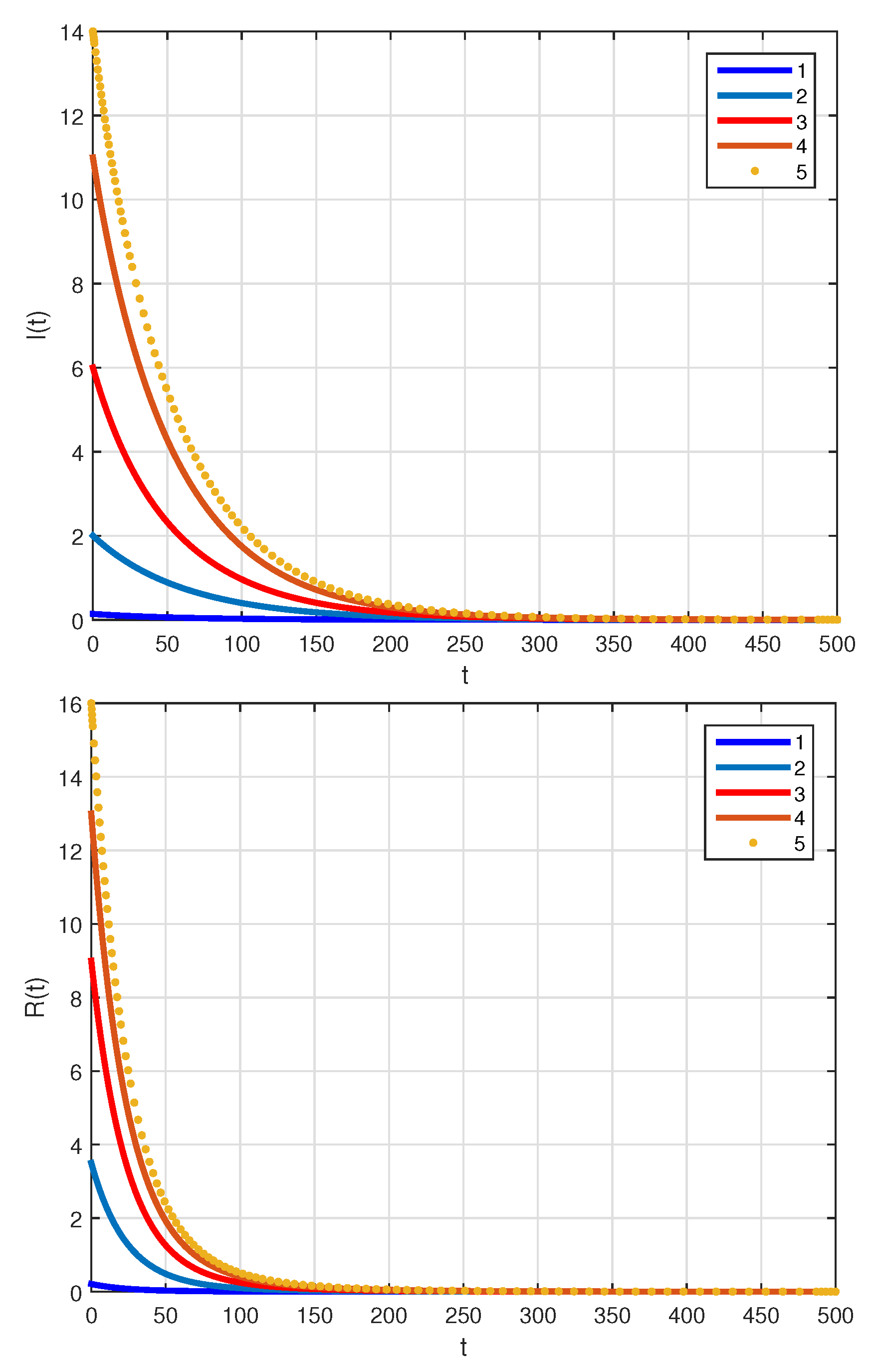
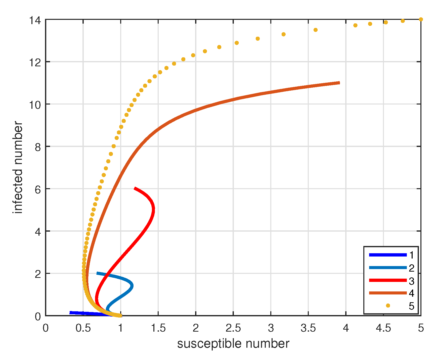
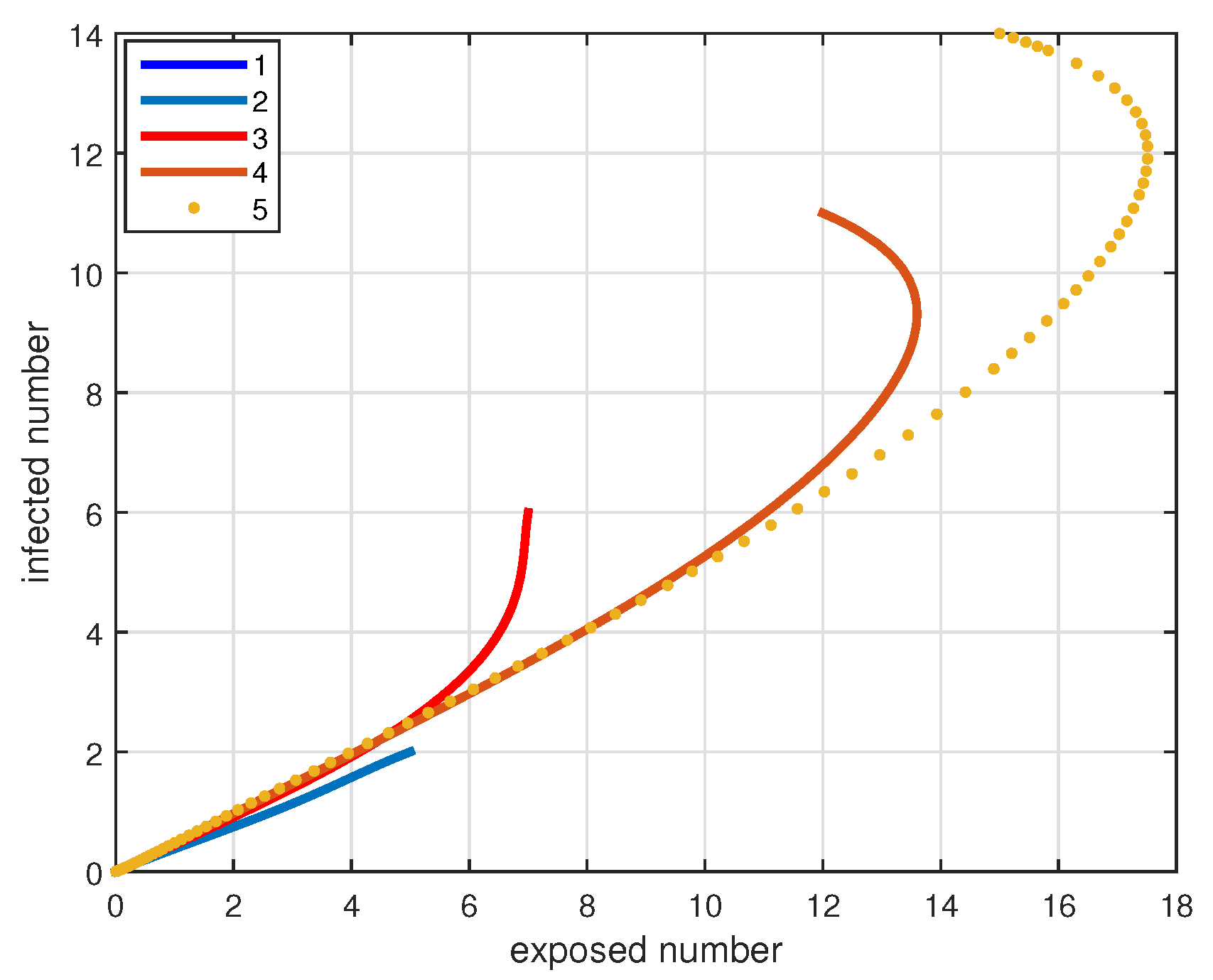
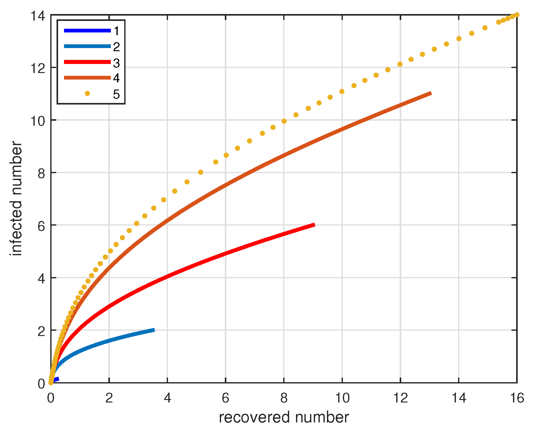
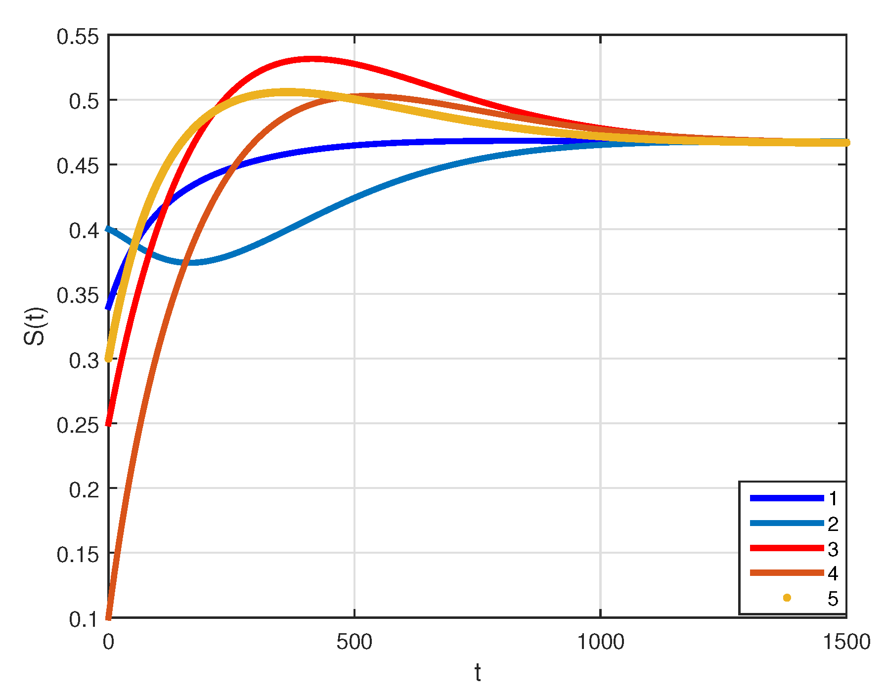
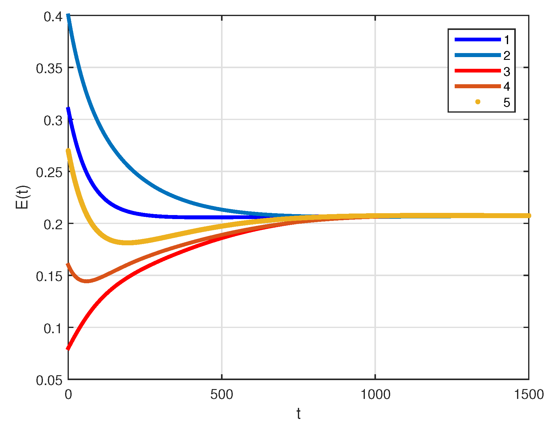
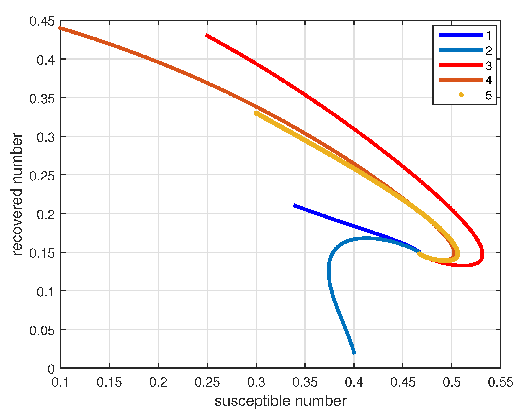
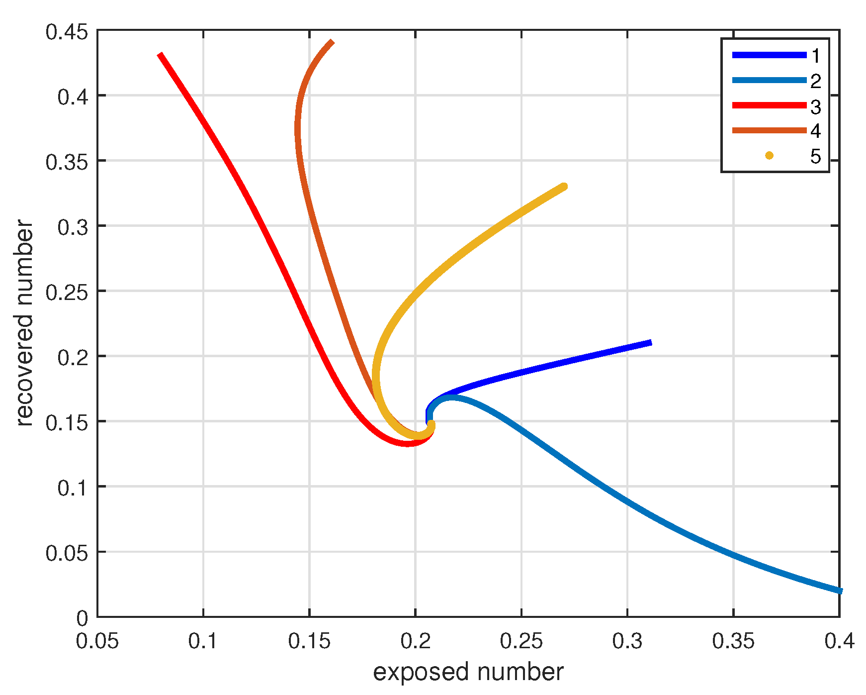
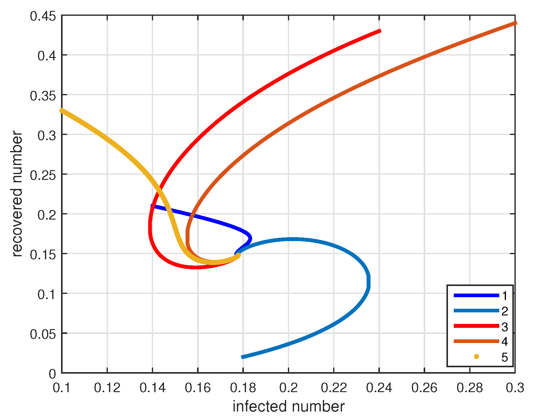
4. Numerical Simulations and Discussions

In this section, we numerically assess Theorem 2 by means of two examples.

Example 1.

Consider system (1) with the parameters $\beta =0.02,\nu =0.02,\delta =0.024,ϵ=0.003,\gamma =0.004$, and $a=0.004$ [20].

The basic reproduction number is such that $R_0=0.1087<1$ and the system (1) has only the disease-free equilibrium of $E_0=(1,0,0,0)$. We take the following five initial conditions:

• $S\left(0\right)=0.34,E\left(0\right)=0.31,I\left(0\right)=0.14$ and $R\left(0\right)=0.21,$
• $S\left(0\right)=0.7,E\left(0\right)=5,I\left(0\right)=2$ and $R\left(0\right)=3.5,$
• $S\left(0\right)=1.2,E\left(0\right)=7,I\left(0\right)=6$ and $R\left(0\right)=9,$
• $S\left(0\right)=3.9,E\left(0\right)=12,I\left(0\right)=11$ and $R\left(0\right)=13,$
• $S\left(0\right)=5,E\left(0\right)=15,I\left(0\right)=14$ and $R\left(0\right)=16.$

The numerical simulation of system (1) with five different initial conditions is illustrated in Figure 2 and Figure 3, where all orbits converge to $E_0$.

Figure 2. The evolution dynamics of susceptible and exposed population vs. time, $R_0=0.1087<1.$

Figure 3. The evolution dynamics of infected and removed population vs. time, $R_0=0.1087<1.$

In Figure 4, we observe five solution curves by the phase portrait of I vs. S, corresponding to five initial conditions. In Figure 5, we plot the phase portrait of I vs. E and see that five solutions converge to the $E_0$ with five different initial conditions. In Figure 6, we have five solutions and the phase portrait of I vs. R. Therefore, it can be seen from these figures that all solutions approach the disease-free equilibrium point under the mentioned initial conditions.

Figure 4. The phase portraits of I vs. S for system (1). The five trajectories correspond to different initial conditions and $R_0=0.1087<1.$

Figure 5. The phase portraits of I vs. E for system (1). The five trajectories correspond to different initial conditions and $R_0=0.1087<1.$

Figure 6. The phase portraits of I vs. R for system (1). The five trajectories correspond to different initial conditions and $R_0=0.1087<1.$

Example 2.

Consider the system (1) with the parameters β = 0.02, ν = 0.002, δ = 0.004, ϵ = 0.006, γ = 0.005 and a = 0.004 [20].

The basic reproduction number is such that $R_0=2.1429>1,$ and system (1) has the endemic equilibrium $E_1=(S_e,E_e,I_e,R_e)$. The simulation of system (1) with the same conditions is depicted in Figure 7 and Figure 8.

Figure 7. The evolution dynamics of susceptible and exposed population against time, using initial state values and $R_0=2.1429>1.$

Figure 8. The evolution dynamics of infected and removed population against time, using initial state values and $R_0=2.1429>1.$

• $S\left(0\right)=0.34,E\left(0\right)=0.31,I\left(0\right)=0.14$ and $R\left(0\right)=0.21,$
• $S\left(0\right)=0.4,E\left(0\right)=0.4,I\left(0\right)=0.18$ and $R\left(0\right)=0.02,$
• $S\left(0\right)=0.25,E\left(0\right)=0.08,I\left(0\right)=0.24$ and $R\left(0\right)=0.43,$
• $S\left(0\right)=0.1,E\left(0\right)=0.16,I\left(0\right)=0.3$ and $R\left(0\right)=0.44,$
• $S\left(0\right)=0.3,E\left(0\right)=0.27,I\left(0\right)=0.1$ and $R\left(0\right)=0.33.$

We verify that orbits converge to the $E_1\approx (0.4656,0.2078,0.1781,0.1485)$. The corresponding phase portraits of R vs. S with the above different initial conditions are depicted in Figure 9, which demonstrates the globally asymptotic stability of endemic equilibrium $E_1$. Further, the state portraits of R vs. E, with five different initial conditions, is depicted in Figure 10, that displays the global asymptotic stability of $E_1$. In Figure 11, we plot the phase portrait of R vs. I corresponding to these initial conditions. The figures confirm that the endemic equilibrium $E_1$ is globally asymptotically stable, and all solutions converge to $E_1$ under the mentioned initial conditions.

Figure 9. The phase portraits of R vs. S for system (1). The five trajectories correspond to different initial conditions and $R_0=2.1429>1.$

Figure 10. The phase portraits of R vs. E for system (1). The five trajectories correspond to different initial conditions and $R_0=2.1429>1.$

Figure 11. The phase portraits of R vs. I for system (1). The trajectories correspond to different initial conditions and $R_0=2.1429>1.$

5. Conclusions

This paper considered the epidemic SEIRS model with the nonlinear incidence rate $\frac{\beta SI}{1+aI}$. The conditions for the global stability of the endemic equilibrium were established using the theory of Volterra-Lyapunov stable matrices. The method we implemented minimizes the problems of the method presented in Remark 1. This strategy simplifies the calculations and the proofs. The numerical simulations confirm the theoretical results.

References

- Kumar, A. Mathematical analysis of a delayed epidemic model with nonlinear incidence and treatment rates. J. Eng. Math. 2019, 115, 1–20. [Google Scholar] [CrossRef]
- Baba, I.A.; Hincal, E. Global stability analysis of two-strain epidemic model with bilinear and non-monotone incidence rates. Eur. Phys. J. Plus 2017, 132, 208. [Google Scholar] [CrossRef]
- Wang, Y.; Cao, J. Global stability of general cholera models with nonlinear incidence and removal rates. J. Frankl. Inst. 2015, 352, 2464–2485. [Google Scholar] [CrossRef]
- Geng, Y.; Xu, J. Stability preserving NSFD scheme for a multi-group SVIR epidemic model. Math. Methods Appl. Sci. 2017, 40, 4917–4927. [Google Scholar] [CrossRef]
- Huang, G.; Nie, C.; Dong, Y. Global stability for an SEI model of infectious diseases with immigration and age structure in susceptibility. Int. J. Biomath. 2019, 12, 1950042. [Google Scholar] [CrossRef]
- Li, Y.; Zhang, L.; Guo, G. The asymptotic stability for an SIQS epidemic model with diffusion. Int. J. Biomath. 2016, 9, 1650015. [Google Scholar] [CrossRef] [Green Version]
- Eskandari, Z.; Alidousti, J. Stability and codimension 2 bifurcations of a discrete time SIR model. J. Frankl. Inst. 2020, 357, 10937–10959. [Google Scholar] [CrossRef]
- Agha, A.A.; Alshehaiween, S.; Elaiw, A.; Alshaikh, M. A global analysis of delayed SARS-CoV-2/cancer model with immune response. Mathematics 2021, 9, 1283. [Google Scholar] [CrossRef]
- Wang, J.; Liao, S. A generalized cholera model and epidemic-endemic analysis. J. Biol. Dyn. 2012, 6, 568–589. [Google Scholar] [CrossRef] [PubMed]
- Hu, Z.; Ma, W.; Ruan, S. Analysis of SIR epidemic models with nonlinear incidence rate and treatment. Math. Biosci. 2012, 238, 12–20. [Google Scholar] [CrossRef] [PubMed]
- Hethcote, H.W.; van den Dreissche, P. Some epidemiological models with nonlinear incidence rate. J. Math. Biol. 1991, 29, 271–287. [Google Scholar] [CrossRef] [Green Version]
- Li, M.Y.; Muldowney, J.S.; van den Dreissche, P. Global stability of the SEIRS model in epidemiology. Can. Appl. Math. Quart. 1999, 7, 409–425. [Google Scholar] [CrossRef]
- Keeling, M.J.; Rohani, P.; Grenfell, B.T. Seasonally forced disease dynamics explored as switching between attractors. Phys. D Nonlinear Phenom. 2001, 148, 317–335. [Google Scholar] [CrossRef]
- Xiao, D.; Ruan, S. Global analysis of an epidemic model with nonmonotone incidence rate. Math. Biosci. 2007, 208, 419–429. [Google Scholar] [CrossRef]
- Liu, W.M.; Levin, S.A.; Iwasa, Y. Influence of nonlinear incidence rates upon the behavior of SIRS epidemiological models. J. Math. Biol. 1986, 23, 187–204. [Google Scholar] [CrossRef] [PubMed]
- Rohith, G.; Devika, K.B. Dynamics and control of COVID-19 pandemic with nonlinear incidence rates. Nonlinear Dyn. 2020, 101, 2013–2026. [Google Scholar] [CrossRef] [PubMed]
- Bentaleb, D.; Amine, S. Lyapunov function and global stability for a two-strain SEIR model with bilinear and nonmonotone incidence. Int. J. Biomath. 2019, 12, 1950021. [Google Scholar] [CrossRef]
- Chen, Y.; Li, J.; Zou, S. Global dynamics of an epidemic model with relapse and nonlinear incidence. Math. Methods Appl. Sci. 2019, 42, 1283–1291. [Google Scholar] [CrossRef]
- Zhang, H.; Xia, J.; Georgescu, P. Multigroup deterministic and stochastic SEIRI epidemic models with nonlinear incidence rates and distributed delays: A stability analysis. Math. Methods Appl. Sci. 2017, 40, 6254–6275. [Google Scholar] [CrossRef]
- Zheng, L.; Yang, X.; Zhang, L. On global stability analysis for SEIRS models in epidemiology with nonlinear incidence rate function. Int. J. Biomath. 2017, 10, 1750019. [Google Scholar] [CrossRef]
- Upadhyay, R.K.; Pal, A.K.; Kumari, S.; Roy, P. Dynamics of an SEIR epidemic model with nonlinear incidence and treatment rates. Nonlinear Dyn. 2019, 96, 2351–2368. [Google Scholar] [CrossRef]
- Lv, W.; Ke, Q.; Li, K. Dynamic stability of an SIVS epidemic model with imperfect vaccination on scale-free networks and its control strategy. J. Frankl. Inst. 2020, 357, 7092–7121. [Google Scholar] [CrossRef]
- Liao, S.; Wang, J. Global stability analysis of epidemiological models based on Volterra-Lyapunov stable matrices. Chaos Solitons Fractals 2012, 45, 966–977. [Google Scholar] [CrossRef]
- Parsaei, M.R.; Javidan, R.; Shayegh Kargar, N.; Saberi Nik, H. On the global stability of an epidemic model of computer viruses. Theory Biosci. 2017, 136, 169–178. [Google Scholar] [CrossRef]
- Masoumnezhad, M.; Rajabi, M.; Chapnevis, A.; Dorofeev, A.; Shateyi, S.; Karga, N.S.; Saberi Nik, H. An approach for the global stability of mathematical model of an infectious disease. Symmetry 2020, 12, 1778. [Google Scholar] [CrossRef]
- Zahedi, M.S.; Kargar, N.S. The Volterra-Lyapunov matrix theory for global stability analysis of a model of the HIV/AIDS. Int. J. Biomath. 2017, 10, 1750002. [Google Scholar] [CrossRef]
- Tian, J.P.; Wang, J. Global stability for cholera epidemic models. Math. Biosci. 2011, 232, 31–41. [Google Scholar] [CrossRef] [PubMed]
- Driessche, V.D.; Watmough, J. Reproduction numbers and sub-threshold endemic equilibria for compartmental models of disease transmission. Math. Biosci. 2002, 180, 29–48. [Google Scholar] [CrossRef]
- Cross, G.W. Three types of matrix stability. Linear Algebra Appl. 1978, 20, 253–263. [Google Scholar] [CrossRef] [Green Version]
- Rinaldi, F. Global stability results for epidemic models with latent period. IMA J. Math. Appl. Med. Biol. 1990, 7, 69–75. [Google Scholar] [CrossRef]
- Redheffer, R. Volterra multipliers I. SIAM J. Algebraic Discret. Methods 1985, 6, 592–611. [Google Scholar] [CrossRef]
- Redheffer, R. Volterra multipliers II. SIAM J. Algebraic Discret. Methods 1985, 6, 612–623. [Google Scholar] [CrossRef]
Publisher’s Note: MDPI stays neutral with regard to jurisdictional claims in published maps and institutional affiliations. |
© 2021 by the authors. Licensee MDPI, Basel, Switzerland. This article is an open access article distributed under the terms and conditions of the Creative Commons Attribution (CC BY) license (https://creativecommons.org/licenses/by/4.0/).