
A Fusion Framework for Forecasting Financial Market Direction Using Enhanced Ensemble Models and Technical Indicators

 ,
,  ,
,
Abstract
:1. Introduction
1.1. The Inspiration Is as per the Following
1.2. Our Research Contributions in a Nutshell
- We propose a novel framework where six ensemble models are hybridised, minimising the model risk and increasing accuracy.
- A new set of input features were designed, providing a real test for future researchers to think of that combination.
- In this approach, we adopted two-phase overfitting protection. The first is LDA, and the second is the K-fold cross-validation. These techniques were merged into a single framework, making our model a unique one.
- Our model selection process is somewhat different and uncommon. Instead of selecting the model which provides the highest accuracy, we selected the model whose training and testing accuracy difference is minimal, which is very much uncommon and innovative, and this selection process produces a model neither overfitted nor underfitted.
- Specifically, a long time period of data was collected for our experimental setup, which explores the performance level of volatility–stress periods and smooth trending periods and it also examines the persistence of financial crisis and clustering.
2. Related Work
2.1. Statistical Technique
2.2. Machine Learning Technique
3. Materials and Methods
3.1. Ensemble Learning
3.1.1. Gradient Boosting
- Initially, develop an error function, and that function is optimised at the time of model building.
- Iteratively develop weak models for forecasting.
- Finally, all the weak models are merged a create a robust model with minimising error function.
3.1.2. AdaBoost
3.1.3. Extreme Gradient Boosting (XGBoost)
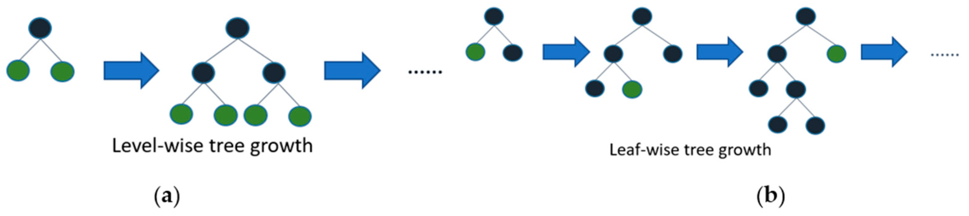
3.1.4. The LightGBM
3.1.5. CatBoost
3.1.6. Histogram Gradient Boosting
3.2. Dimensionality Reduction Technique
3.3. Evaluation Matrices
- represents the total number of true positive values;
- represents the total number of true negative values;
- represents the total number of false positive values;
- represents the total number of false negative values.
3.4. Tools and Technologies Used
3.5. Dataset
Data Pre-Processing
- (a)
- Generally, the index extracted from the web portal has some existing features that are open, close, low, high, etc. Now, looking at the dataset, we had to handle the null and missing values.
- (b)
- In the second step, we extracted 23 technical indicators using the preexisting dataset described in the previous point. Apart from the technical indicators, we extracted two more features, i.e., the difference between the open and close price, which reflects the increase and decrease of stock value on that day. Another one is to find out the volatility, i.e., the difference between high and low stock prices.
- (c)
- Label generation: In label generation, we constructed a response predicted variable, the binary feedback variable, i.e., Zt ∈ {0, 1}, for individual trading days of our stock. The feedback variable that will be forecast on the T’th day is calculated asZt is the forecast label labelled as ‘TREND’ that is used as our predicted variable, Open is the opening price of the index on the day, and Closet is the closing price of the index on the day. Here, we assume that when the Zt value returns ‘1’, the stock price will increase, and when the Zt value returns ‘0’, we consider the stock price to have decreased.If Opent < Closet
Then
Zt = 1
Else
Zt = 0
End If - (d)
- Although we are dealing with technical indicators representing a stock’s hidden behaviour, we must find a perfect combination of input features with no multi-collinearity issues. The problems with multi-collinearity from a mathematical viewpoint are that the coefficient gauges themselves will, in general, be untrustworthy and that variable is not measurably critical; because of these disadvantages, we ought to consistently check for multi-collinearity in our dataset. For checking multi-collinearity, we have to create a corelation matrix with the help of the correlation function corr(·) (which is used to find the pairwise correlation of all columns in the dataframe) function. This function creates a matrix with a correlation value with the combination of each variable. Therefore, when we diagonally check the matrix, we will obtain correlation values. By looking at the matrix, we have to remove the features whose values are more than 50. Thus, quickly looking at the matrix, we can easily identify the highly correlated values, which should be released. During this feature selection process, we used 23 technical indicators along with seven standard features. After successful correlation testing, we found only seven input features perfectly combined and ready to train our model.
- F_ma (fast-moving average for a short period);
- S_ma (slow-moving average for a long period).
- (e)
- After obtaining the useful features, we divided our database into two parts: 75% of the data reserve for training and 25% of the data to test our predictive model.
- (f)
- Finally, in the data processing step, we implemented the scaling technique to normalise our features, which are to be inputted into our model. The statistical description of our three datasets are provided below in Table 2, Table 3, Table 4, Table 5 and Table 6, in which we exploit each of the features of max, min, mean, and standard deviation values of all three datasets.
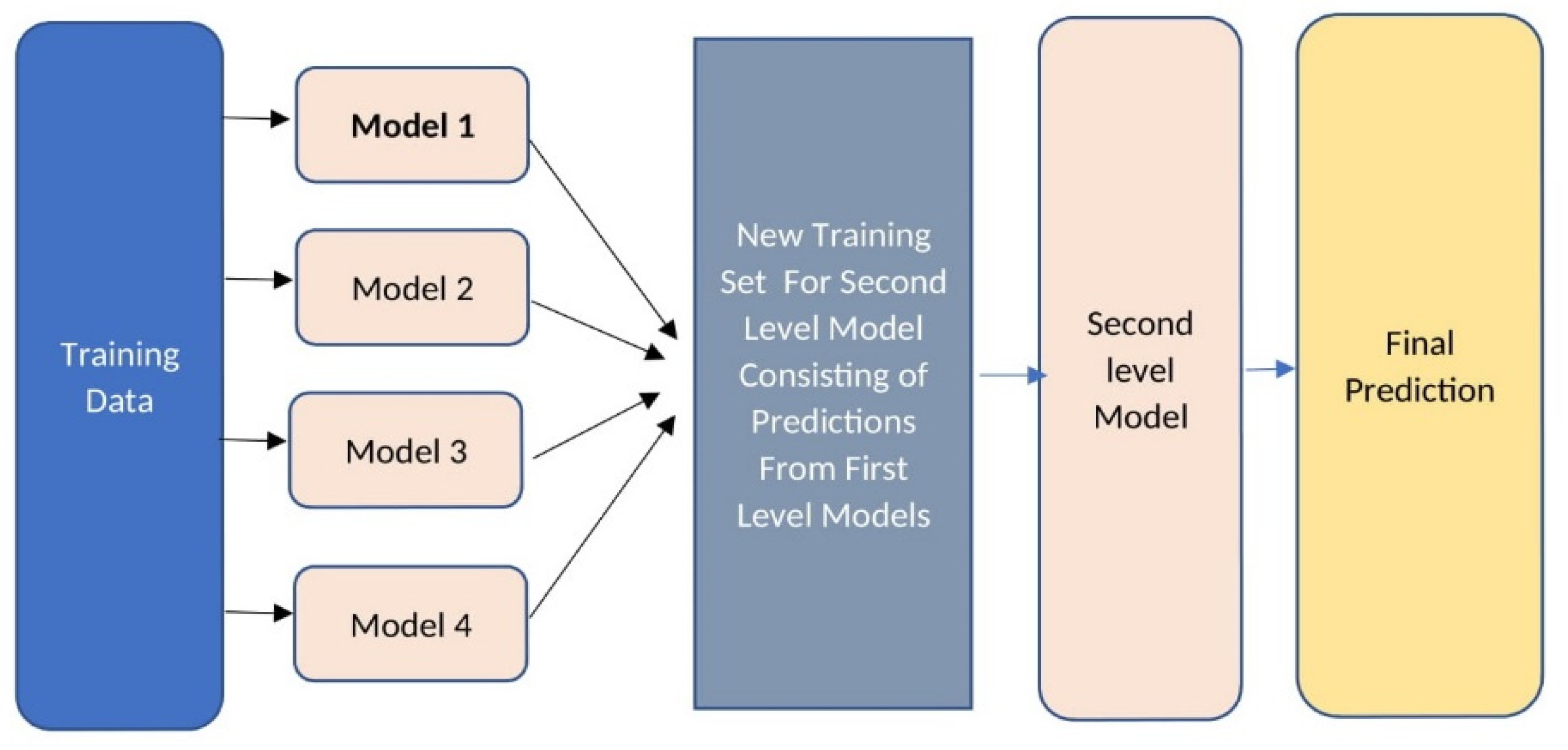
4. Proposed Framework
| Algorithm 1. Pseudocode for the proposed framework. |
| 1: Input: Training data |
| 2: Output: A boosted stacking meta classifier model denoted as M |
| 3: Step 1: Implementation of dimensional reduction technique to prepare a training set for base-level classifiers. |
| 4: Step 2: Initialise E to 6 (number of base-level classifiers) |
| 5: For i < −1 to E do |
| 6: Read the baselevel classifier mi |
| 7: Prepare a training set for first level classifiers |
| 8: For t < −1 to d do |
| 9: Train the model |
| 10: mi (t) |
| 11: end for |
| 12: fmi < −mi |
| 13: end for |
| 14: Step 3: Read the level-2 meta classifier |
| 15: Train the meta-classifier with cross-validation technique |
| 16: For j < −1 to E do |
| 17: For i < −1 to E do |
| 18: Ds = Ds + fmi |
| 19: End for |
| 20: Create a meta-classifier |
| 21: M (Ds) |
| 22: End for |
| 23: Step 4: Return (M) |
5. Results and Discussion
5.1. Performance of Base-Level Classifiers
5.2. Performances of Fusion-Based Meta-Classifiers
5.2.1. Performances of DJIA Index
5.2.2. Performance of HSI
5.2.3. Performance of S&P-500 Index
5.2.4. Performance of DAX Index
5.2.5. Performance of NIKKEI 225 Index
5.3. Evalution Matrices of Meta-LightGBM
5.4. Forecast Accuracy Comparison with Past Work
5.5. Practical Implications
6. Conclusions and Future Scope
Limitations and Future Work
Author Contributions
Funding
Institutional Review Board Statement
Informed Consent Statement
Data Availability Statement
Acknowledgments
Conflicts of Interest
Abbreviations
| CLAHE | Contrast-limited adaptive histogram equalisation |
| PSNR | Peak signal-to-noise ratio |
| PCA | Principal component analysis |
| ICA | Independent component analysis |
| FF | Firefly |
| HO | Hybrid optimisation |
| MAE | Mean absolute error |
References
- Adam, K.; Marcet, A.; Nicolini, J.P. Stock Market Volatility and Learning. J. Financ. 2016, 71, 33–82. [Google Scholar] [CrossRef] [Green Version]
- Kunze, F.; Spiwoks, M.; Bizer, K. The usefulness of oil price forecasts—Evidence from survey predictions. Manag. Decis. Econ. 2018, 39, 427–446. [Google Scholar] [CrossRef]
- Agustini, W.F.; Affianti, I.R.; Putri, E. Stock price prediction using geometric Brownian motion. J. Phys. Conf. Ser. 2018, 974, 012047. [Google Scholar] [CrossRef] [Green Version]
- Dinh, T.A.; Kwon, Y.K. An empirical study on importance of modeling parameters and trading volume-based features in daily stock trading using neural networks. IEEE Inform. 2018, 5, 36. [Google Scholar] [CrossRef] [Green Version]
- Mehdizadeh, S.; Sales, A.K. A comparative study of autoregressive, autoregressive moving average, gene expression programming and Bayesian networks for estimating monthly streamflow. Water Resour. Manag. 2018, 32, 3001–3022. [Google Scholar] [CrossRef]
- Zhang, Y.; Song, W.; Karimi, M.; Chi, C.H. Kudreyko, AFractional autoregressive integrated moving average and finite-element modal: The forecast of tire vibration trend. IEEE Access 2018, 6, 40137–40142. [Google Scholar] [CrossRef]
- Li, Q.; Cao, G.; Wei, X. Relationship research between meteorological disasters and stock markets based on a multifractal detrending moving average algorithm. Int. J. Mod. Phys. 2018, 32, 1750267. [Google Scholar] [CrossRef]
- Petukhova, T.; Ojkic, D.; McEwen, B.; Deardon, R.; Poljak, Z. Assessment of autoregressive integrated moving average (ARIMA), generalized linear autoregressive moving average (GLARMA), and random forest (RF) time series regression models for predicting influenza a virus frequency in swine in Ontario, Canada. PLoS ONE 2018, 13, e0198313. [Google Scholar] [CrossRef]
- Wang, D.; Liang, Z. Afuzzy set-valued autoregressive moving average model and its applications. Symmetry 2018, 10, 324. [Google Scholar] [CrossRef] [Green Version]
- Rui, R.; Wu, D.D.; Liu, T. Forecasting stock market movement direction using sentiment analysis and support vector machine. IEEE Syst. J. 2018, 13, 60–770. [Google Scholar]
- Nabipour, M.; Nayyeri, P.; Jabani, H.; Mosavi, A.; Salwana, E.S.S. Deep Learning for Stock Market Prediction. Entropy 2020, 22, 840. [Google Scholar] [CrossRef]
- Jothimani, D.; Surendra, S.Y. Stock trading decisions using ensemble based forecasting models: A study of the Indian stock market. J. Bank. Financ. Technol. 2019, 3, 113–129. [Google Scholar] [CrossRef]
- Zhong, X.; Enke, D. Predicting the daily return direction of the stock market using hybrid machine learning algorithms. Financ. Innov. 2019, 5, 24. [Google Scholar] [CrossRef]
- Yu, L.; Hu, L.; Tang, L. Stock Selection with a Novel Sigmoid-Based Mixed Discrete-Continuous Differential Evolution Algorithm. IEEE Trans. Knowl. Data Eng. 2016, 28, 1891–1904. [Google Scholar] [CrossRef]
- Shen, J.; Shafiq, M.O. Short-term stock market price trend prediction using a comprehensive deep learning system. J. Big Data 2020, 7, 66. [Google Scholar] [CrossRef] [PubMed]
- Qiu, M.; Song, Y.; Akagi, F. The case of the Japanese stock market. Chaos Solitons Fractals 2016, 85, 1–7. [Google Scholar] [CrossRef]
- Salim, L. A Technical Analysis Information Fusion Approach for Stock Price Analysis and Modeling. World Sci. Res. 2018, 17, 1850007. [Google Scholar]
- Weng, B.; Martinez, W.; Tsai, Y.-T.; Li, C.; Lu, L.; Barth, J.R.; Megahed, F.M. Macroeconomic indicators alone can predict the monthly closing price of major U.S. indices: Insights from artificial intelligence, time-series analysis and hybrid models. Appl. Soft Comput. 2018, 71, 685–697. [Google Scholar] [CrossRef]
- Fama, E.F. Random walks in stock market prices. Financ. Anal. J. 1965, 21, 55–59. [Google Scholar] [CrossRef] [Green Version]
- Malkiel, B.G.; Fama, E.F. Efficient capital markets: A review of theory and 810 empirical work. J. Financ. 1970, 25, 383–417. [Google Scholar] [CrossRef]
- Kahneman, D.; Tversky, A. Prospect Theory: An Analysis of Decision under Risk. Econometrica 1979, 47, 263–291. [Google Scholar] [CrossRef] [Green Version]
- Glogowski, J. Keeping Up with the Quants: Your Guide to Understanding and Using Analytics by Thomas, H. Davenport and Jinho Kim. J. Bus. Financ. Librariansh. 2014, 19, 86–89. [Google Scholar] [CrossRef]
- Rosenberg, B.; Reid, K.; Lanstein, R. Persuasive Evidence of Market Inefficiency. J. Portf. Manag. 1985, 13, 9–17. [Google Scholar] [CrossRef]
- Sanjoy, B. Investment Performance of Common Stocks in Relation to Their Price-Earnings Ratios: A test of the Efficient Markets Hypothesis. J. Financ. 1977, 32, 663–682. [Google Scholar]
- Nti, I.K.; Adekoya, A.F.; Weyori, B.A. A systematic review of fundamental and technical analysis of stock market predictions. Artif. Intell. Rev. 2020, 53, 3007–3057. [Google Scholar] [CrossRef]
- Shiller, R.J. From efficient markets theory to behavioral finance. J. Econ. Perspect. 2003, 17, 83–104. [Google Scholar] [CrossRef] [Green Version]
- Thaler, R.H. The end of behavioral finance. Financ. Anal. J. 1999, 55, 12–17. [Google Scholar] [CrossRef] [Green Version]
- Hsu, P.H.; Kuan, C.M. Reexamining the profitability of technical analysis with data snooping checks. J. Financ. Econom. 2005, 3, 606–628. [Google Scholar] [CrossRef] [Green Version]
- Nguyen, T.H.; Shirai, K.; Velcin, J. Sentiment analysis on social media for stock movement prediction. Expert Syst. Appl. 2015, 42, 9603–9611. [Google Scholar] [CrossRef]
- Dreman, D.N.; Berry, M.A. Overreaction, Underreaction, and the Low-P/E Effect. Financ. Anal. J. 1995, 51, 21–30. [Google Scholar] [CrossRef]
- Anbalagan, T.; Maheswari, S.U. Classifcation and prediction of stock market index based on fuzzy metagraph. Procedia Comput. Sci. 2014, 47, 214–221. [Google Scholar] [CrossRef] [Green Version]
- Ghaznavi, A.; Aliyari, M.; Mohammadi, M.R. Predicting stock price changes of tehran artmis company using radial basis function neural networks. Int. Res. J. Appl. Basic Sci. 2014, 10, 972–978. [Google Scholar]
- Agarwal, P.; Bajpai, S.; Pathak, A.; Angira, R. Stock market price trend forecasting using machine learning. Int. J. Res. Appl Sci. Eng. Technol. 2017, 5, 1673–1676. [Google Scholar]
- Schmeling, M. Investor sentiment and stock returns: Some international evidence. J. Empir. Financ. 2009, 16, 394–408. [Google Scholar] [CrossRef] [Green Version]
- Hu, Y.; Liu, K.; Zhang, X.; Su, L.; Ngai EW, T.; Liu, M. Application of evolutionary computation for rule discovery in stock algorithmic trading: A literature review. Appl. Soft Comput. 2015, 36, 534–551. [Google Scholar] [CrossRef]
- Khan, H.Z.; Alin, S.T.; Hussain, A. Price prediction of share market using artifcial neural network “ANN”. Int. J. Comput. Appl. 2011, 22, 42–47. [Google Scholar]
- Ballings, M.; Dirk, V.P.; Nathalie, H.; Ruben, G. Evaluating multiple classifiers for stock price direction prediction. Expert Syst. Appl. 2015, 42, 7046–7056. [Google Scholar] [CrossRef]
- Schapire, R.E. Explaining AdaBoost. In Empirical Inference; Schölkopf, B., Luo, Z., Vovk, V., Eds.; Springer: Berlin/Heidelberg, Germany, 2019. [Google Scholar]
- Su, C.H.; Cheng, C.H. A hybrid fuzzy time series model based on ANFIS and integrated nonlinear feature selection method for forecasting stock. Neurocomputing 2016, 205, 264–273. [Google Scholar] [CrossRef]
- Padhi, D.K.; Padhy, N. Prognosticate of the financial market utilizing ensemble-based conglomerate model with technical indicators. Evol. Intel. 2021, 14, 1035–1051. [Google Scholar] [CrossRef]
- Marwala, T.; Hurwitz, E. Artificial Intelligence and Economic Theory: Skynet in the Market; Springer: London, UK, 2017. [Google Scholar]
- Malkiel, B.G. The efficient market hypothesis and its critics. J. Econ. Perspect. 2003, 17, 59–82. [Google Scholar] [CrossRef] [Green Version]
- Smith, V.L. Constructivist and ecological rationality in economics. Am. Econ. Rev. 2003, 93, 465–508. [Google Scholar] [CrossRef]
- Nofsinger, J.R. Social mood and financial economics. J. Behav. Financ. 2005, 6, 144–160. [Google Scholar] [CrossRef]
- Bollen, J.; Mao, H.; Zeng, X. Twitter mood predicts the stock market. J. Comput. Sci. 2011, 2, 1–8. [Google Scholar] [CrossRef] [Green Version]
- Henrique, B.M.; Sobreiro, V.A.; Kimura, H. Literature review: Machine learning techniques applied to financial market prediction. Expert Syst. Appl. 2019, 124, 226–251. [Google Scholar] [CrossRef]
- Zhang, Y.; Wu, L. Stock market prediction of S&P 500 via combination of improved BCO approach and BP neural network. Expert Syst. Appl. 2009, 36, 8849–8854. [Google Scholar]
- Chen, T.; Guestrin, C. XGBoost: A scalable tree boosting system. In Proceedings of the 22nd ACM SIGKDD International Conference on Knowledge Discovery and Data Mining, San Francisco, CA, USA, 13–17 August 2016. [Google Scholar]
- Chong, E.; Han, C.; Park, F.C. Deep learning networks for stock market analysis and prediction: Methodology, data representations, and case studies. Expert Syst. Appl. 2017, 83, 187–205. [Google Scholar] [CrossRef] [Green Version]
- Avery, C.N.; Chevalier, J.A.; Zeckhauser, R.J. The CAPS prediction system and stock market returns. Rev. Financ. 2016, 20, 1363–1381. [Google Scholar] [CrossRef] [Green Version]
- Prasad, V.V.; Gumparthi, S.; Venkataramana, L.Y.; Srinethe, S.; SruthiSree, R.M.; Nishanthi, K. Prediction of Stock Prices Using Statistical and Machine Learning Models: A Comparative Analysis. Comput. J. 2021, 8. [Google Scholar] [CrossRef]
- Zong, E. Forecasting daily stock market return using dimensionality reduction. Expert Syst. Appl. 2017, 67, 126–139. [Google Scholar] [CrossRef]
- Hiransha, M.; Gopalakrishnan, E.A.; Menon, V.K.; Soman, K.P. NSE stock market prediction using deep-learning models. Procedia Comput. Sci. 2018, 132, 1351–1362. [Google Scholar]
- Shynkevich, Y.; McGinnity, T.M.; Coleman, S.A.; Belatreche, A. Forecasting movements of health-care stock prices based on different categories of news articles using multiple kernel learning. Decis. Support Syst. 2016, 85, 74–83. [Google Scholar] [CrossRef] [Green Version]
- Huang, B.; Huan, Y.; Da Xu, L.; Zheng, L.; Zou, Z. Automated trading systems statistical and machine learning methods and hardware implementation: A survey. Enterp. Inf. Syst. 2018, 13, 132–144. [Google Scholar] [CrossRef]
- Usmani, M.; Adil, S.H.; Raza, K.; Ali, S.S.A. Stock market prediction using machine learning techniques. In Proceedings of the 2016 3rd International Conference on Computer and Information Sciences (ICCOINS), Kuala Lumpur, Malaysia, 15–17 August 2016; pp. 322–327. [Google Scholar]
- Atsalakis, G.S.; Valavanis, K.P. Forecasting stock market short-term trends using a neuro-fuzzy based methodology. Expert Syst. Appl. 2009, 36, 10696–10707. [Google Scholar] [CrossRef]
- Chourmouziadis, K.; Chatzoglou, P.D. An intelligent short term stock trading fuzzy system for assisting investors in portfolio management. Expert Syst. Appl. 2016, 43, 298–311. [Google Scholar] [CrossRef]
- Arévalo, A.; Niño, J.; Hernández, G.; Sandoval, J. High-Frequency Trading Strategy Based on Deep Neural Networks. In Intelligent Computing Methodologies; Huang, D.S., Han, K., Hussain, A., Eds.; Springer: Berlin/Heidelberg, Germany, 2016; p. v9773. [Google Scholar]
- Guresen, E.; Kayakutlu, G.; Daim, T.U. Using artificial neural network models in stock market index prediction. Expert Syst. Appl. 2011, 38, 10389–10397. [Google Scholar] [CrossRef]
- Paik, P.; Kumari, B. Stock market prediction using ANN, SVM, ELM: A review. IJETTCS 2017, 6, 88–94. [Google Scholar]
- Murekachiro, D. A review of artifcial neural networks application to stock market predictions. Netw. Complex Syst. 2016, 6, 3002. [Google Scholar]
- Ampomah, E.K.; Qin, Z.; Nyam, G. Evaluation of Tree-Based Ensemble Machine Learning Models in Predicting Stock Price Direction of Movement. Information 2020, 11, 332. [Google Scholar] [CrossRef]
- Leung, M.T.; Daouk, H.; Chen, A.-S. Forecasting stock indices: A comparison of classification and level estimation models. Int. J. Forecast. 2000, 16, 173–190. [Google Scholar] [CrossRef]
- Omer, B.S.; Murat, O.; Erdogan, D. A Deep Neural-Network Based Stock Trading System Based on Evolutionary Optimized Technical Analysis Parameters. Procedia Comput. Sci. 2017, 114, 473–480. [Google Scholar]
- Jiayu, Q.; Bin, W.; Changjun, Z. Forecasting stock prices with long-short term memory neural network based on attention mechanism. PLoS ONE 2020, 15, e0227222. [Google Scholar]
- Xiao, Y.; Xiao, J.; Lu, F.; Wang, S. Ensemble ANNs-PSO-GA Approach for Day-ahead Stock E-exchange Prices Forecasting. Int. J. Comput. Intell. Syst. 2014, 7, 272–290. [Google Scholar] [CrossRef] [Green Version]
- Huang, C.L.; Tsai, C.Y. A hybrid SOFM-SVR with a filter-based feature selection for stock market forecasting. Expert Syst Appl. 2009, 36, 1529–1539. [Google Scholar] [CrossRef]
- Ecer, F.; Ardabili, S.; Band, S.; Mosavi, A. Training Multilayer Perceptron with Genetic Algorithms and Particle Swarm Optimization for Modeling Stock Price Index Prediction. Entropy 2020, 22, 1239. [Google Scholar] [CrossRef] [PubMed]
- Shah, D.; Isah, H.; Zulkernine, F. Stock Market Analysis: A Review and Taxonomy of Prediction Techniques. Int. J. Financ. Stud. 2019, 7, 26. [Google Scholar] [CrossRef] [Green Version]
- Zhang, G.; Patuwo, B.E.; Hu, M.Y. Forecasting with artificial neural networks: The state of the art. Int. J. Forecast. 1998, 14, 35–62. [Google Scholar] [CrossRef]
- Basa, S.; Kar, S.; Saha, S.; Khaidem, L.; De, S. Predicting the direction of stock market prices using tree-based classifiers. N. Am. J. Econ. 2019, 47, 552–567. [Google Scholar]
- Milosevic, N. Equity Forecast: Predicting Long Term Stock Price Movement Using Machine Learning. arXiv 2016, arXiv:1603:00751. [Google Scholar]
- Choudhury, S.S.; Sen, M. Trading in Indian stock market using ANN: A decision review. Adv. Model. Anal. A 2017, 54, 252–262. [Google Scholar]
- Boonpeng, S.; Jeatrakul, P. Decision support system for investing in stock market by using OAA-neural network. In Proceedings of the Eighth International Conference on Advanced Computational Intelligence (ICACI), Chiang Mai, Thailand, 14–16 February 2016; pp. 1–6. [Google Scholar]
- Yang, R.; Yu, L.; Zhao, Y.; Yu, H.; Xu, G.; Wu, Y.; Liu, Z. Big data analytics for financial Market volatility forecast based on support vector machine. Int. J. Inf. Manag. 2019, 50, 452–462. [Google Scholar] [CrossRef]
- Yun, K.K.; Yoon, S.W.; Won, D. Prediction of stock price direction using a hybrid GA-XG Boost algorithm with a three-stage feature engineering process. Expert Syst. Appl. 2021, 186, 115716. [Google Scholar] [CrossRef]
- Yang, B.; Zi-Jia, G.; Wenqi, Y. Stock Market Index Prediction Using Deep Neural Network Ensemble. In Proceedings of the 36th Chinese Control Conference (CCC), Dalian, China, 26–28 July 2017; pp. 3882–3887. [Google Scholar]
- Wang, J.J.; Wang, J.Z.; Zhang, Z.G.; Guo, S.P. Stock Index Forecasting Based on a Hybrid Model. Omega 2012, 40, 758–766. [Google Scholar] [CrossRef]
- Chenglin, X.; Weili, X.; Jijiao, J. Stock price forecast based on combined model of ARI-MA-LS-SVM. Neural Comput. Applic. 2020, 32, 5379–5388. [Google Scholar]
- Tiwari, S.; Rekha, P.; Vineet, R. Predicting Future Trends in Stock Market by Decision Tree Rough-Set Based Hybrid System with Hhmm. Int. J. Electron. 2010, 1, 1578–1587. [Google Scholar]
- Stankovic, J.; Markovic, I.; Stojanovic, M. Investment strategy optimization using technical analysis and predictive modeling in emerging markets. Proc. Econ. Financ. 2015, 19, 51–62. [Google Scholar] [CrossRef] [Green Version]
- Atsalakis, G.S.; Valavanis, K.P. Surveying stock market forecasting techniques—Part II: Soft computing methods. Expert Syst. Appl. 2009, 36, 5932–5941. [Google Scholar] [CrossRef]
- Bodas-Sagi, D.J.; Fernández-Blanco, P.; Hidalgo, J.I.; Soltero, D. A parallel evolutionary algorithm for technical market indicators optimization. Nat. Comput. 2012, 12, 195–207. [Google Scholar] [CrossRef]
- de Oliviera, F.A.; Zarate, L.E.; de Azevedo Reis, M.; Nobre, C.N. The use of artificial neural networks in the analysis and prediction of stock prices. In Proceedings of the IEEE International Conference on Systems, Man, and Cybernetics, Anchorage, AK, USA, 9–12 October 2011; pp. 2151–2155. [Google Scholar]
- Nguyen, T.-T.; Yoon, S.A. Novel Approach to Short-Term Stock Price Movement Prediction using Transfer Learning. Appl. Sci. 2019, 9, 4745. [Google Scholar] [CrossRef] [Green Version]
- Bisoi, R.; Dash, P.K.; Parida, A.K. Hybrid variational mode decomposition and evolutionary robust kernel extreme learning machine for stock price and movement prediction on daily basis. Appl. Soft Comput. 2018, 74, 652–678. [Google Scholar] [CrossRef]
- Naik, N.; Mohan, B.R. Intraday Stock Prediction Based on Deep Neural Network. Proc. Natl. Acad. Sci. USA 2020, 43, 241–246. [Google Scholar] [CrossRef]
- Salim, L. Intraday stock price forecasting based on variational mode decomposition. J. Comput. Sci. 2016, 12, 23–27. [Google Scholar]
- Royo, R.C.; Francisco, K. Stock market trading rule based on pattern recognition and technical analysis: Forecasting the DJIA index with intraday data. Expert Syst. Appl. 2015, 42, 5963–5975. [Google Scholar] [CrossRef]
- Kara, Y.; Boyacioglu, M.A.; Baykan, Ö.K. Predicting direction of stock price index movement using artificial neural networks and support vector machines: The sample of the Istanbul Stock Exchange. Expert Syst. Appl. 2011, 38, 5311–5319. [Google Scholar] [CrossRef]
- Creighton, J.; Farhana, H.Z. Towards Building a Hybrid Model for Predicting Stock Indexes. In Proceedings of the IEEE International Conference on Big Data, Boston, MA, USA, 11–14 December 2017; pp. 4128–4133. [Google Scholar]
- Singh, J.; Khushi, M. Feature Learning for Stock Price Prediction Shows a Significant Role of Analyst Rating. Appl. Syst. Innov. 2021, 4, 17. [Google Scholar] [CrossRef]
- Friedman, J.H. Greedy function approximation: A gradient boosting machine. Ann. Stat. 2001, 29, 1189–1232. [Google Scholar] [CrossRef]
- Yan, D.; Zhou, Q.; Wang, J.; Zhang, N. Bayesian regularisation neural network based on artificial intelligence optimisation. Int. J. Prod. Res. 2017, 55, 2266–2287. [Google Scholar] [CrossRef]
- Dorogush, A.V.; Ershov, V.; Gulin, A. CatBoost: Gradient boosting with categorical features support. arXiv 2018, arXiv:1810.11363. [Google Scholar]
- Patel, J.; Shah, S.; Thakkar, P.; Kotecha, K. Predicting stock and stock price index movement using Trend Deterministic Data Preparation and machine learning techniques. Expert Syst. Appl. 2015, 42, 259–268. [Google Scholar] [CrossRef]
- Guryanov, A. Histogram-Based Algorithm for Building Gradient Boosting Ensembles of Piecewise Linear Decision Trees. In Analysis of Images, Social Networks and Texts AIST; Springer: Cham, Switzerland, 2019; p. 11832. [Google Scholar]
- Xuan, H.; Lei, W.U.; YinsongYe, A. Review on Dimensionality Reduction Techniques. Int. J. Pattern Recognit. Artif. Intell. 2019, 33, 950017. [Google Scholar]
- Sokolova, M.; Lapalme, G. A systematic analysis of performance measures for classification tasks. Inf. Process. Manag. 2009, 45, 427–437. [Google Scholar] [CrossRef]
- TA-LIB: Technical Analysis Library. Available online: www.ta-lib.org (accessed on 10 June 2021).
- Cai, X.; Hu, S.; Lin, X. Feature extraction using Restricted Boltzmann Machine for stock price prediction. In Proceedings of the IEEE International Conference on Computer Science and Automation Engineering, Zhangjiajie, China, 25–27 May 2012; pp. 80–83. [Google Scholar]
- Huang, W.; Nakamori, Y.; Wang, S.Y. Forecasting stock market movement direction with support vector machine. Comput. Oper. Res. 2005, 32, 2513–2522. [Google Scholar] [CrossRef]
- Ticknor, J.L. A Bayesian regularized artificial neural network for stock market forecasting. Expert Syst. Appl. 2013, 40, 5501–5506. [Google Scholar] [CrossRef]
- Knoll, J.; Stübinger, J.; Grottke, M. Exploiting social media with higher-order factorization machines: Statistical arbitrage on high-frequency data of the S&P 500. Quant. Financ. 2019, 19, 571–585. [Google Scholar]
- Lawrence, R. Using neural networks to forecast stock market prices. Univ. Manit. 1998, 333, 2006–2013. [Google Scholar]
- Stübinger, J.; Walter, D.; Knoll, J. Financial market predictions with Factorization Machines: Trading the opening hour based on overnight social media data. Econ. Financ. Lett. 2019, 5, 28–45. [Google Scholar] [CrossRef] [Green Version]


| Sl.No. | Authors (Year)/Publisher | Dataset Used | Target Output | Forecasting Period | Method Adopted/Model Proposed | Outcome (According to Authors) |
|---|---|---|---|---|---|---|
| 1 | [86] Nguyen et al. (2019), MDPI | KOSPI 200, S&P 500 | Market direction | Short term | Transfer learning + LSTM | According to the author, their proposed model provides satisfactory prediction performance in comparison to SVM, RF, and KNN. |
| 2 | [18] Weng et al. (2018), Elsevier | 13 U.S. sector indices. | Stock price | One month ahead price | QRF, QRNN, BAGReg, BOOSTReg, ARIMA, GARCH, Deep LSTM | Combination of technical indicators and Ensemble approach can significantly improve the forecasting performance. |
| 3 | [87] Bisoi et al. (2018), Elsevier | BSE S&P 500, HIS, FTSE 100 | Stock price and stock direction | Short-term | VMD-RKELM | Their proposed model was superior to the SVM, ANN, naïve Bayes, and ARMA. |
| 4 | [88] Naik et al. (2019), Springer | NSE data | Market direction (up or down) | Short term (intraday) | Five-layer DNN | Five-layer DNN outperformed 8 to 11% than three-layer ANN. |
| 5 | [89] Lahmiri et al. (2019), Elsevier | Six American stocks | Stock price | Short term (intraday) | VMD, PSO, BPNN | According to the authors, their proposed VMD–PSO–BPNN model is superior to the PSO-BPNN model. |
| 6 | [12] Dhanya and Yadav (2019), Springer | INDIA, Nifty Index | Stock price | Short-term | ANN, SVR, EMD, EEMD, CEEMDAN | The proposed CEEMDAN-SVR model performed well as compared to other models. The authors want to improve their model using boosting and bagging algorithms and deep-learning algorithms. |
| 7 | [66] Jiayu et al. (2020), PLoS ONE | S&P 500, DJIA, HSI | Stock price | Short-term | Attention-based LSTM | The author addressed that their proposed model shows promising results in comparison to widely used LSTM and GRU models. |
| 8 | [13] Xiao and David (2019), Springer | US SPDR S&P 500 ETF (SPY) | Stock direction (up or down) | Daily return direction | DNN + PCA | The author revealed the addition of a proper quantity of hidden layers can achieve the highest accuracy, as is also the case in future. |
| 9 | [15] Shen et al. (2020), Springer | Chinese stock market | Stock trend | Short-term | PCA + LSTM with feature engineering | The authors stated that instead of focusing only on the best model, to find the best predictive model, it is essential to add an innovative feature engineering approach to improve model performance. |
| 10 | [90] Cervelló-Royo et al. (2015), Elsevier | Athens Stock Exchange | Market trend (bull/bear-flag) | Short-term | Fuzzy model + technical indicators | According to the authors, their model is a conservative model wherein during the bull market, small losses and small gain will be found. |
| Feature | Max | Min | Mean | Standard Deviation |
|---|---|---|---|---|
| Open | 26,833.470700 | 6547.009766 | 14,058.426953 | 4872.465559 |
| Open–Close | 1041.839840 | −1020.718750 | −3.178378 | 133.911740 |
| ADX | 69.127234 | 8.407117 | 23.798045 | 9.135691 |
| TRX | 0.208359 | −0.456629 | 0.021683 | 0.101179 |
| ULT | 84.329733 | 23.405777 | 54.456530 | 10.764429 |
| High–Low | 1596.648440 | 25.150390 | 160.771935 | 116.553829 |
| PPO | 5.590482 | −9.709044 | 0.157680 | 1.486415 |
| Feature | Max | Min | Mean | Standard Deviation |
|---|---|---|---|---|
| Open | 33,335.480470 | 8351.589844 | 20,240.157879 | 5563.590816 |
| Open–Close | 1356.910160 | −1441.719730 | 9.175004 | 198.295114 |
| ADX | 57.009177 | 8.688415 | 23.420749 | 8.575097 |
| TRX | 0.512277 | −0.716833 | 0.022766 | 0.157158 |
| ULT | 86.389832 | 18.160742 | 52.695513 | 10.444615 |
| High–Low | 2060.559570 | 0.000000 | 260.297083 | 177.965756 |
| PPO | 7.019466 | −11.705714 | 0.148573 | 2.112400 |
| Feature | Max | Min | Mean | Standard Deviation |
|---|---|---|---|---|
| Open | 2952.709961 | 679.280029 | 1539.047669 | 5563.590816 |
| Open–Close | 104.010010 | −104.57983 | −0.194698 | 14.922201 |
| ADX | 55.046212 | 8.137028 | 22.807377 | 7.958571 |
| TRX | 0.235341 | −0.569180 | 0.014379 | 0.110814 |
| ULT | 87.234912 | 21.561675 | 54.523968 | 10.889013 |
| High–Low | 125.219971 | 2.900025 | 18.132874 | 12.235494 |
| PPO | 7.019466 | −10.804408 | 0.100939 | 1.587514 |
| Feature | Max | Min | Mean | Standard Deviation |
|---|---|---|---|---|
| Open | 38,921.648438 | 1020.48999 | 12,985.66006 | 8041.057993 |
| Open–Close | 1977.890625 | −2676.550781 | 3.268797 | 158.894006 |
| ADX | 75.0401 | 5.06951 | 24.674705 | 10.25368 |
| TRX | 0.441637 | −0.679374 | 0.023049 | 0.142088 |
| ULT | 100 | 4.24892 | 53.45467 | 15.33835 |
| High–Low | 4206.3 | 0.00000 | 142.392 | 181.764 |
| PPO | 9.277873 | −14.0134 | 0.162396 | 1.948208 |
| Feature | Max | Min | Mean | Standard Deviation |
|---|---|---|---|---|
| Open | 15,948.15 | 1211.24 | 6084.276 | 3693.168 |
| Open–Close | 702.86 | −508.54 | 0.680938 | 73.83413 |
| ADX | 59.474862 | 7.034225 | 22.703418 | 8.590422 |
| TRX | 0.399542 | −0.562701 | 0.031402 | 0.150613 |
| ULT | 94.791195 | 5.549906 | 53.478123 | 12.127739 |
| High–Low | 921.060546 | 0.00000 | 89.470937 | 79.640647 |
| PPO | 6.215173 | −16.024076 | 0.220511 | 2.126011 |
| XGBoost | AdaBoost | GradientBoost | LGBM | CatBoost | Histogr. Boost | |
|---|---|---|---|---|---|---|
| Training accuracy | 95.33 | 94.70 | 94.3 | 94.27 | 93.93 | 94.42 |
| Testing accuracy | 93.18 | 92.99 | 92.71 | 92.43 | 92.99 | 93.09 |
| Accuracy dif. | 2.15 | 1.71 | 1.62 | 1.84 | 0.94 | 1.33 |
| XGBoost | AdaBoost | GradientBoost | LGBM | CatBoost | Histogr. Boost | |
|---|---|---|---|---|---|---|
| Training accuracy | 97.24 | 96.83 | 96.83 | 96.48 | 95.63 | 96.64 |
| Testing accuracy | 95.16 | 94.97 | 95.06 | 95.25 | 94.21 | 94.78 |
| Accuracy dif. | 2.08 | 1.86 | 1.77 | 1.23 | 1.42 | 1.86 |
| XGBoost | AdaBoost | GradientBoost | LGBM | CatBoost | Histogr. Boost | |
|---|---|---|---|---|---|---|
| Training accuracy | 97.36 | 96.45 | 96.09 | 95.48 | 95.54 | 95.04 |
| Testing accuracy | 95.01 | 95.34 | 94.85 | 94.43 | 95.18 | 94.43 |
| Accuracy dif. | 2.35 | 1.11 | 1.24 | 1.05 | 0.36 | 0.61 |
| XGBoost | AdaBoost | GradientBoost | LGBM | CatBoost | Histogr. Boost | |
|---|---|---|---|---|---|---|
| Training accuracy | 90.78 | 90.06 | 92.06 | 88.70 | 89.32 | 89.40 |
| Testing accuracy | 88.94 | 89.08 | 88.50 | 87.98 | 89.18 | 89.37 |
| Accuracy dif. | 1.84 | 0.98 | 3.56 | 0.72 | 0.14 | 0.03 |
| XGBoost | AdaBoost | GradientBoost | LGBM | CatBoost | Histogr. Boost | |
|---|---|---|---|---|---|---|
| Training accuracy | 91.44 | 90.54 | 92.50 | 90.11 | 90.63 | 90.66 |
| Testing accuracy | 89.33 | 89.30 | 88.69 | 88.55 | 89.42 | 89.30 |
| Accuracy dif. | 2.11 | 1.24 | 3.81 | 1.56 | 1.21 | 1.36 |
| Models | Training Accuracy | Testing Accuracy | Accuracy | Difference |
|---|---|---|---|---|
| Meta-XGBoost | 95.51 | 93.37 | 93.37 | 2.14 |
| Meta-AdaBoost | 95.33 | 93.28 | 93.28 | 2.05 |
| Meta-G.B | 95.48 | 93.18 | 93.18 | 2.3 |
| Meta-LightGBM | 95.45 | 93.28 | 93.28 | 2.19 |
| Meta-CatBoost | 95.11 | 93.28 | 93.28 | 1.84 |
| Meta-H.G.boost | 95.48 | 93.37 | 93.37 | 2.11 |
| Models | Training Accuracy | Testing Accuracy | Accuracy | Difference |
|---|---|---|---|---|
| Meta-XGBoost | 93.99 | 92.99 | 93 | 1 |
| Meta-AdaBoost | 93.33 | 92.71 | 92.72 | 0.62 |
| Meta-GB | 94.55 | 93.09 | 93.09 | 1.46 |
| Meta-Light GBM | 93.33 | 93.27 | 93.28 | 0.06 |
| Meta-CatBoost | 93.96 | 92.99 | 93.00 | 0.97 |
| Meta-H.G.Boost. | 93.96 | 93.46 | 93.46 | 0.5 |
| Models | Training Accuracy | Testing Accuracy | Accuracy | Difference |
|---|---|---|---|---|
| Meta-XGBoost | 97.53 | 94.97 | 94.97 | 2.56 |
| Meta-AdaBoost | 96.90 | 95.16 | 95.16 | 1.74 |
| Meta-G.B | 97.53 | 94.97 | 94.97 | 2.56 |
| Meta-LightGBM | 97.46 | 94.97 | 94.97 | 2.49 |
| Meta-CatBoost | 96.71 | 95.44 | 95.44 | 1.27 |
| Meta-H.G.boost | 97.53 | 94.97 | 94.97 | 2.56 |
| Models | Training Accuracy | Testing Accuracy | Accuracy | Difference |
|---|---|---|---|---|
| Meta-XGBoost | 95.41 | 94.30 | 94.30 | 1.11 |
| Meta-AdaBoost | 95.47 | 94.78 | 94.78 | 0.69 |
| Meta-G.B | 96.55 | 95.16 | 95.16 | 1.39 |
| Meta-LightGBM | 95.09 | 94.97 | 94.97 | 0.12 |
| Meta-CatBoost | 96.48 | 95.25 | 95.25 | 1.23 |
| Meta-H.G.boost | 95.66 | 95.35 | 95.35 | 0.31 |
| Models | Training Accuracy | Testing Accuracy | Accuracy | Difference |
|---|---|---|---|---|
| Meta-XGBoost | 97.53 | 94.76 | 94.76 | 2.77 |
| Meta-AdaBoost | 96.87 | 95.34 | 95.34 | 1.53 |
| Meta-G.B | 97.47 | 95.01 | 95.01 | 2.46 |
| Meta-LightGBM | 97.36 | 95.01 | 95.01 | 2.35 |
| Meta-CatBoost | 97.45 | 95.01 | 95.01 | 2.44 |
| Meta-H.G.boost | 97.00 | 94.18 | 94.18 | 2.82 |
| Models | Training Accuracy | Testing Accuracy | Accuracy | Difference |
|---|---|---|---|---|
| Meta-XGBoost | 95.54 | 95.26 | 95.26 | 0.28 |
| Meta-AdaBoost | 96.17 | 95.43 | 95.43 | 0.74 |
| Meta-G.B | 96.81 | 95.43 | 95.43 | 1.38 |
| Meta-LightGBM | 94.73 | 94.68 | 94.68 | 0.05 |
| Meta-CatBoost | 96.28 | 95.43 | 95.43 | 0.85 |
| Meta-H.G.boost | 95.54 | 95.18 | 95.18 | 0.36 |
| Models | Training Accuracy | Testing Accuracy | Accuracy | Difference |
|---|---|---|---|---|
| Meta-XGBoost | 92.41 | 88.26 | 94.76 | 4.15 |
| Meta-AdaBoost | 92.06 | 88.50 | 95.34 | 3.56 |
| Meta-G.B | 92.41 | 88.26 | 95.01 | 4.15 |
| Meta-LightGBM | 92.37 | 88.31 | 95.01 | 4.06 |
| Meta-CatBoost | 92.41 | 88.26 | 95.01 | 4.15 |
| Meta-H.G.boost | 92.41 | 88.26 | 94.18 | 4.15 |
| Models | Training Accuracy | Testing Accuracy | Accuracy | Difference |
|---|---|---|---|---|
| Meta-XGBoost | 88.66 | 88.22 | 94.30 | 0.44 |
| Meta-AdaBoost | 89.70 | 89.23 | 94.78 | 0.47 |
| Meta-G.B | 88.92 | 88.60 | 95.16 | 0.32 |
| Meta-LightGBM | 85.10 | 85 | 94.97 | 0.10 |
| Meta-CatBoost | 96.47 | 96.25 | 95.25 | 0.22 |
| Meta-H.G.boost | 96.14 | 95.93 | 95.35 | 0.21 |
| Models | Training Accuracy | Testing Accuracy | Accuracy | Difference |
|---|---|---|---|---|
| Meta-XGBoost | 92.65 | 88.67 | 94.76 | 3.98 |
| Meta-AdaBoost | 92.53 | 88.81 | 95.34 | 3.72 |
| Meta-G.B | 92.65 | 88.67 | 95.01 | 3.98 |
| Meta-LightGBM | 92.65 | 88.67 | 95.01 | 3.98 |
| Meta-CatBoost | 92.65 | 88.67 | 95.01 | 3.98 |
| Meta-H.G.boost | 92.65 | 88.67 | 94.18 | 3.98 |
| Models | Training Accuracy | Testing Accuracy | Accuracy | Difference |
|---|---|---|---|---|
| Meta-XGBoost | 90.84 | 89.21 | 94.30 | 1.63 |
| Meta-AdaBoost | 90.62 | 89.62 | 94.78 | 1 |
| Meta-G.B | 90.34 | 89.62 | 95.16 | 0.72 |
| Meta-LightGBM | 88.60 | 88.38 | 94.97 | 0.22 |
| Meta-CatBoost | 90.55 | 89.71 | 95.25 | 0.84 |
| Meta-H.G.boost | 89.58 | 88.67 | 95.35 | 0.91 |
| Precision | Recall | F1-Score |
|---|---|---|
| 0.93 | 0.93 | 0.93 |
| 0.94 | 0.93 | 0.94 |
| Precision | Recall | F1-Score |
|---|---|---|
| 0.97 | 0.94 | 0.95 |
| 0.94 | 0.97 | 0.95 |
| Precision | Recall | F1-Score |
|---|---|---|
| 0.95 | 0.96 | 0.96 |
| 0.96 | 0.94 | 0.95 |
| Precision | Recall | F1-Score |
|---|---|---|
| 0.86 | 0.87 | 0.87 |
| 0.83 | 0.82 | 0.83 |
| Precision | Recall | F1-Score |
|---|---|---|
| 0.90 | 0.94 | 0.92 |
| 0.84 | 0.75 | 0.79 |
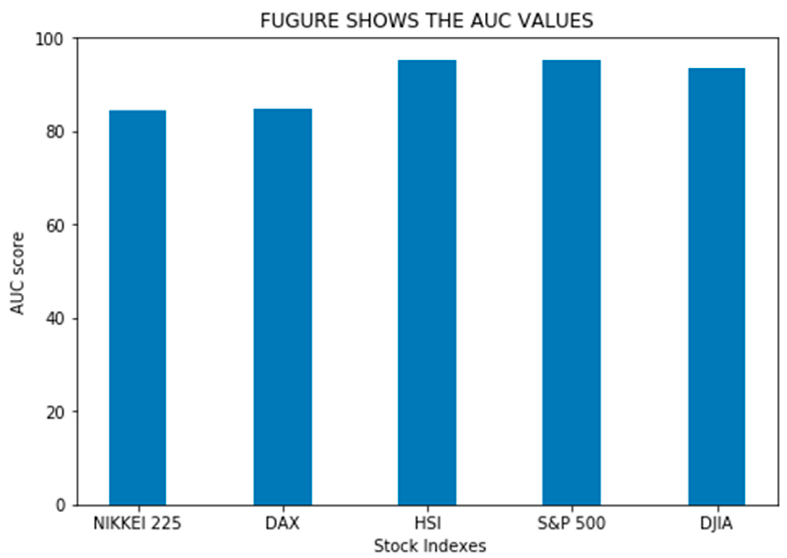
| INDEX | AUC SCORE |
|---|---|
| NIKKEI 225 | 84.41 |
| DAX | 84.71 |
| HSI | 95.26 |
| S&P 500 | 95.43 |
| DJIA | 93.36 |
| Name of the Index | Our Proposed Model (Meta-LightGBM) | WLSTM+Attentation |
|---|---|---|
| MAE | MAE | |
| S&P 500 | 0.0481 | 0.1935 |
| HSI | 0.0464 | 0.2453 |
| DJIA | 0.0672 | 0.1569 |
| Training Accuracy | Testing Accuracy | Difference | Dataset | |
|---|---|---|---|---|
| Meta-LightGBM | 94.73 | 94.68 | 0.05 | S&P-500 Index |
| Meta-LightGBM | 95.09 | 94.97 | 0.12 | HSI Index |
| Meta-LightGBM | 93.33 | 93.27 | 0.06 | DJIA Index |
| Meta-LightGBM | 85.10 | 85.00 | 0.10 | DAX Index |
| Meta-LightGBM | 88.60 | 88.38 | 0.22 | NIKKEI 225 Index |
Publisher’s Note: MDPI stays neutral with regard to jurisdictional claims in published maps and institutional affiliations. |
© 2021 by the authors. Licensee MDPI, Basel, Switzerland. This article is an open access article distributed under the terms and conditions of the Creative Commons Attribution (CC BY) license (https://creativecommons.org/licenses/by/4.0/).
Share and Cite
Padhi, D.K.; Padhy, N.; Bhoi, A.K.; Shafi, J.; Ijaz, M.F. A Fusion Framework for Forecasting Financial Market Direction Using Enhanced Ensemble Models and Technical Indicators. Mathematics 2021, 9, 2646. https://doi.org/10.3390/math9212646
Padhi DK, Padhy N, Bhoi AK, Shafi J, Ijaz MF. A Fusion Framework for Forecasting Financial Market Direction Using Enhanced Ensemble Models and Technical Indicators. Mathematics. 2021; 9(21):2646. https://doi.org/10.3390/math9212646
Chicago/Turabian StylePadhi, Dushmanta Kumar, Neelamadhab Padhy, Akash Kumar Bhoi, Jana Shafi, and Muhammad Fazal Ijaz. 2021. "A Fusion Framework for Forecasting Financial Market Direction Using Enhanced Ensemble Models and Technical Indicators" Mathematics 9, no. 21: 2646. https://doi.org/10.3390/math9212646
APA StylePadhi, D. K., Padhy, N., Bhoi, A. K., Shafi, J., & Ijaz, M. F. (2021). A Fusion Framework for Forecasting Financial Market Direction Using Enhanced Ensemble Models and Technical Indicators. Mathematics, 9(21), 2646. https://doi.org/10.3390/math9212646