1. Introduction
Keynes created the basic framework of modern macroeconomics, but he did not establish a direct logically consistent relationship between the optimal decision making of micro-individuals and aggregate economic behavior. The parameters controlling the structural equation in the econometric model based on Keynesianism have changed, causing its predictability and explanatory power to collapse. In Keynes’s model, the formation of expectations is placed in the field of psychology instead of economics. The policy analysis does not fully consider the impact of policy changes on people’s expectations; that is, the Lucas’ critique. With the gradual development of economics, based on micro and macroeconomic theories, a dynamic stochastic general equilibrium (DSGE) model that uses dynamic optimization methods to examine the decisions of various actors (households, manufacturers, etc.) has emerged. The DSGE model has obvious structural characteristics in terms of the model setting, derivation of behavior equations, determination of parameters, identification of shocks, dynamic characteristics of the model and expected formation mechanism, etc., so the model exhibits neoclassical economics in the long term. The explicit modeling framework can truly enable the model to be communicated and improved between developers and users, and the simulation and prediction results of the model can be understood and trusted. In recent years, an increasing number of literatures are making use of the dynamic stochastic general equilibrium (DSGE) model to study the impact of various factors on the macro-economy and monetary policy [
1,
2,
3,
4,
5,
6,
7,
8]. With the rapid development and popularization of electronic money, an online mode not only provides convenience for payments, but also imperceptibly changes people’s payment habits and consumption behavior. It also brings unprecedented challenges to traditional financial theory, especially the impact on monetary policy [
9]. At present, there is no unified definition of e-money in academia. A more authoritative one is the definition issued by the Basel Committee in 1998; that is, e-money refers to the “stored value” and is “paid” in the retail payment mechanism, through sales terminals, between different electronic devices and on open networks (such as the Internet), which is a prepayment mechanism. “Stored value” refers to the value stored in physical media (hardware or card media) that can be used for payment, such as smart cards and multi-function credit cards. A prepayment mechanism is a set of electronic data that exists in a particular piece of software or network that can be transmitted and used for payment [
10]. Although this definition was made 22 years ago, there have been many definitions of electronic money, which were still controversial. The definition issued by the Basel Committee in 1998 has been quoted by scholars and regarded as the most authoritative and representative definition of electronic money. Therefore, we also chose to use this definition. The electronic money studied in this paper was a kind of “secondary” currency, which was the electronic money replacing the traditional currency. However, it had a one-to-one correspondence with the legal tender issued by the central bank, which was not a decentralized digital currency (such as Bitcoin). Compared with traditional money, electronic money is fast, low-cost, easy to carry, easy to preserve, has a high security and allows for long-distance payment, so it is favored by people. During the special period of the COVID-19 pandemic, more people tend to “shop online” and use “non-contact” electronic payment methods to reduce going out and gathering, reduce the use of banknotes and coins and block the spread of the epidemic. In addition, in the context of current green finance and sustainable development, electronic money will also become a more environmentally friendly and reliable payment method in the future [
11].
Although many factors may affect monetary policy, under the conditions of electronic money circulation, electronic money mainly affects monetary policy by influencing three monetary actors—consumers, commercial banks and central banks—and the impact of electronic money is mainly manifested in those three aspects. First of all, for consumers, the characteristics of electronic money make their daily transactions safe and convenient, and customers do not need to go out. This allows for them to complete the transfer of funds through online media, shortening the delivery time of payment instructions, improving the efficiency of capital operation and greatly reducing the “sole cost”. Second, for commercial banks, under the condition of electronic money, commercial banks can be a fast, low-cost way of financing, with the central bank not having the duty of being an electronic money reserve, so it is not necessary to retain a large number of commercial banks for excess reserves, which not only reduces the cost of bank management and improves the service efficiency, but also expands the business flexibility. Of course, electronic money will also bring a greater uncertainty to the traditional business of commercial banks. For the central bank, e-money will have a certain impact on the money supply and demand, and will increase the endogenous nature of the money supply and demand, thus affecting the implementation effect of monetary policy, and therefore creating greater challenges for the central bank in adopting monetary policy to regulate the domestic economy.
It can be seen that the emergence and development of electronic money has a real impact on all aspects of the social economy. Macroeconomic variables are more or less affected, and the implementation and effectiveness of the central bank’s monetary policy is also more obvious. Therefore, this paper constructs a DSGE model based on electronic money shock to investigate the changes in macroeconomic variables under the impact of electronic money. This will more effectively analyze the impact of electronic money from the perspective of the micro subject. Therefore, the research of this paper has important theoretical value and practical significance for enriching and developing monetary policy theories and improving the effectiveness of monetary policy implementation. For this reason, a macro model was established under the condition of electronic money. The DSGE macro model was adopted and included three main bodies, which were commercial banks, central banks and households. Through the establishment of macro equations to explore the time and degree of changes required for each variable to reach equilibrium under the impact of electronic money, it can more effectively characterize the impact of electronic money on monetary policy through core variables, such as loans, savings and the interest rate, which also reflects, to a certain extent, the real operation of the economy.
The contribution of this paper is mainly in the following aspects: (1) The research perspective is novel. This paper studies the impact of electronic money on monetary policy from the perspective of consumers, commercial banks and central banks, and tries to study the effectiveness of monetary policy from a new perspective; (2) A DSGE model based on the behavior of three monetary subjects is constructed and simulated. This paper attempts to incorporate e-currency shocks into the main body behavior model and construct the DSGE model, estimate its parameters and solve the model, reveal the internal mechanism of the change in the main body behavior of money, focus on the change in the behavior of the central bank and evaluate the effectiveness of monetary policy; (3) The impact effects of electronic money under the two monetary policies are compared. The behavior of the central bank, namely monetary policy, is further divided into quantitative monetary policy and price monetary policy. By constructing their respective models and solving and simulating them, the differences between the two monetary policies and the effectiveness of the policies under the condition of electronic money are analyzed through impulse response results.
The following structure of this paper is arranged as follows: the second part is a literature review, which reviews and evaluates electronic money from three aspects: money supply, money demand and monetary policy effectiveness. The third part is the theoretical model, which aims to build the DSGE model based on the behavior of monetary agents. The fourth part is parameter calibration, the selection of research variables and the calculation of the value of the parameter calibration. The fifth part is the simulation and analysis of the policy effect. Through parameter estimation, model solution and numerical simulation, the internal mechanism and policy effect of the monetary subject behavior change are analyzed. The sixth part comprises conclusions and recommendations.
2. Literature Review
At present, there are four main aspects of relevant research: the influence of electronic money on money supply, money demand and the effectiveness of monetary policy and the possible impact of a new kind of e-money, digital currency, on monetary policy.
2.1. The Impact of Electronic Money on Money Supply
If the issuance of electronic money is directly included in the total amount of money, electronic money will increase the money multiplier, thus increasing money supply [
12,
13]. Although e-money will influence the total money supply through base money and the money multiplier, the central bank can reduce various impacts of e-money on the money supply through the adjustment of the interest rate level and reserve ratio [
14]. Moreover, due to the different influences of e-money issued by different money-issuing subjects on the money supply, it is also difficult for the central bank to supervise them [
15]. Empirical research in different countries shows that e-money will influence the stability of the money supply in the short term, whereas, in the long term, it has little effect on the money supply [
16,
17,
18]. Research in China shows that the emergence and development of electronic money not only changes the form of money, but also changes the supply structure of money, and has a significant impact on money liquidity. The substitution of electronic money for paper money in circulation not only enlarges the money supply under the supervision of the central bank, but also enlarges the money supply outside the supervision [
19]. Other studies have shown that electronic money in the form of a third-party payment also has a significant impact on the money supply [
20].
2.2. The Impact of Electronic Money on Money Demand
Mainly, the impact of electronic money on the money demand is mainly reflected in two aspects: one is the speed of money circulation, and the other is currency substitution.
From the perspective of monetary velocity, the influence of electronic money on monetary velocity is complex, and is not only rising or falling, but a combination of various situations [
21]. Electronic money can accelerate the velocity of money circulation by influencing the central bank’s monetary control or monetary policy transmission mechanism [
10,
22,
23]. Through an empirical test, it is found that the development of electronic money will lead to the trend of the currency circulation speed falling first and then rising [
24,
25,
26]. Electronic money will increase the substitution between financial assets and accelerate the speed of the currency circulation [
27]. However, there are also studies that show that e-money substitution mainly has a substitution acceleration and substitution transformation effect, which leads to a long-term downward trend in the overall speed of China’s currency circulation [
9]. Moreover, third-party payments promote the speed of narrow money circulation in the short run, but inhibit it in the long run, and have the opposite effect on the speed of broad money circulation [
28].
In terms of currency substitution, if electronic money replaces deposits, the demand for money will moderately decrease, but even if the substitution of electronic money for the central bank currency will benefit enterprises and households, cash and settlement services provided by central bank cannot be replaced by electronic money [
14,
29]. The Canadian study also found that, although the substitution of electronic money reduces the share of cash payments, the impact of this substitution will not be too strong in the short term [
30]. It takes many years for more efficient electronic payments to be widely used, and the fees that merchants (consumers) pay for using those services are increasing (decreasing) over time [
31]. In recent years, many scholars have studied the determinants of e-money adoption in more micro ways. Social factors, effort expectancy, ease of e-money, facilitation conditions and even the COVID-19 pandemic may affect people’s use of e-money [
32,
33,
34]. However, the research results of China are different from those of foreign scholars. The substitution of electronic money for a transactional demand is not complete. It almost completely replaces the investment demand and produces a higher level of substitution for the preventive demand [
35,
36,
37]. Of course, this may be due to the rapidly increasing development of electronic payment and electronic money in China in recent years.
2.3. The Impact of Electronic Money on Monetary Policy
The research on the influence of electronic money on the effectiveness of monetary policy mainly embodies two aspects: the transmission process of electronic money on monetary policy and the control ability of monetary policy.
From the perspective of the transmission process of monetary policy, starting with the influence of monetary demand, this paper studies the effect of electronic money on the monetary policy and transmission mechanism of the central bank. The research shows that monetary demand not only increases the use of electronic money, but also affects monetary policy [
10,
38,
39]. When studying the influence of e-money on the base currency, if we consider the two cases that the central bank has statutory reserve requirements and no statutory reserve requirements for e-money, the results show that, in both cases, e-money will affect the total amount of the base currency, and will then affect the effect of monetary policy [
40]. At the same time, although e-money will affect the balance sheet of the central bank, the central bank can use the existing monetary policy to adjust in order to offset this part of the impact [
41]. Moreover, with the development of the Internet and communication technology, the gap between the bank overnight lending rate and the target interest rate has narrowed, and the monetary policy operation is better [
42]. Its large-scale circulation reduces the transmission efficiency of monetary policy to different degrees, deepens the endogenous of the money supply and weakens the correlation between the money supply and the ultimate goal of monetary policy, thus reducing the effectiveness of monetary policy [
43,
44,
45]. Some studies show that electronic money has significantly improved the effectiveness of China’s monetary policy, but this improvement has both a lag effect and an immediate effect [
46]. Other studies show that the influence of electronic money on monetary policy is uncertain, which enhances the effectiveness of monetary policy from the output channel and weakens the effectiveness of monetary policy from the price channel [
47].
Based on the assumption of monetary policy control, electronic money has its own independent system and becomes a private currency, and the central bank has lost the ability to move large transactions, reducing the control ability of monetary policy, where the central bank can only become a symbolic “indicator” [
48]. However, there are different views on this. Electronic money can only replace a small share of the basic money issued by the central bank. In real life, people still have a great demand for cash from the central bank. The study of China finds that commercial banks can evade the restraint of the rediscount and deposit reserve by increasing e-money. At the same time, electronic money may make the central bank lack sufficient assets and liabilities to better carry out open market operations, thus greatly affecting the central bank’s ability to control monetary policy [
49,
50].
2.4. The Impact of Digital Currencies on Monetary Policy
As a new form of electronic money, digital currencies, which, in some situations, are called cryptocurrencies, also have some impact on monetary policy. Digital currencies can be issued in two ways: decentralized and centralized [
51]. Among them, most privately issued digital currencies, such as Bitcoin, belong to decentralized digital currencies, whereas central bank digital currencies (CBDCs) are centralized currencies issued by central banks, which are essentially different from each other. For the decentralized digital currencies, there is a consensus that they may not play the role of a traditional currency, which satisfies three basics functions of a currency: the means of value scale, circulation and storage [
52]. Some specific studies on Bitcoin have suggested that the replacement of Bitcoin for traditional currencies would destroy the existing payment system, thereby adversely affecting the monetary system and the real economy [
32]. In addition, decentralized digital currencies will bring risks to the effectiveness of monetary policy, financial stability and economic growth [
53,
54,
55,
56]. For the central bank digital currencies, which have a one-to-one correspondence with the legal tender, just like the traditional e-money, most scholars believe that issuing CBDCs will help to improve the effectiveness of monetary policy, and many have reached consensus in this regard [
57,
58,
59,
60,
61,
62]. However, some scholars have also raised concerns about central bank digital currencies, such as narrow banking, raising bank funding costs and reducing investment [
63,
64,
65,
66].
In summary, the existing relevant research has made breakthroughs in many aspects and has made many valuable achievements, which is also the important basis of this paper. Due to the emerging research field of electronic money and the rapid development of Internet finance, financial technology and electronic money in China in recent years, there has been a lot of relevant research on China. However, there are some shortages in existing research: first, regarding the research content, the existing research mainly discusses the electronic money impact on the money supply and money demand, starting from the various influence factors, such as the monetary base, money multiplier and currency substitution, putting forward relevant suggestions. In this paper, monetary policy and the macro system is included, and the influence of the economic operation mechanism is stated in detail, which may fill in the gaps in the knowledge of this stream of references in China. Second, regarding the research methods, the existing research focuses mostly on the electronic money factors affecting the money supply, whether they have a significant correlation and how to develop a more inclusive monetary policy, putting forward relevant suggestions; however, few articles go through the DSGE model to study the electronic money. This paper uses the DSGE model to illustrate how the economic subject behavior influences the effect of monetary policy. Third, regarding the research framework, most of the literature studied the influence of electronic money on monetary policy through theoretical analysis, and put forward relevant policy suggestions. However, there is no further analysis of the type of monetary policy through a clear decision formula (such as the Taylor rule), and few literatures put forward relevant suggestions in a targeted way. This paper tries to give more reasonable suggestions based on the model’s numerical results. In short, the research on the impact of electronic money on monetary policy is not systematic and in-depth enough, which creates a certain space for the research of this paper.
Due to space limitations, this article does not discuss the impact of digital currencies on monetary policy in depth. Besides, some parameter calibrations in this article refer to the existing literature without further empirical research. This may be a limitation of this article.
3. Model
As the mainstream economic analysis model in the fields of macro-economy, monetary policy and fiscal policy, the DSGE model starts from the perspective of the aggregate demand and supply of New Keynesianism and adopts the combination of theoretical modeling and stochastic simulation in order to effectively observe the dynamic change relationship among economic variables and accurately measure the expected trend. Based on the micro theory, the model considers the optimal behavior of each economic entity, including the representative maximization behavior of the household utility, the maximization behavior of the manufacturer profit and the decision-making behavior of the central bank. Each economic entity realizes the optimal decision under different constraints. The model has the advantages of an explicit modeling framework and is closely combined with a macro and micro analysis and with a long-term and short-term analysis organically, which is more comprehensive than the traditional method [
67]. Many central banks, financial departments, the International Monetary Fund and other institutions are also developing DSGE models with different complexities, which are widely used in financial market practices, such as central banks, commercial banks, the interest rate and foreign exchange rates [
68,
69,
70,
71,
72,
73,
74]. The DSGE models have developed rapidly since the global financial crisis in 2008, and one survey showed that 84 different DSGE models exist that have been developed by 58 institutions [
1]. Recently, the DSGE model was widely used in the field of monetary policy [
75,
76,
77,
78,
79]. Therefore, the DSGE model has become the mainstream research method in the field of economic research and policy analysis, and there will be a greater need for future DSGE policy models to adopt more recent findings in empirical literature.
This paper aims to study the impact effect of e-money on monetary policy and, specifically, to explore the impact of the behavior changes in main monetary subjects, such as households, commercial banks and the central bank, on monetary policy under the impact of e-money. This paper needed to objectively consider the close combination of the theoretical model and empirical simulation, the dynamic changes in macro and micro monetary entities and the effect of long-term and short-term monetary policy, and the demand for research methods is naturally consistent with the advantages of the DSGE model. Therefore, it is more appropriate to choose the DSGE model. Although SVAR, stochastic simulation and other traditional methods can also be chosen to study the problem mentioned in this paper, they have limitations; for example, the SVAR model can also identify many exogenous random shocks, but cannot carry out dynamic analysis and explain the problem of the intertemporal optimal decision. It also cannot achieve the general equilibrium of products, labor, capital and other markets. Therefore, the DSGE model selected in this paper should be the best.
In order to explore the impact of e-money on monetary policy, a universal DSGE model based on e-money was constructed, which can represent most countries. The modeling of this paper was divided into two parts: the first part was to analyze the impact of e-money on the behavior of the subject from the three perspectives of the residents, commercial banks and the central bank, forming a relatively systematic theoretical system. Then, the impact of e-money on consumption was reflected in the mathematical model of each subject, and the DSGE basic model, including the impact of e-money, was built and solved. The second was to include the restraining impact caused by the risk of e-money into the basic model, forming an extended model that included the promotion impact and the restraining impact of e-money.
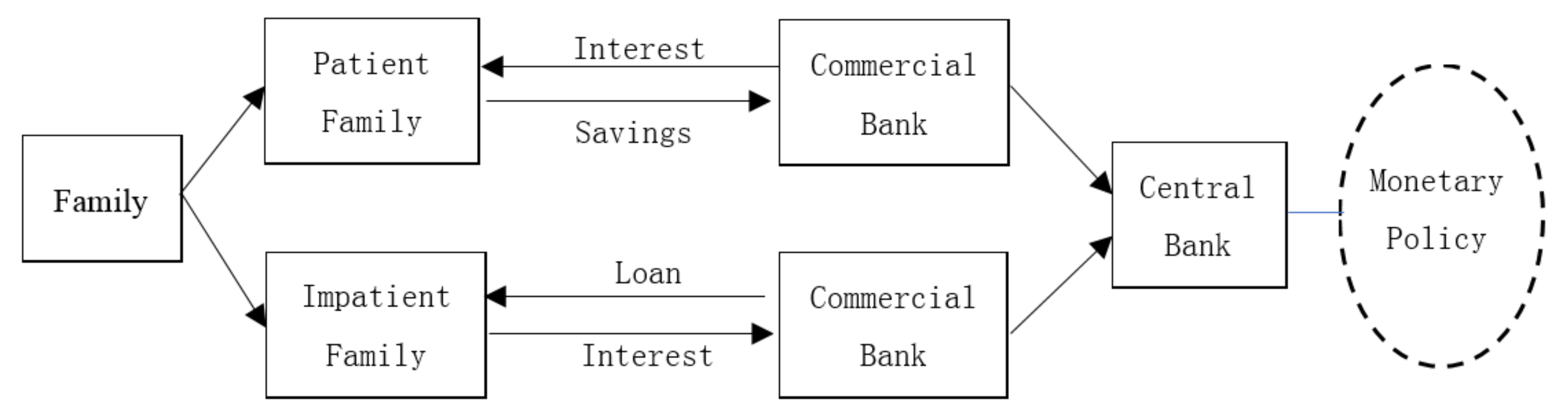
The DSGE model based on the new Keynes framework can effectively establish monetary policy rules and depict the optimal behavior of households, commercial banks and central banks, and reflect the operation dynamics of the real macroeconomic system. The DSGE model constructed in this paper includes three economic entities, namely, households, commercial banks and central banks. The behavioral relationship among economic entities is shown in
Figure 1. The core of the DSGE model established in this paper is from the perspective of money, and relevant variables (such as loans and savings) are directly related to money, which facilitates an in-depth discussion of the impact of electronic money on monetary policy.
3.1. Assumptions
Before modeling, several assumptions are proposed as follows:
3.1.1. There Are Two Kinds of Heterogeneous Families: Patient and Non-Patient
This assumption is made according to Kiyotaki and Moore [
80], who raised the issue of heterogeneous agents for the first time, which is an extensive application in the analyses in a DSGE model [
81,
82,
83,
84]. This assumption is in line with reality because the saving rate differs from each family, and can bring better explanatory power to the model.
3.1.2. The Commercial Bank Is in a Perfectly Competitive Market; Commercial Banks Absorb Deposits from Patient Families and Grant Loans to Non-Patient Families
This assumption is made referring to Liu Zhilin’s model set up in 2016 [
85]. The first half of the assumption can help us to determine the interest rate level, and the second half can help us derive the asset allocation of the two types of households.
3.1.3. The Central Bank Mainly Adopts Quantitative Monetary Policy and Price Monetary Policy
This assumption is made for the central bank to regulate and control the economy, which is in line with reality.
3.1.4. Market Clearing and Price Stickiness
These assumptions are the two important assumptions for the DSGE model [
86].
3.2. Family
According to
Section 3.1.1, patient households have a higher tendency to save, where saving brings a higher utility than consumption, and impatient households have a higher tendency to consume, where consumption brings a higher utility than savings. Here, we introduce electronic money to analyze the utility of two types of households. It is important to note that, since the global financial crisis in 2008, most western countries have implemented unconventional monetary policies (a negative or zero interest rate and quantitative easing), which have a significant impact on the savings utility of patient households, and even produce negative effects. Although there were many financial instruments to choose from, patient families can only choose bank deposits with a relatively low risk under the circumstances of uncertain economic growth, fierce financial market volatility and a high risk of financial market instruments. The implementation of unconventional monetary policy was not a normal choice, but a choice made in a special period (such as a financial crisis). We only considered the general situation when we analyzed the impact of electronic money on monetary policy. Since the later simulation was based on China’s data, it is more realistic to focus on bank deposits, which can also represent the situation of most countries.
Patient families try to maximize their utility function:
In the formula, is an intertemporal discount factor for patient families; , represents patient household consumption and savings in the t period, respectively; is the proportion of household consumption in the utility function; stands for the promotion coefficient of e-money to consumption. The existence of e-money greatly reduces transaction costs and improves transaction convenience, which will promote household consumption to a certain extent. Therefore, we will also express as the change in consumer preferences of e-money, and its impact will increase with the increase in e-money transaction penetration. Therefore, we assume that and that follows the autoregressive process. The equation represents the equation of model shock. Generally speaking, the impact from the macro level had certain inertia. Therefore, it was generally assumed that the model shock in the DSGE model was first-order autoregressive, and that the residual term was assumed to follow the autoregressive equation. In this equation, we studied the impact of the rapid development of electronic money on the residents’ decision-making equation, which further affected the behavior equation of commercial banks and central banks. Finally, according to the adjustment of various variables, the economy formed by the three main bodies reached a new equilibrium. Equation (1) represents the utility function of the patient family. In our model, compared with the non-patient family, the patient family was more likely to choose savings in order to meet the delayed consumption. Therefore, the utility of the patient family came from two parts: one was to improve the current consumption, and the other was to meet the savings for future consumption. In fact, for a patient family, the current savings increment, rather than the absolute amount of current savings, was the variable that best reflected the current utility. Therefore, this model adopted the index of the savings increment. The logarithm of consumption was used because it was easy to find the first-order optimal solution by processing the data without changing the increase and decrease in the function. Currently, most of the literature dealt with the variables by means of logarithm. We have added relevant explanations in the revised version.
Its budget constraints are:
In the formula,
represents the deposit rate of commercial banks in the t period, and
represents the rate of inflation in the t period. Equation (2) represents the budget constraint for those patient families. This model assumed that the source of funds in the current period was the amount of savings in the previous period multiplied by the rate of return on investment and then divided by the level of inflation, which was the sum of consumption and savings in the current period. In this equation, the denominator reflected the level of price. If inflation occurred, the denominator value was greater than 1, which can be used to eliminate the impact of inflation on the equation. It can be concluded that the first-order conditions for the optimal economic behavior of the patient family sector are:
In Formulas (3) and (4),
represents the multiplier for patient household borrowing constraints, instead of patient households trying to maximize the following utility functions:
In Formula (6), , is an intertemporal discount factor for impatient families; , represents the consumption of impatient households and loans in t period, respectively; is the proportion of household consumption in the utility function; represents the promotion coefficient of electronic money to consumption. Here, we include the loan variable in the utility function because impatient households have a higher propensity to consume, and they prefer to consume ahead of time in order to maximize their expectations, which is equivalent to a short-term loan.
Its budget constraints are:
In Formula (7), represents the interest rate of commercial bank loans in the t period.
It can be concluded that the first order condition of the optimal economic behavior of the impatient family is:
In Formulas (8) and (9), represents the multiplier for impatient household borrowing constraints.
In addition, both patient families and non-patient families are facing constraints on the total consumption of consumer goods.
Equation (11) shows that the current consumption expenditure C1 of the patient family plus the consumption expenditure C2 of the impatient family must be less than or equal to the total output Y of the economy. It was assumed that there were only two groups in the economy. One was the patient family and the other was the non-patient family. Therefore, in terms of supply and demand, these two were balanced. When seeking the optimal solution, the equal sign was adopted to solve in this paper.
3.3. Commercial Bank
The interest rate channels, credit channels, financial asset price channels, exchange rate channels and balance sheet channels are the main channels that affect the transmission of monetary policy; however, as analyzed above, since the influence of electronic money on the transmission of monetary policy is mainly manifested in the transmission of the interest rate, the impact of other factors on monetary policy was not considered in this paper. According to Assumption 3.1.2, families’ assets mainly come from deposits
and capital
, while the source of profits is obtained by lending assets
. Therefore, the optimal behavior decision-making problem of commercial banks under capital constraints can be expressed as follows:
In Formula (12),
represents the deposit interest rate of commercial banks in the t period;
represents the interest rate of commercial bank loans in the
t period;
is the actual capital rent rate. The constraints are as follows:
Then, the first-order conditions for the optimal behavior of commercial banks are as follows:
In Formula (14), is the capital adequacy ratio of commercial banks; that is,
3.4. Central Bank
In quantitative monetary policy, referring to Liu ’s model [
85], an inflation expectation is introduced into the nominal monetary growth rate; that is,
, and using the money supply as the proxy variable of quantitative monetary policy, the following expression can be obtained:
In Formula (15), is the impact sustainability parameter of money supply, is the weight coefficient of the inflation expectation and is the weight coefficient of the output gap.
Regarding interest rate as the proxy variable of price-based monetary policy, it is assumed that the central bank adopts the generalized Taylor rule:
In Formula (16), is the impact persistence parameter of the interest rate, is the weight coefficient of the inflation expectation and is the weight coefficient of the output gap.
3.5. Model Steady State
After solving the behavioral equation of the family, commercial bank and central bank, and based on Assumption 3.1.4, we can solve the steady value of model variables.
An asterisk represents the steady-state value of the variable. After the establishment of the model, we calculated the steady-state value (equilibrium value) of each variable by a linearization method. This steady-state value was a definite value, not a variable. In the impulse response, we can obtain the time and process for each variable in order to reach the steady-state value through the Dynare of Matlab.
Therefore, the DSGE model constructed in this paper consists of Formulas (1)–(16). Endogenous variables include {, , , , , , , , , }, parameters include{, , , , , , , , , , , , , } and exogenous impact variables are {}.
3.6. Model Extension Considering the Risk of Electronic Money
According to the above-mentioned basic model, in order to further analyze the impact effect of e-money on monetary policy, the impact of the e-money risk was included in the basic model and an extended model was formed that included the e-money promoting impact and restraining impact. The steady-state values of the model variables were solved by combining the behavior equations of the family, commercial bank and central bank.
Since its development, electronic money has brought a lot of convenience to micro subjects by virtue of its convenience, universality and other characteristics; however, behind the irrational exuberance is the shadow of crisis. Due to the imperfect supervision of the electronic money business, its business has not implemented access management, and it is easy to form a situation where the default revenue exceeds the default cost. Errors, malfeasance, fraud and other results or behaviors caused by reasons other than the issuing entity or customers of electronic money will also force the issuing entity to take credit risk.
Behind the infringement of investors is the fact that the illegal elements make use of the inadequate supervision of the electronic money market, but are favored by the private families. By publicizing Internet products, such as “high income” and “rigid payment”, they win the public’s radical mentality and thus achieve the purpose of illegal fund-raising. The occurrence of these thunderstorms will slowly erode the public’s desire to use electronic money products, and will reduce the public’s attitude towards new products. According to a survey of 536 college students from 134 colleges and universities conducted by the China University Media Union in 2018, 57.46% of the students surveyed accepted low-threshold new concepts and were cautious, 28.54% of the students surveyed maintained a vigilant attitude towards low-threshold new concepts and seldom used them and 5.97 percent were open to and embraced these kind of concepts [
87]. This cautious attitude will also weaken the impact of e-money to a certain extent, which also provides theoretical support for us to incorporate the impact of e-money risk into the behavior framework of the monetary subject in the model.
3.6.1. Family Model Extension
The risk of e-money will make residents discount under the effect of the original consumption promotion. Therefore, in this paper, we add the inhibitory factors to the consumption under the effect of the original model of e-money, and obtain the revised family behavior model.
Patient families try to maximize their utility function:
In Formula (26)
indicates that the risk of e-money is a deterrent to household consumption. Similarly, we assume that
follows an autoregressive process. The first-order condition for the optimal economic behavior of the patient family sector can be obtained by the simultaneous Formula (2):
Formulas (27) and (28) represent multipliers of patient household lending constraints.
Non-patient families try to maximize the following utility functions:
The first-order condition of the optimal economic behavior of the impatient household sector can be obtained from the simultaneous Equation (7). The first-order condition of the optimal economic behavior of the impatient household sector is as follows:
In Formulas (31) and (32), indicates multipliers of impatient household lending constraints.
3.6.2. Steady State of the Model
After solving the behavioral equation of the family, commercial bank and central bank, we can solve the steady value of model variables.
Therefore, the DSGE model constructed and expanded in this paper includes Formulas (2), (7), (11)–(16), (26), (27)–(30) and (31)–(33). Endogenous variables include {, , , , , , , , , }, parameters include {, , , , , , , , , , , , , , } and exogenous impact variables are {, }.
4. Variables and Parameters
Recently, due to the rapid development and popularization of e-money in China, the impact of e-money on monetary policy is also growing. In addition, as the development of e-money in different countries is different, there are various circulation modes, and the relevant data are difficult to obtain. Therefore, in view of the availability of data, this paper only chose China’s data for simulation. However, the simulation results and policy implications also have great reference value for other countries.
4.1. Variables Selection
In this paper, the selected variables include total bank card transactions, P2P online loan transactions, household savings and consumption and urban savings and consumption. The time range of the total bank card transaction data is from March 2009 to September 2018. The total bank card transaction data are quarterly data with a total of 39 pieces of data, while the P2P online loan transaction volume uses monthly data with a total of 57 pieces of data. The time range of the P2P network loan transaction data is from March 2014 to November 2018. In the processing of the two parts of the data, the seasonal adjustment method and H-P filtering method are used to eliminate the influence of trend items of variables and to make them conform to the model for the steady state. The requirements are that the remaining data time range is from 1998 to 2017 annual data and that data processing only needs to use the H-P filtering method adjustment. All data are from Wind Financial Database (Wind) [
88].
4.1.1. Electronic Money Promotes Shocks
In this paper, we assume that the impact of e-money on consumption follows a first-order autoregressive process, and that the coefficient A in the regression equation actually measures the growth rate of the steady impact of e-money. In order to quantify the growth rate of shocks, we approximate the calculation with the transaction amount data of bank cards. By putting the growth rate sequence of the transaction amount into the first-order autoregressive model, we can obtain the growth rate of shocks and the distribution of residual terms. The estimation formula is
, where the original data are normalized after removing trend terms. Finally, the persistence parameter A of the promoting effect is obtained by first-order autoregression.
In Formula (44), if the regression coefficient is 0.891, it indicates that e-money has a significant role in promoting residents’ consumption. If the coefficient of determination is 0.998, it indicates that the goodness of fit is very high and that the regression effect is very good. The residual term is a normal random distribution with a mean value of −0.005 and a standard deviation of 0.013.
4.1.2. Electronic Money Suppresses Shocks
In consideration of the impact of electronic money risk factors on consumer consumption, we also assume that the inhibition impact of electronic money on consumption follows the first order autoregression process, and that the coefficient B in the regression equation is the growth rate of steady impact. In the process of parameter estimation, we select the p2p lending market data with a relatively concentrated e-currency risk. As can be seen from the sample data, although the transaction volume in the p2p online loan market rose slowly from 2015 to 2017, the year-on-year growth rate of the transaction volume in the online loan market has been steadily decreasing since 2015. Therefore, we first reduce the year-on-year growth rate of monthly P2P loan transaction volume by 2%, and then put it into the first-order autoregressive model to obtain the impact growth rate and the distribution of residual terms, where the estimation formula for
. After the trend term is removed, the original data are normalized, and the persistence parameter B of the inhibitory effect is finally obtained through first-order autoregression.
In Formula (45), if the regression coefficient is 0.851, it indicates that the e-money risk has a significant impact on the residents’ consumption. If the coefficient of determination is 0.986, it indicates that the goodness of fit is very high and that the regression effect is very good. The residual term is a normal random distribution with a mean value of 0.008 and a standard deviation of 0.018.
4.1.3. The Proportion of Consumption to Utility ,
In estimating the parameters of the consumption-to-utility function, we first approximate urban residents as patient families and rural residents as impatient families. Secondly, the selected annual data of savings and consumption of urban and rural residents are processed with the de-trend item. Then, regarding the processed data, the proportion of annual consumption to savings and consumption is calculated, and the coefficient of consumption item in utility function is obtained by taking the average value. Finally, it is estimated that the proportion of urban residents (patient families) and rural residents (non-patient families) is 0.337 and 0.455, respectively, where and .
4.2. Calibration of Parameters
The DSGE parameter calibration in this paper is mainly realized by referring to existing literature and parameter estimation. Referring to Liu’s estimation [
85], the subjective discount factor of the two families is 0.98 and 0.96 for
and
, respectively. The sustainability parameter of quantitative monetary policy
shocks is 0.6 according to Ma’s estimation [
89]. The sustainability parameters of the type of monetary policy on prices
is set to obey averages of 0.5 beta distribution. The weight coefficients of inflation expectation
in quantitative monetary policy, output gap in quantitative monetary policy, inflation expectation in price monetary policy
and output gap in price monetary
policy
are set to 0.04, 0.06, 0.08 and 0.06, respectively, according to Liu et al. [
90]. Parameter calibration values are shown in
Table 1.
5. Numerical Simulation
We numerically simulate the basic model and the extended model to analyze the impact of e-money on monetary policy. Under the framework of price-based monetary policy, this paper compared the impact of e-money on promoting and restraining the impact of e-money, and explained the difference between the response of e-money to the impact of savings, loans, output and the interest rate, and further analyzed the impact of e-money on monetary policy from two aspects.
5.1. Impulse Response Analysis of Basic Model
Through the use of the Matlab Dynare toolbox for analysis, we can obtain the impulse response graph of various macroeconomic variables of the e-currency impact introduced in this paper, so as to more intuitively understand the impact degree of the e-currency on various economic variables. The abscissa of the impulse graph is the quarterly period and the ordinate is the deviation of the variable from its steady-state value level. Since the unit of the impulse graph is the percentage, in order to facilitate analysis and understanding, the following analysis takes 0.01 as the basic unit.
5.1.1. The Response of Major Variables to the E-Currency Promotion Shock under the Price Monetary Policy
Figure 2 shows the response of domestic savings, loans, output and the interest rate to the impact of an increase of one percentage point in e-money transactions.
When the savings were hit, the deviation from the steady-state value reached its peak in phase 2, dropping by 18 units, and then slowly recovered, returning to the steady-state value after phase 35. When the loan was impacted, the deviation range increased, and then slowly fell back to the equilibrium state. It deviated from the steady-state value by 10 units in the third phase, and returned to the steady-state value level after the 40th phase. When the output was impacted, it deviated from the steady-state value by 23 units in phase 1, and then returned to the steady-state value level after phase 35. When the interest rate was hit, the deviation from the steady-state value reached its peak in the first period, rising by two units, falling rapidly in the second and sixth period, decreasing by 0.2 units from the steady-state value in the sixth period and then returning to the steady-state level after the 27th period. Through impulse response analysis, we can see that the impact of e-money shock on savings is larger and lasts a shorter amount of time than that of loans, and the total domestic output can quickly recover to the steady-state level when receiving the impact of e-money. It is worth noting that the interest rate rises briefly when it is hit by electronic money, then falls rapidly below the steady-state level and slowly returns to the steady-state value.
- (1)
Asymmetric effects of electronic money on savings and loans
In the impulse response results, we can see that the impact of e-money on savings and loans has an asymmetric effect. The impact on savings is greater and lasts for a shorter amount of time than that of loans. As a result of its convenience and convenience, electronic money reduces the time cost and capital cost of people’s transactions to a certain extent, and enhances the consumption desire of residents. The stimulation of e-money to consumption is mainly embodied in two aspects: one is to reduce more savings by promoting patient families, and the other is to increase their consumption level by stimulating non-patient families to increase more loans.
Behind this phenomenon, it reveals from another angle that saving is a sensitive variable for Chinese families at this stage. As is well-known, since the reform and opening up, China’s saving rate has been high, ranking at the forefront of the world. There are many drawbacks of excessive savings, which may cause potential economic growth to be difficult to manifest, and also can easily lead to overcapacity. The empirical results of this paper show that, in the era of convenient transaction and greatly improved transaction technology, patient families are easy to change in behavior; that is, families with high savings are more likely to reduce savings to improve their consumption level, and e-money has a more significant effect on the level of consumption of residents.
The asymmetric effect of savings and loans will also bring great challenges to the operation of commercial banks. As is well-known, household savings are the debt of banks, and household loans are the assets of banks. In the process of the transformation of Chinese commercial banks, the proportion of traditional credit business declines, and that of intermediary business rises. However, in a short period of time, under the background of no assets with higher returns, traditional credit is still the main profit source of commercial banks. The asymmetric effect of savings and loans will profoundly affect the assets and liabilities management of commercial banks. It will also have a great impact on the existing liquidity supervision system. The contradictions between the gap between assets and liabilities and the structure, term matching, etc., will also be highlighted under the effect of electronic money. How, then, can commercial banks formulate corresponding measures to deal with them? Challenges and how to take advantage of e-money opportunities under the premise of effective risk control will be the problems that many financial institutions have to face.
- (2)
The Impact of Electronic Money Shock on Interest Rate
In this paper, the empirical study found that the influence of electronic money on the interest rate has a reverse effect: at the beginning of the impact, the interest rate will rise to a larger extent, and will then fall back to equilibrium level. This is different from the existing research that electronic money will enlarge the money supply by reducing the reserve, thus reducing the interest rate. According to the conclusion of the existing literature, the existence of electronic money will magnify the money multiplier and have a positive impact on the money supply. At the same time, electronic money has an impact on the velocity of money circulation, and promotes the emergence of money substitution. The interest rate is the most direct determinant of the currency demand and currency supply, and, combined with the empirical conclusion, we can find that, in the process of the influence of electronic money on the interest rate, the sharp rise in the short-term interest rate appears because of the influence of the money demand holding the dominant position; more electronic money reduces the money velocity, promotes the currency substitution and then increases the cost of loanable funds. However, in the medium and long term, the influence of the money supply starts to appear, and electronic money accelerates the velocity of money circulation. Finally, the interest rate will show a large decline and return to the level of the equilibrium interest rate.
The reversal of the interest rate also means that the two variables of the money supply and demand have a different sensitivity to electronic money. When shock from electronic money occurs, the money demand will change rapidly in response, and then the money supply will gradually come into play until the market is cleared. This kind of lag phenomenon causes the interest rate volatility of the market in a short period of time, induces the micro main body to make the wrong decision and even affects the normal operation of the economic system. In this regard, the central bank can make corresponding adjustments to smooth out fluctuations, such as implementing a certain amount of short-term reverse repos when hit, in order to make up for the short-term liquidity shortage.
5.1.2. Response of Major Variables to E-Money Promoting Shocks under Two Kinds of Monetary Policies
Under the two kinds of monetary policies, the difference in e-money impact is mainly reflected in the two variables of the interest rate and nominal money growth rate. As can be seen from
Figure 3, when the interest rate was impacted, it deviated from the steady-state value to the highest point in the first period, rising by two units, and rapidly declined in the second to sixth periods. By the sixth period, it dropped by 0.2 units compared with the steady-state value, and then recovered to the steady-state level after approximately the 27th period. When the nominal money growth rate was impacted, it deviated from the steady state value at the highest level in the first period, falling by 23 units. It rose rapidly from the second to the seventh period, rising by five units compared with the steady-state value by the seventh period, and then returned to the steady-state level approximately 37 periods later. This shows that, in the face of the impact of electronic monetary policy, the two monetary policies greatly differ regarding the impact of electronic money. The impact of electronic money on price monetary policy is smaller than that of quantitative monetary policy, and its duration is shorter.
5.1.3. Price Policy Is Better than Quantity Policy
From the effect of the quantitative monetary policy and price monetary policy on the impact of electronic money within the sample range, the price monetary policy with interest rate as the core variable is less affected and has a shorter duration than the quantitative monetary policy with money supply as the core. On the one hand, this result indicates that, under the impact of electronic money, the regulation effect of price monetary policy is better than that of quantitative monetary policy; on the other hand, it indicates that electronic money will have a great impact on the money supply as the intermediary target of monetary policy. From the perspective of measurability, the enhancement of the substitution between financial assets will greatly increase the difficulty of the monetary quantity calculation, because electronic money blurs the division of the monetary hierarchy. In terms of the control ability, the emergence of electronic money will change the monetary velocity, reserve requirement and other variables, and affect the control ability of the central bank for monetary policy. In terms of correlation, the emergence of electronic money weakens the correlation between the money supply and the ultimate goal.
Under the background of the completion of interest rate marketization in China, China should still vigorously explore the effect of price-based monetary policy at this stage, giving full play to the price discovery function of price-based monetary policy, the transmission channels of monetary policy, the independent pricing ability of commercial banks and so on. It is necessary to improve the overall management level and operational efficiency of the financial industry, promote its financial innovation, and then establish and improve the price-based monetary policy regulation and transmission mechanism with the interest rate of the central bank as the core and the market-oriented interest rate as the intermediate target of monetary policy, so as to enhance the independence of China’s monetary policy.
5.2. Impulse Response Analysis of Extended Model
Through using the Dynare toolbox of MATLAB to analyze, we can obtain the impulse response graph of each macroeconomic variable to the impact of e-money introduced in this paper, so that we can understand the impact degree of e-money on economic variables more intuitively. The abscissa of the impulse graph is a quarter period, and the ordinate of the impulse graph is the deviation of the variable relative to its steady-state value.
5.2.1. Impulse Response of Risk Suppression Shocks
- (1)
The Response of Main Variables to the Shock Suppression of Electronic Money under Price-based Monetary Policy
Figure 4 shows the response of domestic savings, loans, output and the interest rate to the impact of e-currency risk growth of one percentage point. When savings are impacted, the deviation from the steady-state value increases in the short term. In the second phase, the deviation from the steady-state value reaches its peak, rising by eight units, and then slowly declines, returning to the steady-state value after the 30th phase. When the loan is impacted, the deviation from the steady-state value in the third period is the largest, reaching six units, and it returns to the steady-state value level after the 30th period. When the output is impacted, it deviates from the steady-state value by 12 units in phase 1 and then returns to the steady-state value after phase 25. When the interest rate is restrained, the impact will also appear, which is similar to the shock reversal effect of the interest rate in the first period of the peak, which deviates from the value of the steady-state, drops by a unit, and then, in the second stage of slow recovery, compared to the steady-state value in the sixth period, rises by 0.1 units, and then slows down to approximately 25, falling back to a steady-state level.
From the analysis of the impulse response, we can see that the direction of the restraining impulse is basically the same as that of the promoting impulse, but the time to recover to the equilibrium is shortened. In addition, we find that the two variables of savings and loans will deviate from the steady state at the initial stage of the shock of the suppression of electronic money, and will then gradually return to the steady-state level, which has a greater impact on savings than the loan variable.
- (2)
Response of Major Variables to the Shock Suppression of Electronic Money under Two Kinds of Monetary Policies
Similar to the impact of e-money promotion, the difference in e-money impact under two kinds of monetary policies mainly reflects two variables: the interest rate and nominal money growth rate. As can be seen from
Figure 5, when the interest rate is shocked, the first period deviates from the steady-state value to the highest point, drops by one unit, slowly recovers in the second period, rises by 0.1 units compared with the steady-state value in the sixth period, and then slowly falls back to the steady-state level after approximately the 25th period. When the growth rate of nominal money is shocked, it deviates from the steady value in the first period and rises by nine units, drops rapidly between the second and the sixth periods, drops by two units compared with the steady-state value in the sixth period, and then rises slowly to the steady-state level after approximately the 25th period. This result also shows that the impact degree of the two kinds of monetary policies is quite different in the face of the impact of e-monetary policy. Price-based monetary policy with the interest rate as the core variable is less affected than quantitative monetary policy with the money supply as the core variable. Similarly, compared with the impact of e-money, the time for the two variables to return to the steady-state level is shorter.
- (3)
Effect analysis of risk suppression shock
From the above analysis, we can conclude that the effect of risk suppression shock and the effect of promoting shock are mainly different in the length of time for restoring equilibrium, where all variables under the impact of time are varying degrees of shortened. This means that the time required for dynamic adjustment of the model is short under the risk suppression shock. From the perspective of family behavior, the shortening of action time indicates that families show a strong sensitivity to risks and a fast attitude to adapt to the expectation of risks. After being shock from the risk, families will adjust their adaptability expectations more quickly. Therefore, the time required to reach equilibrium is shorter than that under the effect of promoting shock.
- (4)
Irrational deviation effect
In addition, through the impulse response, we can see that, under the impact of risk suppression, both savings and loans will deviate from the steady state in a short period of time, which is similar to the results obtained under the impact of e-money promotion, which means that e-money, whether promoting or as risk factors, will increase in a short period of time when the impact occurs. Families show a certain irrational state. Under the impact of the promotion of e-money, the family will have an irrational preference for this new tool in a short time (irrational preference means that the family’s preference for e-money will be higher than its own behavior decision), and the family’s investment behavior will become very radical. When the risk of e-money breaks out, the family will have a certain degree of irrational aversion (irrational aversion means that the family will have a higher degree of aversion to e-money than the risk aversion determined by its own behavior), and the family’s investment behavior will become very cautious. When families revise their behavior, the irrational factors gradually disappear, and then the behavior of saving and lending will gradually return to the equilibrium level.
5.2.2. Comparative Analysis of Promotion Shocks under Two Models
- (1)
The Response of Major Variables to the Impact of Electronic Money Promotion under Price-based Monetary Policy
Figure 6 shows the impulse response comparison of the main variables in the basic model and the extended model of e-money-driven shocks under price and monetary policy. Through
Figure 6, we can find that the volatility of the main variables increases in varying degrees after the risk factors are included. In the basic model, when shocked by the promotion of electronic money, savings in the first period decreased by 17 units compared with the steady value, and the second period deviated the most, reaching 18 units. Loans in the first period deviated 10 units from the steady value, the output in the first period deviated 23 units from the steady value and the interest rate rose by 1.3 units in the first period compared with the steady value. In the extended model with risk factors, when shocked by the promotion of electronic money, savings decreased by 14 units compared with the steady value in the first period, loans deviated from the steady value in the first period by five units, the output deviated from the steady value by 19 units in the first period and the interest rate increased by one unit compared with the steady value in the first period.
- (2)
Response of Major Variables to the Shock Suppression of Electronic Money under Two Kinds of Monetary Policies
Figure 7 shows the comparison of impulse response results between price-based monetary policy and quantitative monetary policy under the impact of e-money. From
Figure 7, we can find that the volatility of both policies has increased after the risk factors are included. In the basic model, when shocked by the promotion of electronic money, the interest rate rises by 1.3 units compared with the steady value in the first period, and the growth rate of nominal money decreases by 23 units compared with the steady value in the first period. In the extended model with risk factors, when shocked by the promotion of electronic money, the interest rate rises by one unit compared with the steady value in the first period, and the growth rate of nominal money decreases by 20 units compared with the steady value in the first period.
- (3)
Impulse response analysis
From the impulse response results, we can see that, regarding both quantitative and price monetary policies, in the model with risk factors, the volatility of each variable is smaller than that of the model without risk factors at the initial stage of the impact of e-money promotion, and it slowly receives over time. The process of convergence coincides with the conclusion that the promotion of e-money will be weakened after considering the risk factors.
In the data selection, we choose bank card data to represent the promotion impact and p2p network loan data to represent the risk impact. More broadly, the bank card market can represent a kind of electronic money market with an extremely stable credit degree and strong risk management ability, which can be called a strong credit market. However, the p2p online loan market can represent a kind of electronic money market with a high risk and easy credit decline, which can be called a weak credit market. In the context of the coexistence of the two markets, the impact of risks will bring a sharp contraction of the weak credit market, and investors will reduce the asset allocation to the strong credit market in the case of risk aversion. The two seemingly independent markets have a consistent co-movement, so, under the risk factors, the promotion effect of electronic money will be reduced.
Based on the empirical results of the extended model, we can describe the changes in investors’ behavior after considering risk factors. With the advent of risk shocks, investors will have an irrational aversion to the weak credit market in the short term because of risk events. Irrational aversion means that investors have a higher risk aversion to assets in a weak credit market than their own risk preference level. At the same time, due to this impact, investors are cautious about the e-money market, which also reduces the asset allocation in the strong reputation market. After that, investors begin to adjust their expectations of risk, and irrational aversion gradually disappears. Investors will gradually restore the allocation of strong and weak reputation markets. The whole allocation process will become rapid because investors are sensitive to risk. Finally, irrational aversion disappears. Investors will allocate their risk aversion level to both markets. Weak and strong reputation markets will return to equilibrium level, and all variables will remain stable.
6. Results and Implementation
The impact of e-money on savings and loans is asymmetric, whereas the impact on households is irrational. Under the impact of e-money, savings and loans show different degrees of impact, and the impact of savings is larger than that of loans, but the duration is shorter. This phenomenon shows that e-money has a significant effect on reducing savings and promoting consumer consumption. In the extended model, we find that savings and loans increase the deviation from the steady state in a short period of time regardless of the risk factors. This means that, in the early stage of the development of electronic money, families will show a certain degree of irrational preference, and, within a short time after the emergence of electronic money risk, families’ risk aversion will rise sharply, and families will show a certain degree of irrational aversion at this time. At the same time, the time for all variables to recover to the equilibrium under risk suppression shock decreases to different degrees, which means that the dynamic adjustment of the model under risk suppression shock takes less time due to investors’ strong sensitivity to risk.
The influence of electronic money on the interest rate has the reverse effect. The inverse effect of e-money on interest rate is that, at the beginning of the shock, there will be a large increase in the interest rate for a short time, which will then slowly fall back to the equilibrium level. The reason is that the money demand and money supply will show different hysteresis after being hit. At the initial shock, the change in interest rate is mainly guided by the money demand, so there will be a large increase. Then money supply factors come into play gradually, and the interest rate falls back to the equilibrium level. To some extent, the “inverse adjustment” of the interest rate increases the operating difficulty of micro subjects and affects the effectiveness of monetary policy.
Price-based monetary policy has strong anti-interference. Under the condition of electronic money, price monetary policy has stronger anti-interference than quantity monetary policy, which also means that the traditional system of taking the money supply as the intermediary target of monetary policy has been challenged. This is mainly due to the increase in the endogenous money supply under the influence of electronic money, and the weakening of the testability, controllability and relevance of the intermediate target of monetary policy.
E-money has the effect of risk restraint and shocks. There are two main effects of risk suppression shocks of electronic money. One is that some variables will deviate more because of investors’ irrational aversion for a short time after the shocks, and because investors are more sensitive to risk, the time to return to equilibrium will be shortened. Secondly, the risk restraint impact of e-money will reduce the promotion effect of e-money and bring greater uncertainty.
7. Recommendation and Discussion
The central bank should interfere with the effect of e-money on the interest rate in time: on the one hand, it should remain concerned about the impact of electronic money. It is important to monitor economic variables, prepare for policy intervention in advance, determine the layout of monetary policy tools, and ensure that the time cycle and scale of policy tools are consistent. On the other hand, the central bank should attach importance to the forecast guidance of micro-subjects, which will make the market produce irrational expectations. Therefore, we should provide behavioral norms and guidance to strengthen the ability to identify the micro-subject of monetary policy. In order to avoid the unreasonable fluctuation of short-term interest rate of individual enterprises, misleading decision-making, and then affect the normal operation of the economic system.
The central bank should re-examine the monetary policy objectives under the conditions of electronic money, and vigorously explore the effects of price type monetary policy, giving full play to the price discovery function of price type monetary policy. It can be seen from the empirical results that the price monetary policy has a stronger shock tolerance. In the future implementation of monetary policy, China should continue to promote price-based monetary policy and vigorously develop price-based monetary policy tools, while quantitative monetary policy should gradually be relegated to the auxiliary function. At the same time, the monetary policy decision-making mechanism should be clear, the role of each monetary policy tool should be clearly differentiated, the efficiency of the interest rate transmission mechanism of the banking system should be improved and the role of the price monetary policy tool should be maximized.
The household sector must take a cautious attitude towards electronic money and guard against the risks it may bring. Commercial banks must also carry out a good job in responding to the impact of electronic money on the banking business. Regulators should impose the risk management of electronic money. In terms of risk prevention, financial regulators can assist in establishing a fund depository mechanism and enforcing information disclosure requirements. In terms of behavior guidance, financial regulators should focus on guiding investors’ expectations of risks after they are impacted by risk events. In terms of risk control, after the occurrence of risk shock, financial regulators should always monitor the phenomenon of the prosperity of a strong credit market and control the possible irrational exuberance.
Though this article does not spend much time discussing it, as a new form of electronic money, the central bank’s digital currency is gradually becoming the mainstream currency form, and central banks of various countries have recently attached great importance to the research of CBDC. CBDC’s impact on monetary policy cannot be ignored. The traditional type of e-money and CBDC share some common features, such as convenience, a low cost and liquidity, while CBDC has its own advantages, such as stability, universality, programmability and security. Therefore, their impact on monetary policy will be different. An in-depth study of the impact of CBDC on monetary policy has important theoretical and practical significance for the central bank to regulate the number of digital currencies issued, flexibly use and innovate monetary policy tools, dredge the transmission channel of monetary policy and then improve the effectiveness of monetary policy. The methodology of this article is also applicable to research on CBDCs, which are also worthy of reference for another future research.


